Journal of Mathematical Finance
Vol.05 No.02(2015), Article ID:55152,24 pages
10.4236/jmf.2015.52009
On Two Transform Methods for the Valuation of Contingent Claims
Chuma Raphael Nwozo1, Sunday Emmanuel Fadugba2
1Department of Mathematics, University of Ibadan, Ibadan, Nigeria
2Department of Mathematical Sciences, Ekiti State University, Ado Ekiti, Nigeria
Email: crnwozo@yahoo.com, drcrnwozo@gmail.com, emmasfad2006@yahoo.com, emmasfad@gmail.com
Copyright © 2015 by authors and Scientific Research Publishing Inc.
This work is licensed under the Creative Commons Attribution International License (CC BY).
http://creativecommons.org/licenses/by/4.0/


Received 3 March 2015; accepted 27 March 2015; published 30 March 2015
ABSTRACT
This paper presents two transform methods for pricing contingent claims namely the fast Fourier transform method and the fast Hilbert transform method. The fast Fourier transform method utilizes the characteristic function of the underlying instrument’s price process. The fast Hilbert transform method is obtained by multiplying a square integrable function f by an indicator function associated with the barrier feature in the real domain. This is also obtained by taking the Hilbert transform in the Fourier domain. We derived closed-form solutions for European call options in a double exponential jump-diffusion model with stochastic volatility. We developed fast and accurate numerical solutions by means of the Fourier transform method. The comparison of the probability densities of the double exponential jump-diffusion model with stochastic volatility, the Black-Scholes model and the double exponential jump-diffusion model without stochastic volatility showed that the double exponential jump-diffusion model with stochastic volatility has better performance than the two other models with respect to pricing long term options. An analysis of the fast Fourier transform method revealed that the volatility of volatility σ and the correlation coefficient ρ have significant impact on option values. It was also observed that these parameters σ and ρ have effect on long-term option, stock returns and they are also negatively correlated with volatility. These negative correlations are important for contingent claims valuation. The fast Fourier transform method is useful for empirical analysis of the underlying asset price. This method can also be used for pricing contingent claims when the characteristic function of the return is known analytically. We considered the performance of the fast Hilbert transform method and Heston model for pricing finite-maturity discrete barrier style options under stochastic volatility and observed that the fast Hilbert transform method gives more accurate results than the Heston model as shown in Table 3.
Keywords:
Bates Model, Black-Scholes Model, Contingent Claim, Double Exponential Jump-Diffusion Model, European Option, Fast Fourier Transform Method, Fast Hilbert Transform Method, Heston Model, Merton’s Model, Stochastic Volatility Model, Timer Option

1. Introduction
The Black-Scholes model is the first successful attempt to explain the dynamics of pricing options. But some of its assumptions, like constant volatility or log-normal distribution of underlying price of the asset, do not find justification in the markets. Also strong assumptions in the Black-Scholes model makes it impossible to apply in practice since financial asset returns are not normally distributed. They have fatter tails than the normal distribution proposed and extreme observations are much more frequent in high-frequency financial data. The common big returns that are larger than six-standard deviations should appear less than once in a million years if the Black-Scholes framework were accurate. Squared returns, as a measure of volatility, display positive autocorrelation over several days, which contradict the constant volatility assumption. Therefore stochastic volatility is needed for option pricing [1] . More complex models, which take into account the empirical facts, often lead to more computations and this time burden can become a severe problem when the computation of many option prices is required. To overcome this problem, Carr and Madan [2] developed a fast Fourier method to compute option prices for a whole range of strikes. This method makes use of the characteristic function of the underlying asset price. The use of the fast Fourier transform method is motivated by the following reasons: The algorithm has speed advantage, this enables the Fourier transform algorithm to calculate prices accurately for a whole range of strikes. The characteristic function of the log-price is known and has a simple form for many models considered in literature while the density is often not known in the closed form. Stochastic volatility can be observed in the option markets where smiles and skews in implied volatility occur. These properties lead to more refined models such as Merton, Heston and Bates models [3] .
The Black-Scholes model and its extensions constitute the major developments in modern finance. Much of the recent literature on option valuation has successfully applied Fourier analysis to determine option prices such as [4] [5] , just to mention a few. These authors numerically solved for the delta and the risk-neutral probability of finishing in-the-money, which can be combined easily with the underlying asset price and the strike price to generate the option value. Unfortunately, this approach is unable to harness the considerable computational power of the fast Fourier transform which represents one of the most fundamental advances in scientific computing [6] . Furthermore, though the decomposition of an option price into probability elements is theoretically attractive as explained in Bakshi and Madan [7] , it is numerically undesirable due to discontinuity of the payoffs.
The Bates [8] and Scott [9] option pricing models were designed to capture two features of asset returns namely: the conditional volatility which evolves over time in a stochastic, but mean-reverting fashion and the presence of occasional substantial outliers in asset returns. The Bates and Scott models combined the Heston [10] model of stochastic volatility with the Merton [11] model of independent normally distributed jumps in the log asset price. The Bates model ignores interest rate risk, while the Scot model allows interest rates to be stochastic. Both models evaluate European option prices numerically, using the Fourier inversion approach of Heston. The Bates model also includes an approximation for pricing American options. The two models are historically important in showing that the tractable class of affine option pricing models includes jump processes as well as diffusion processes.
Zeng et al. [12] considered the pricing of finite-maturity discrete timer options under different types of stochastic volatility processes using the fast Hilbert transform algorithms. They also explored the pricing properties of the timer options with respect to various parameters, like volatility of variance, correlation coefficient between the asset price process and instantaneous variance process, sampling frequency and variance budget.
Zeng and Kwok [13] extended the fast Hilbert transform approach for pricing barrier and Bermudian style options under time-changed Levy processes. The success of the fast Hilbert transform approach to compute the fair prices of barrier style derivatives in the Fourier domain lies in the mathematical identity that relates the Fourier transform of a price function multiplied by an indicator function to the Hilbert transform of the Fourier transform of the price function. For mathematical backgrounds, transform methods in the theory of contingent claims and some numerical methods for options valuation see [14] -[35] just to mention a few.
In this paper, we focus on the performance of the two transform methods under consideration for the valuation of contingent claims.
The paper is outlined as follows: Section 2 gives a brief overview of Bates model in the theory of option pricing. Section 3 presents the method of the fast Fourier transform for the valuation of contingent claims. Section 4 presents the fast Hilbert transform method for the valuation of timer options (barrier style options). In Section 5, we present some numerical experiments to illustrate the performance of these transforms. Section 6 concludes the paper.
2. Bates Model
The geometric Brownian motion (Wiener process) is the building block of modern finance. In the Black-Scholes model, the underlying asset price is assumed to follow the dynamics of the geometric Brownian motion of the form:
 (1)
(1)
where,
St: the underlying asset price, r: the risk-free interest rate, : the volatility, Wt: the Brownian motion or Wiener process and t: the maturity time.
The solution to (1) is obtained as follows;
Using the Ito’s lemma
 (2)
(2)
From (1),
 ,
,
 , since the underlying price of the asset St is assumed to follow the process in (1) but we are interested in the process followed by logSt. Let
 (3)
(3)
Differentiating u with respect to the underlying price of the asset St and maturity time t we have
 (4)
(4)
Substituting (3) and (4) into (2) yields
 (5)
(5)
Integrating (5) from 0 to t, we have that
 (6)
(6)
The empirical facts, however, do not confirm the model assumptions. Financial returns in this model exhibit much fatter tails in other models than in the Black-Scholes model.
Bates proposed a model with stochastic volatility and jumps. This model is the combination of the Merton and Heston models.
2.1. Merton Model
If an important piece of information about a company becomes public it may cause a sudden change in the company’s stock price. To cope with this observation, Merton proposed a model that allows discontinuous trajectories of the underlying asset prices. The Merton model is one of the modern pricing models. This model extends (1) by adding jumps to the stock price dynamics, to obtain the modified price dynamics as
 (7)
(7)
where Zt is a compound Poisson process with a log-normal distribution of jump sizes. The jumps follow the same Poisson process Nt with intensity λ, which is independent of Wt. The log-jump sizes Yi are independent, identically distributed random variables with mean μ and variance δ2, which are independent of both Nt and Wt. The model becomes incomplete which means that there are many possible ways to choose a risk-neutral measure such that the discounted price process is a martingale. Merton proposed to change the drift of the geometric Brownian motion and to leave the other ingredients unchanged. The underlying price of the asset dynamics is obtained as
 (8)
(8)
Setting
 (9)
(9)
The underlying price (8) takes the form
 (10)
(10)
The jump components add mass to the tail of the returns distribution. Increasing δ adds mass to both tails, while a negative or positive μ implies relatively more mass in the left or right tail. Let the logarithm of the underlying price of the asset process be given by
 (11)
(11)
The characteristic function of Xt is of the form;
 (12)
(12)
2.2. Heston Model
The Heston model is one of the most widely used stochastic volatility models today. Its attractiveness lies in the powerful duality of its tractability and robustness relative to other stochastic volatility models.
Equation (1) can be modified by replacing the parameter σ with a stochastic process
 which leads to stochastic volatility model with price dynamics given by
 (13)
(13)
where vt is the variance process. There are many possible ways of choosing vt.
Hull and White proposed the use of the geometric Brownian motion
 (14)
(14)
However, the geometric Brownian motion tends to increase exponentially as
 and this is an undesirable property for volatility. Volatility exhibits rather a mean reverting behavior. Therefore a model based on an Ornstein-Uhlenbeck-type process:
 (15)
(15)
was suggested by Stein and Stein [31] . This process, however, admits negative values of the variance vt.
Heston [10] eliminated these deficiencies in the stochastic volatility model by introducing two Brownian motions;
 in the modified stochastic volatility model in (13) and
 in the Ornstein-Uhlenbeck-type process (15), and also with the assumption that

where ρ is the correlation coefficient.
Thus (13) reduces to
 (16)
(16)
and (15) reduce to
 (17)
(17)
To obtain the variance process Heston set
 in (17) to obtain
 (18)
(18)
Equation (18) is known as the Heston variance process.
Where St and vt denote underlying price of the asset and volatility processes respectively,
 and
and
 are correlated with rate ρ. The term
 in (18) simply ensures positive volatility.
As the process reaches the zero bound, the stochastic part becomes zero and the non-stochastic part pushes up the process. The parameter k measures the speed of mean reversion or rate of reversion, θ is the long run mean or the average level of volatility and
 is the volatility of volatility.
It is clear that, in the Heston model one can implore more than one distribution by changing the value of ρ. We define ρ as the correlation between returns and volatility, and hence we can deduce that ρ affects the heavy tails of the distribution. When , there is an inverse proportion between underlying asset price and volatility, when
 , the skewness is close to zero and when
 , this means that as the underlying asset increases, volatility increases. The conditions
 ,
,
 and
and
 lead to increase in the heaviness of the right tail and squeezes the left tail as shown in Figure 1(a), Figure 1(b) and Figure 1(c).
The risk neutral dynamics is given in a similar way as in the Black-Scholes model. Taking the exponential of both sides of (11) which have the underlying asset price St as
 (19)
(19)
Using (11) and the fact that
 in (6) we obtain the stochastic differential equation
 (20)
(20)
The characteristic function is given by
 (21)
(21)
where
 (22)
(22)
x0 is the initial value for the log-price process and v0 is the initial value for the volatility process.
Bates combined the Merton model and Heston model to obtain (Bates model ). This model, described in Bates model, adds jumps to the dynamics of the Heston model. For a non-dividend paying stock, the dynamics of the stock price St and its variance vt are given by
 (23)
(23)
Equation (23) can also be written for the case of dividend paying stock as:
 (a)
(a) (b)
(b) (c)
(c)
Figure 1. The effect of varying the correlation coefficient ρ.
 (24)
(24)
where q is the dividend yield paid by the underlying asset price St, Zt is a compound Poisson process with intensity
 and a log-normal distribution of jump sizes independent of
 and
and . If J denotes the jump size then
 (25)
(25)
The parameters χ and δ determine the distribution of the jumps and the Poisson process is assumed to be independent of the Brownian motions. Under the risk neutral probability we obtain the equation for the logarithm of the underlying asset price with non-dividend and dividend yields respectively as:
 (26)
(26)
 (27)
(27)
where
 is a compound Poisson process with normal distribution of jump magnitudes.
Since jumps are independent of the diffusion part in Equation (23), then the characteristic function for the log-price process in which the underlying asset price pays no dividend is obtained as:
 (28)
(28)
Similarly, for dividend paying stock we have:
 (29)
(29)
Equations (28) and (29) can be written in the form , since they can be split into diffusion part D and jump part J. Therefore, we have respectively for (28) and (29) below
 (30)
(30)
and
 (31)
(31)
In Equation (30), we observe that the diffusion part is similar to (22) with difference of
 called risk neu-
tral correction. Also (12) has a similar structure as the jump part in (30), where . Since the
jumps are assumed to be independent, the characteristic function is the product of Heston model
 and the jump part in (30). Figure 2 shows that adding jumps makes it easier to introduce curvature into the volatility surface, at least for short maturities.
Remark 1:
Assuming that the previous dynamics represent the evolution of the state process
 under a risk-neu- tral measure, then the pricing equation of a European contingent claim c on S is given by
 (32)
(32)
where
 (33)
(33)
Equation (32) holds for , with the assumption that
 . The partial differential equation is usually given along with a proper payoff. In the case of vanilla European call option we have that:
 (34)
(34)
where K is the strike price or exercise price. It should be noted that closed form solutions of problem (32) for vanilla-option payoff do exist. Nevertheless, direct numerical integration of (32) is important when dealing with non-trivial payoff functions.
3. Fast Fourier Transform Method in the Theory of Contingent Claims
This section presents some fundamental properties of Fourier transform and the fast Fourier transform method for the valuation of European options.
3.1. Fourier Transform
The Fourier transform is a generalization of the complex Fourier series and is given by
 (35)
(35)
 (a)
(a) (b)
(b)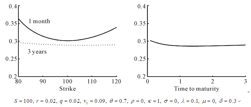 (c)
(c)
 (d)
(d)
Figure 2. Bates model: recreating the implied volatility surface.
where
 (36)
(36)
are square integrable and characteristic functions respectively. In the form (35) we have the forward (−i) Fourier transform. The inverse (+i) Fourier transform is given by
 (37)
(37)
Some Fundamental Properties of Fourier Transforms
Let the Fourier transform of
 be defined as
 then the following fundamental properties hold as follows:
・ Scaling Property
 (38)
(38)
・ Shifting/Translation Property
 (39)
(39)
・ Fourier Transform of Derivatives
 (40)
(40)
This process can be iterated for the nth derivative to yield
 (41)
(41)
Thus, a differentiation converts to multiplication in Fourier space.
・ Convolution Property
 (42)
(42)
Similarly,
 (43)
(43)
・ Linear Property
 (44)
(44)
3.2. The Fast Fourier Transform
The fast Fourier transform is an efficient algorithm for computing the discrete Fourier transform of the form;
 (45)
(45)
where N is typically a power of two. Equation (45) reduces the number of multiplications in the required N summations from an order of N2 to that of , a very considerable reduction. Let p and j be written as binary numbers i.e.
 and
and
 with
with , then (45) becomes
 (46)
(46)
The fast Fourier transform can be described by the following three steps as
 (47)
(47)
The basic idea of the fast Fourier transform is to develop an analytic expression for the Fourier transform of the option price and to get the price by means of Fourier inversion.
The Fast Fourier Transform Method for the Valuation of European Call Option
The Fast Fourier transform method is a numerical approach for pricing options which utilizes the characteristic function of the underlying instrument’s price process. The Fast Fourier transform method assumes that the characteristic function of the log-price is given analytically.
Consider the valuation of European call option. Let the risk neutral density of
 be
be . The characteristic function of this density is given by
 (48)
(48)
The price of a European call option with maturity T and exercise price K denoted by
 is given by
 (49)
(49)
where p is the log of the strike price K i.e.
 (50)
(50)
Substituting (50) into (49) yields
 (51)
(51)
 (52)
(52)
From (52), it is clearly seen that European call price given by (51) is not square integrable function. We consider a modified version of (51) given by
 (53)
(53)
Equation (53) is square integrable in p over the entire real line. Using (36) and (37), we have that
 (54)
(54)
 (54a)
(54a)
Substituting (54a) into (53) and solving further, then we obtain a new call value given by
 (55)
(55)
(56) is a direct Fourier transform and lends itself to an application of fast Fourier transform method. (54) is computed as follows:
 (56)
(56)
Since
 with
with , then the last equation in (56) becomes

Finally we have
 (57)
(57)
Setting , then (57) becomes
 (58)
(58)
The corresponding put values can be obtained by defining ,
,
 ,
,
 with Fourier transform
 (58a)
(58a)
where
 is the Fourier transform of
 . A sufficient condition for
 to be square-integrable is given by
 being finite. This is equivalent to
 .
.
Substituting (58) into (56) with , we have
 (59)
(59)
Similarly, for the price of put option we have that:
 (59a)
(59a)
For the put formula to be well defined, is suffices to choose an appropriate
 in a way that
 .
.
The European call values are calculated using (59). Carr and Madan [2] established that if
 the denominator of (59) vanishes when v = 0, inducing a singularity in the integrand. Since the fast Fourier transform evaluates the integrand at v = 0, the use of the factor
 is required.
Now, we obtain the desired option price in terms of
 using Fourier inversion of the form:
 (60)
(60)
Using basic trapezoidal rule, (60) can be computed numerically as:
 (61)
(61)
where
 (62)
(62)
We are interested in (at the money call values) , the case where the strikes near the underlying spot price of the asset. This type of options is traded most frequently. The fast Fourier transforms method returns N values of p and we then consider a uniform spacing of size
 for the log-strikes around the log-spot price S0 of the form:
 (63)
(63)
Equation (63) gives us log-strike levels ranging from −a to a, where
 (64)
(64)
Substituting (63) and (64) into (61), we have
 (65)
(65)
Now, the fast Fourier transforms method can be applied to xi in (45) provided that . Hence the inte-
gration (60) is an application of the summation (45).
Remark 2:
・ For an accurate integration with larger values of
 we apply basic Simpson’s
 rule weightings into (65) with the condition
 , then the accurate call price which is the exact application of the fast Fourier transform method is obtained as:
 (66)
(66)
where ,
,
 and
and
 is called the Kronecker delta function expressed as:
 (67)
(67)
・ For in-the-money and at-the-money options prices, call values are calculated by an exponential function to obtain square integrable function whose Fourier transform is an analytic function of the characteristic function of the log-price. Unfortunately, for very short maturities, the call value approaches to its non-analytic intrinsic value causing the integrand in the inversion formula of Fourier transforms to vary above and below a mean value and therefore remains tedious to be integrated numerically. We use the alternative approach called the “Time Value Method” proposed by Carr and Madan [2] to mitigate this numerical inconvenience. This approach works with time values only, which is quite similar to the previous approach. But in this context the call price is obtained by means of the Fourier transform of a modified time value, where the modification involves a hyperbolic sine function instead of exponential function.
Let
 represent the time value of out-of-the-money (OTM), that is, for
 we have the call price for
 and for
 we have the put option for
 . Setting
 for simplicity,
 is defined by
 (68)
(68)
where
 is the risk-neutral density of the log-price S and I denotes the indicator function. Let the Fourier transform of
 be defined by
 (69)
(69)
The prices of OTM options can be obtained by the inversion formula of the Fourier transform of (69) of the form
 (70)
(70)
By substituting (68) into (69) and writing in terms of characteristic functions then (69) becomes
 (71)
(71)
There are no issues regarding the integral of this function in (71) as
 or
or , the time value at k tends to zero can get rather steep as T tends to zero and this can make the Fourier transform to be wide and oscillatory. By considering the damping function
 , the time value follows a Fourier inversion:
 (71a)
(71a)
where
 (72)
(72)
Solving (72) further and replace
 by
by , then we have
 (73)
(73)
The use of the fast Fourier transform for calculating out-of-the-money option prices is similar to (66). The only differences are that they replace the multiplication by

with a division by
 and the function call to
 be replaced by a function
 . Hence the formula for out-of-the-money option price is given by
 (74)
(74)
where ,
,
 and
and
 is called the Kronecker delta as given by (67).
3.3. A Closed Form of European Option Pricing under Double Exponential Jump-Diffusion Model with Stochastic Volatility
We derive a closed-form solution of a European call option pricing under double exponential jump-diffusion model with stochastic volatility. The corresponding European put option can be obtained easily by means of put- call parity. For this purpose, we need the following results.
Lemma 3.3.1
Suppose that the variance process vt follows a square root process of the form:
 (75)
(75)
and s1, s2 are any complex, one has
 (76)
(76)
Remark 3:
This result shows that (76) holds because of the affine structure of the variance process.
Lemma 3.3.2 [13]
Suppose the underlying price of the asset follows:
 (77)
(77)
and z is any complex, then
 (78)
(78)
where

Lemma 3.3.3 [35]
Suppose
 is the characteristic function of
 , then
 (79)
(79)
where
 (80)
(80)
Theorem 3.3.4
Let k denote the log of the strike price K,
 and
and
 the desired value of a T-maturity call option with strike ek. Assume that, under martingale probability measure P*, the underlying asset price St with dividend paying stock q and its components are given by:
 (81)
(81)
 is the characteristic function of xT,
 is the probability density of xT given by
 (82)
(82)
then the initial call value
 is written as
 (83)
(83)
where
 represents the real part.
Proof:
From the risk-neutral theory, we have for the case of dividend yield q, the call price of the form
 (84)
(84)
Introducing a change of martingale probability measure from P* to Q* by a Radon-Nikodym derivative, we get

We can write that
 (85)
(85)
Because of the no-arbitrage condition, we can obtain
 (86)
(86)
From the Fourier transform formula, the probability density for this model is given by
 (87)
(87)
Hence,
 (88)
(88)
Therefore, (88) becomes
 (89)
(89)
From (84), (86), (89) and (96), we can obtain the required Theorem 3.3.4.
Remark 4:
For the of non-dividend yield, see [35] .
4. Fast Hilbert Transform in the Theory of Contingent
The Hilbert transform of integrable function f is well defined by the following Cauchy principal value integral
 (90)
(90)
Let the Fourier transform of f be defined as
 (91)
(91)
Suppose that
 is also integrable, a well-known identity in Fourier analysis that is crucial for the application of Hilbert transform is the following;
 (92)
(92)
Here
 is a signum function defined by
 (93)
(93)
Using the translation property of the Fourier transform, it is very easy to obtain the following identities for one dimensional case if
 with
with
 or with
 and
and ;
;
 (94)
(94)
 (95)
(95)
Thus,
 (96)
(96)
Remark 5:
The Hilbert transform on
 is defined as
 (97)
(97)
4.1. Some Fundamental Properties of the Hilbert Transform
It follows directly from the definition of the Hilbert transform that the associated operator is linear. Another slightly less obvious property is that Hilbert transform commutes with translations and positive dilations. For example, let
 be the translation operator defined by
 , and let
 be the dilation operator given by
 for
for . By a simple change of variable, we have that
 (98)
(98)
If we now let R be the reflection operator given by , then we have that
 (99)
(99)
There is no simple formula for the Hilbert transform of product of two functions. However we consider here the special cases of the Hilbert transform of
 and
and
 as follows;
 (100)
(100)
Comparing (90) and (100) we have that

Dividing both sides of the last equation by x and rearrange we have that
 (101)
(101)
The Hilbert transform is an anti-self adjoint operator relative to the duality pairing between
 and dual space
 where p and q are Holder conjugate and
 . Symbolically
 ,
,
 ,
, .
.
4.2. Fast Hilbert Transform Method for the Valuation of European Options
Suppose the dynamics of the underlying price of the asset is given by the following under a given equivalent martingale measure
 (102)
(102)
where Xt is a stochastic process starting at 0. Consider a European put option with exercise price K and maturity T. The payoff function for the European put option is given by
 (103)
(103)
Let the risk neutral expectation of discounted payoff be denoted by PE which is defined as
 (104)
(104)
Substituting (102) and (103) into (104) yields
 (105)
(105)
Equation (105) is called the value of European put option under the risk neutral expectation where r is the risk free interest rate.
The following results enable the derivation of the fast Hilbert transform method for the valuation of European standard put option:
Theorem 4.2.1 [32]
Let
 and
and
 be the cumulative distribution function and the characteristic function of a continuous distribution. Suppose that
 . Then
 (106)
(106)
Remark 6:
This theorem shows that the cumulative distribution function can be computed from the characteristic function through the Hilbert transform.
Theorem 4.2.2 [32]
Let X be a random variable such that
 and
and
 be the characteristic function of X such that
 . Then
 (107)
(107)
Remark 7:
This theorem shows the expectation for the Hilbert transforms representation.
From the two theorems above we obtain the Hilbert representation of European standard put option price as
 (108)
(108)
Similarly European call option price with the same exercise price and maturity can be obtained by means of put call parity of the form;
 (109)
(109)
Substituting the last equation in (108) into (109) we have
 (110)
(110)
The results below summarize the derivation of the Hilbert transform method for the valuation of European options.
Lemma 4.2.3
Suppose the underlying price of the asset satisfies the martingale condition of the form
 . Define the following probabilities
 ,
, . Then the fast Hilbert transform method for the valuation of European
call and put options with non-dividend yield i.e.
 are given by
 and
and
 respectively.
Lemma 4.2.4
Suppose the underlying price of the asset satisfies the martingale condition of the form
 . Define the following probabilities
 ,
, . Then the fast Hilbert transform method for the valuation of European
call and put options with dividend yield q are given by
 and
and
 respectively.
Remark 8:
・ The Lemma 4.2.3 and Lemma 4.2.4 give the fast Hilbert transform for the valuation of European call and put options with non-dividend and dividend yields respectively.
・ The fast Hilbert transform method can also be used for the valuation of timer option which is similar to its European counterpart, except with uncertain expiration date. This type of option is referred to as a barrier style option in the volatility space.
5. Numerical Examples and Discussion of Results
This section presents some numerical examples and discussion of results:
5.1. Numerical Examples
Example 1
Consider the pricing of a contingent claim using fast Fourier transform method with the following parameters
 (111)
(111)
The exercise or strike prices and maturities are generated in MATLAB codes.
The results obtained are shown in the figure below:
Example 2 [35]
We consider European options pricing with double jumps and stochastic volatility using the following parameters:
 (112)
(112)
We compare both the short-term and long-term probability densities of the double exponential-jump diffusion model with a stochastic volatility (SVDEJD), double exponential-jump diffusion model without a stochastic volatility (DEJD) in the context Black-Scholes model (BS) with the maturity time T = 3 months and T = 2 years. The results obtained are shown in the Figure 3.
Example 3
We consider the pricing of “in-the-money (ITM) and at-the-money (ATM)” and “out-of-the-money (OTM)” European call option with the following parameters given:

Figure 3. Pricing of a contingent claim using the fast fourier transform method.
 (113)
(113)
We examine the effects of correlation coefficient, strike price and volatility of volatility; on option values using the fast Fourier transform method. The results generated are shown in the Table 1 and Table 2 for “in-the- money (ITM) and at-the-money (ATM)” and “out-of-the-money (OTM)” European call options respectively.
Example 4 [33]
Consider the pricing of finite-maturity discrete timer options via Monte Carlo method based on 20 Million simulation runs and 800 time steps per year under Heston model and the fast Hilbert transform approach with the following parameters:
 (114)
(114)
The results obtained are shown in Table 3.
5.2. Discussion of Results
From Figure 1(a), Figure 1(b) and Figure 1(c) can see that conditions ,
,
 and
and
 have effect on the heaviness of the left and right tails. When
 , there is an inverse proportion between underlying asset price and volatility, when
 , the skewness is close to zero and when
 , this means that as the underlying asset increases, volatility increases.
Figure 2 shows that adding jumps makes it easier to introduce curvature into the volatility surface, at least for short maturities.
Figure 3 builds the volatility surface based on the parameters of the model and enhances an intuitive understanding of the Heston model. It can be seen from Figure 3 above that there is change in volatility perception. Volatility smile shape has been changed yet volatility for in-the-money and at-the-money options is high and also for out-of-the money options volatility is low. It can be seen from Figure 4 that the long density curves still show significantly different pricing structures between the Black-Scholes model (BS) and its two counterparts (SVDEJD and DEJD). But, more importantly, the densities of the double exponential jump-diffusion model with stochastic volatility and the double exponential jump-diffusion model without stochastic volatility also exhibit different shapes. The SVDEJD density has higher peak and assigns more weight to both the entire lower tail and far upper tail, but less weight to those payoffs than the DEJD [35] .
Table 1 and Table 2 show the effect of correlation coefficient ρ, volatility of volatility
 and strike price K on ITM, ATM and OTM options values using fast Fourier transform. The price of option and the time value for six-month call options associated with volatility of volatility
 and
and
 are relatively close as we can see from Table 1 and Table 2 for ITM, ATM and OTM respectively. The effect of correlation coefficient depends on the relationship between the current underlying price of the asset and strike price. For a positive correlation coefficient, the price of out-of-the-money call option becomes lower. For negative correlation coefficient, the price of in-the-money and at-the-money call options becomes higher. When the correlation coefficient is zero, the effect of volatility of volatility is negligible.
Table 3 shows the comparative results analysis of the fast Hilbert transform and Heston model. It also shows that the relative percentage errors between the fast Hilbert transform and Heston model results are always less than 0.2%. This reveals high level of accuracy of the fast Hilbert transform algorithm.

Figure 4. Comparison of the short-term and long-term probability densities of the double exponential-jump diffusion model (DEJD) without a stochastic volatility, double exponential-jump diffusion model with a stochastic volatility (SVDEJD), in the context Black-Scholes model (BS).

Table 1. The effects of correlation ρ, exercise price K and the volatility of volatility σ “on in-the-money (ITM) and at-the- money (ATM) European options values”.
Table 2. The effects of correlation ρ, exercise price K and the volatility of volatility σ on “out-of-the-money (OTM) European options values”.
Table 3. The comparative results analysis of the fast Hilbert transform approach and Heston model for pricing finite-ma- turity discrete timer call options varying exercise prices K and correlation coefficients ρ.
6. Conclusions
In this work we consider the performance measure of fast Fourier transform for the valuation of contingent claims. The fast Fourier transform method is used because of its advantages when compared to the analytic solution. Using the fast Fourier transform with risk neutral approach provides simplicity in calculations. Heston model is one of the most popular stochastic volatility option pricing models. This model is motivated by the widespread evidence that volatility is stochastic and that the distribution of risky asset return has tails heavier than that of a normal distribution.
The stochastic volatility model incorporates several important features of stock returns. We derive a closed form solution for at-the-money; in-the-money and out-of-the-money European call options using fast Fourier transform method. We also derived a closed form solution for pricing European option under double exponential jump-diffusion with stochastic volatility model. The comparison of the probability densities of the SVDEJD, the Black-Scholes model and the double exponential jump-diffusion model without stochastic volatility shows that SVDEJD model has better performance than the than the two other models on pricing long term options. An analysis of the fast Fourier transform method reveals that the volatility of volatility
 and the correlation coefficient
 have significant impact on option values, especially long-time option, stock returns and negatively correlated with volatility and these negative correlations are important for contingent claims valuation. The numerical example demonstrates high levels of accuracy of the fast Hilbert transform algorithms.
Finally, we can say that fast Fourier transform method is a technique that increases the speed of computation. It is considerably faster than most available methods such as Heston and Bates models. The Hilbert transform method is good for pricing finite-maturity discrete timer options
Cite this paper
Chuma Raphael Nwozo, Sunday Emmanuel Fadugba,, (2015) On Two Transform Methods for the Valuation of Contingent Claims. Journal of Mathematical Finance, 05, 88-112. doi: 10.4236/jmf.2015.52009
References
- Celik, N. (2009) An Application of Fast Fourier Transform Option Pricing Algorithm to the Heston Model. Term Project, Middle East Technical University, Institute of Applied Mathematics.
- Carr, P. and Madan, D. (1999) Option Valuation Using the Fast Fourier Transform. Journal of Computational Finance, 2, 61-73.
- Szymon, B., Kai, D. and Wolfgang Karl, H. (2005) FFT Based Option Pricing. SFB 649 Discussion Paper, No. 2005-011.
- Bakshi, G. and Chen, Z. (1997) An Alternative Valuation Model for Contingent Claims. Journal of Financial Economics, 44, 123-165.
http://dx.doi.org/10.1016/S0304-405X(96)00009-8 - Chen, R.R. and Scott, L. (1992) Pricing Interest Rate Options in a Two-Factor Cox-Ingersoll-Ross Model of the Term Structure. Review of Financial Studies, 5, 613-636.
http://dx.doi.org/10.1093/rfs/5.4.613 - Walker, J.S. (1996) Fast Fourier Transforms. CRC Press, Boca Raton.
- Bakshi, G. and Madan, D.B. (1999) Spanning and Derivative Security Valuation. 34 p.
http://ssrn.com/bstract=153908 - Bates, D. (1996) Jumps and Stochastic Volatility: Exchange Rate Processes Implicit in Deutschemark Options. Review of Financial Studies, 9, 69-108.
http://dx.doi.org/10.1093/rfs/9.1.69 - Scott, L. (1997) Pricing Stock Options in a Jump-Diffusion Model with Stochastic Volatility and Interest Rates: Application of Fourier Inversion Methods. Mathematical Finance, 7, 413-426.
http://dx.doi.org/10.1111/1467-9965.00039 - Heston, S. (1993) A Closed-Form Solution for Options with Stochastic Volatility with Applications to Bond and Currency Options. Review of Financial Studies, 6, 327-343.
http://dx.doi.org/10.1093/rfs/6.2.327 - Merton, R. (1976) Option Pricing When Underlying Stock Returns Are Discontinuous. Journal of Financial Economics, 3, 125-144.
- Zeng, P., Kwok, Y.K. and Zheng, W. (2014) Fast Hilbert Transform Algorithms for Pricing Discrete Timer Options under Stochastic Volatility Models. Working Papers Series, 23 p.
http://ssrn.com/abstract=2465747 - Zeng, P. and Kwok, Y.K. (2013) Pricing Barrier and Bermudan Style Options under Time-Changed Levy Processes: Fast Hilbert Approach. Working Paper of Hong Kong University of Science and Technology.
- Andersen, L.B.G. and Piterbarg, V.V. (2010) Interest Rate Modeling. Volume 1: Foundations and Vanilla Models. Atlantic Financial Press.
- Bakshi, G., Cao, C. and Chen, Z. (1997) Empirical Performance of Alternative Option Pricing Models. Journal of Finance, 52, 2003-2049.
http://dx.doi.org/10.1111/j.1540-6261.1997.tb02749.x - Barndorff-Nielsen, O.E. (1997) Processes of Normal Inverse Gaussian Type. Finance and Stochastics, 2, 4-68.
http://dx.doi.org/10.1007/s007800050032 - Fadugba, S.E. and Nwozo, C.R. (2013) Crank Nicolson Finite Difference Method for the Valuation of Options. Pacific Journal of Science and Technology, 14, 136-146.
- Fadugba, S.E. and Nwozo, C.R. (2014) On the Comparative Study of Some Numerical Methods for Vanilla Option Valuation. Communication in Applied Sciences, 2, 65-84.
- Fadugba, S.E., Ajayi, A.O. and Nwozo, C.R. (2013) Effect of Volatility on Binomial Model for the Valuation of American Options. International Journal of Pure and Applied Sciences and Technology, 18, 43-53.
- Geman, H., Madan, D. and Yor, M. (1998) Asset Prices Are Brownian Motion: Only in Business Time. Working Paper, University of Maryland, College Park.
- Hull, J. and White, A. (1987) The Pricing on Option on Assets with Stochastic Volatilities. Journal of Finance, 42, 281-300.
http://dx.doi.org/10.1111/j.1540-6261.1987.tb02568.x - Lee, R., et al. (2004) Option Pricing by Transform Methods: Extensions, Unification and Error Control. Journal of Computational Finance, 7, 51-86.
- Madan, D.B., Carr, P. and Chang, E.C. (1998) The Variance Gamma Process and Option Pricing. European Finance Review, 2, 79-105.
http://dx.doi.org/10.1023/A:1009703431535 - McCulloch, J.H. (1978) Continuous Time Processes with Stable Increments. Journal of Business, 51, 601-620.
- Nwozo, C.R. and Fadugba, S.E. (2012) Some Numerical Methods for Options Valuation. Communications in Mathematical Finance, 1, 51-74.
- Nwozo, C.R. and Fadugba, S.E. (2012) Monte Carlo Method for Pricing Some Path Dependent Options. International Journal of Applied Mathematics, 25, 763-778.
- Nwozo, C.R. and Fadugba, S.E. (2014) On the Accuracy of Binomial Model for the Valuation of Standard Options with Dividend Yield in the Context of Black-Scholes Model. IAENG International Journal of Applied Mathematics, 44, 33-44.
- Nwozo, C.R. and Fadugba, S.E. (2014) On the Strength and Accuracy of Advanced Monte Carlo Method for the Valuation of American Options. International Journal of Mathematics and Computation, 25, 27-41.
- Nwozo, C.R. and Fadugba, S.E. (2014) Performance Measure of Laplace Transforms for Pricing Path Dependent Options. International Journal of Pure and Applied Mathematics, 94, 175-197.
http://dx.doi.org/10.12732/ijpam.v94i2.5 - Nwozo, C.R. and Fadugba, S.E. (2014) Mellin Transform Method for the Valuation of Some Vanilla Power Options with Non-Dividend Yield. International Journal of Pure and Applied Mathematics, 96, 79-104.
- Stein, E. and Stein, J. (1991) Stock Price Distribution with Stochastic Volatility: An Analytic Approach. Review of Financial Studies, 4, 727-752.
http://dx.doi.org/10.1093/rfs/4.4.727 - Lin, X. (2010) The Hilbert Transform and Its Application in Computational Finance. Ph.D. Thesis, University of Illinois at Urbana-Champaign.
- Xu, J. (2003) Pricing and Hedging under Stochastic Volatility. Master’s Thesis, Peking University, Beijing.
- Black, F. and Scholes, M. (1973) The Pricing of Options and Corporate Liabilities. Journal of Political Economy, 81, 637-659.
http://dx.doi.org/10.1086/260062 - Zhang, S. and Wang, L. (2011) A Fast Fourier Transform Technique for Pricing European Options with Stochastic Volatility and Jump Risk. Mathematical Problems in Engineering, 2012, Article ID: 761637.
http://dx.doi.org/10.1155/2012/761637