ABSTRACT

This paper discusses the pricing problem of credit default swap in the fractional Brownian motion environment. As credit default swap is exposed to both the interest rate risk and the default risk, we assume that the default intensity of a firm depends on the stochastic interest rate and the default states of counterparty firms. The interest rate risk is reflected by the fractional Vasicek interest rate model. We model the firm’s default intensity under the looping default model and derive the pricing formulas of risky bonds and credit default swap.

Keywords:Credit Default Swap; Bond; Contagious Risk; Fractional Vasicek Interest Rate Model; Looping Default

1. Introduction

Credit risk is one of the main risks in the financial industry. It is very important for the financial industry to manage credit risk effectively. Since credit default swap (CDS) appeared, it soon became one of the most important derivatives to manage credit risk because of its great advantages. However, as the rapid expansion of credit default swap market, some concealed contradictions exposed gradually, such as the United States subprime crisis and the European sovereign debt crisis. They make people realize that credit derivatives bring convenience and contain huge risk at the same time, especially contagious risk. Therefore, the valuation and pricing of credit derivatives have called for more effective models according to the real market.

Until now, there have been mainly two basic models: the structural model and the reduced-form model. In the first model, the firm’s default is governed by the value of its assets and debts, while the default in the reduced-form model is governed by the exogenous factor. However, the information of the firm’s assets is usually unknown and the problem of the valuation of credit derivatives involving the jump-diffusion process is still difficult to get explicit results in the event of defaulting before the maturity date in the structural model. Therefore, comparing with the structural approach, the reduced-form approach is more flexible and tractable in the real market. In this paper, we will price the bonds and CDS in the reduced-form models.

The reduced-form model was pioneered by [1,2]. They introduced exogenous mechanism to describe the firm’s default. Their models considered the default as a random event which was controlled by an exogenous intensity process. Later, [3] extended their models and considered the default intensity which satisfied the Cox process. [4] further discussed the jump affine intensity, and so on.

In the reduced-form model, suppose that is a filtered probability space satisfying the usual conditions, where (is large enough but finite), and is an equivalent martingale measure under which discounted securities’ prices are martingales. On, there is a -valued process where represents the economy-wide state variable. Denote and, where represents the default process of company. When

first jumps from 0 to 1, we call the company defaults and denote be the default time of company.

Thus, where is the indicator function. This paper consider that the interest rate is the only state variable and that the default intensity is stochastic. The default times of company can be defined as

(1)

where is the unit exponential random variable. The distributions of conditional default probability of company are given by

(2)

The fractional Brownian motion was firstly defined and studied by Kolmogorov in Hilbert space, and was named to the Wiener spiral. Because the fractional Brownian motion has the properties of self-similarity and long-range dependence and many phenomena in financial market show these properties in some certain, the fractional Brownian motion becomes a very suitable tool in different applications such as mathematical finance.

However, for the Hurst index, the fractional Brownian motion is neither a Markov process, nor a semimartingale, and we can not use the usual stochastic calculus to analyze it. Worse still after a pathwise integration theory for fractional Brownian motion was developed by [5,6], it was proved that their market mathematical models driven by the fractional Brownian motion could have arbitrage ([7]). Later, after the development of a new kind of integral based on the Wick product (see [8,9]) called fractional Ito integral, it was proved ([9]) that the corresponding Ito type fractional Black-Scholes market has no arbitrage. In the same paper, a formula for the price of a European option at was derived. Based on these conclusions, [10] proved some results regarding the quasi-conditional expectation and obtained a risk-neutral valuation formula of the European option for every before the maturity date. All the conclusions build a solid theoretical foundation for its application in the financial field.

This paper also consider the Hurst index. We will give the following definitions and theorems without the proofs. The details can be found in [10].

Definition 1 Let be measurable. Then if

where,.

Definition 2 (Fractional Brownian motion) Let be the filtered probability space satisfying the usual conditions. is a constant. The fractional Brownian motion with Hurst index is a continuous Gauss process, which satisfies 1);

2).

Definition 3 (Quasi-conditional expectation) Let, be the random distribution space with inductive topology, then the quasi-conditional expectation of with respect to

is defined by

(3)

where. For simplicity, we denote it as.

Definition 4 (Quasi-martingale) Suppose that is an adapted stochastic process with respect to

. If, then we say that is a quasi-martingale.

From the above definitions, it is easy to prove the following theorems:

Theorem 1 ([10])

1) is a quasi-martingale;

2) Let, then is a quasi-martingale;

3) Let, then is a quasi-martingale.

The interest rate has an important influence on pricing credit derivatives, especially after the fixed interest rate is replaced by the floating interest rate, and the impact will be more important. From the point of time, the interest rate also has the characteristics of the fractional Brownian motion. Therefore, [11] used the fractional Brownian motion to describe the interest rate process which was the fractional Vasicek interest rate model and priced the European option. In this paper, we also consider the Vasicek interest rate model:

(4)

where is the fractional Brownian motion which describes the market risk, is the standard deviation which represents the stochastic volatility, parameter is the long-term average of interest rate, and represents the speed of recovery that returns to from the deviation value of the long-term average. The interest rate has the following explicit solution:

(5)

where is the interest rate value at time 0. follows the normal probability distribution with mean and the variance. Thus, is the normal stochastic variable with mean and the variance.

To make the formula simple, we suppose that the face value of bond is 1 dollar. The default-free bond’s price was obtained in [11] as following:

Theorem 2 ([11]) Let be the time-t value of the default-free bond with the maturity date. The interest rate is derived by the fractional Brownian motion as above. The price of market risk is, then

(6)

where

2. Bonds’ Pricing under the Looping Default Model

[12] firstly proposed the model of credit contagion to account for concentration risk in large portfolios of defaultable securities (DL Model). Later, [13] thought the traditionally structural and reduced-form models were full of problems because they all ignored the firm’s specific source of credit risk. They made use of the Davis’s contagious model and introduced the concept of counterparty risk which was from the default of firm’s counterparties. In their models, they paid more attention to the primary-secondary framework in which the intensity of default was influenced by the economy-wide state variables and the default state of the counterparty. Beside these, there are also other similar applications such as [14,]">15] and so on. In recent years, [16,]">17] further allowed the stochastic interest rate to follow an jump-diffusion process and studied the pricing problem of bonds and CDS in details. Based on the obtained conclusions, we will price the bonds and CDS with the fractional Vasicek interest rate in the looping default framework.

In the following, we only consider the case with two firms: firm and firm. Their defaults are mutually influenced and both correlated with the market interest rate. We assume their intensity processes respectively satisfy some linear relations below:

(7)

(8)

where, , , are positive constants, , are the real numbers which satisfy, We will give the defaultable bond’s price without the proof (see [13]). Let.

Lemma 1 ([13]) Suppose that the bond issued by firm has the maturity date and the recovery rate. Let the default time be, the default intensity be and the interest rate be, then

(9)

Now, we calculate the conditionally marginal distributions of default time and in [0, T] before deriving the prices of bonds. To avoid the looping influences, we firstly apply the change of measure to get the joint conditional distributions of and. We define two firm-specific probability measures by

(10)

Under the new measure, the intensity for

Thus, the default model can be simplified and the calculation of the default probabilities and bonds’ prices will be relatively easy.

Theorem 3 Let and be the default times of firm and. Assume the interest rate and the default intensities, satisfy (4), (7) and (8). If no defaults occur up to time, then the joint conditional distribution of and on is given by the following:

when and

when

Proof. Let When, from the properties of quasi-conditional expectation ([10])we have

where denotes the quasi-conditional expectation under probability measure

When, the intensity of becomes under, so we have

Denote Hence, we proceed to calculate the quasi-conditional expectation in the first term of the above joint conditional distribution as follows.

Then, substituting the obtained two quasi-conditional expectation into the joint conditional distribution, we can deduce the conclusion of the theorem when When, the calculating process is similar to above. We omit it.

Corollary 1 Let and be the default times of firm and. Suppose that the default intensities and satisfy (7) and (8). If no defaults occur up to time, then the conditionally marginal distributions of and on are given by

(11)

(12)

Proof. We can obtain the corollary from Theorem 3, so omit the process.

Now, we apply the above results to price the bonds issued by firm and in the looping default framework. We firstly give the other form of pricing formula for the bond. Later, we will price the bonds based on this formula.

Lemma 2 ([13]) The defaultable bond price can also be expressed as

(13)

In this paper, we will not consider the risk from the recovery rate. Therefore, without loss of generality, we suppose that the recovery rates and the face value of bond is 1 dollar.

Theorem 4 Assume the interest rate follows the fractional Vasicek model and the default intensities and satisfy (7) and (8). If no defaults occur up to time, then the time- prices of bonds issued by firm, with the same maturity date are respectively given by

(14)

(15)

where

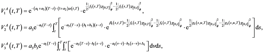
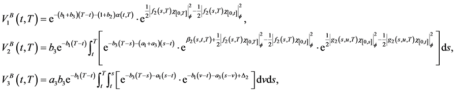
where

Proof. Firstly, according to the pricing formula on fractional quasi-martingale in Hu and Ksendal (2003) and Lemma 2, we can obtain the price of bond issued by firm at time on is

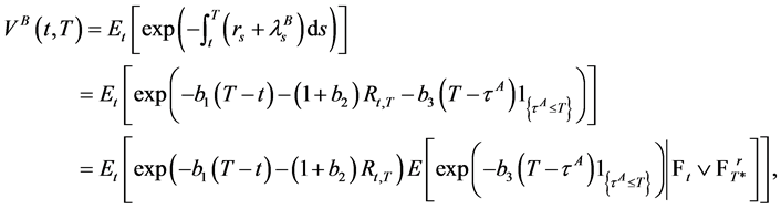
where

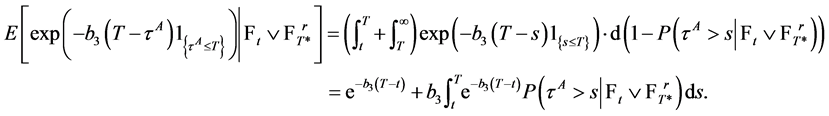
By Corollary 1, we have

From the equation of, we find that the key step is to calculate the three quasi-conditional expectation, and

. By (5), we show

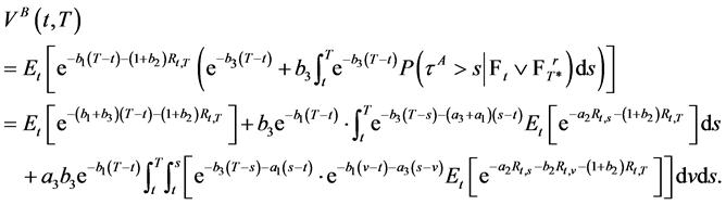
Further, substituting it into and by the definition of quasi-martingale and (2) in Theorem 1, we show that

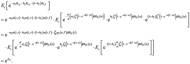
In the above equality,

Similarly,

then

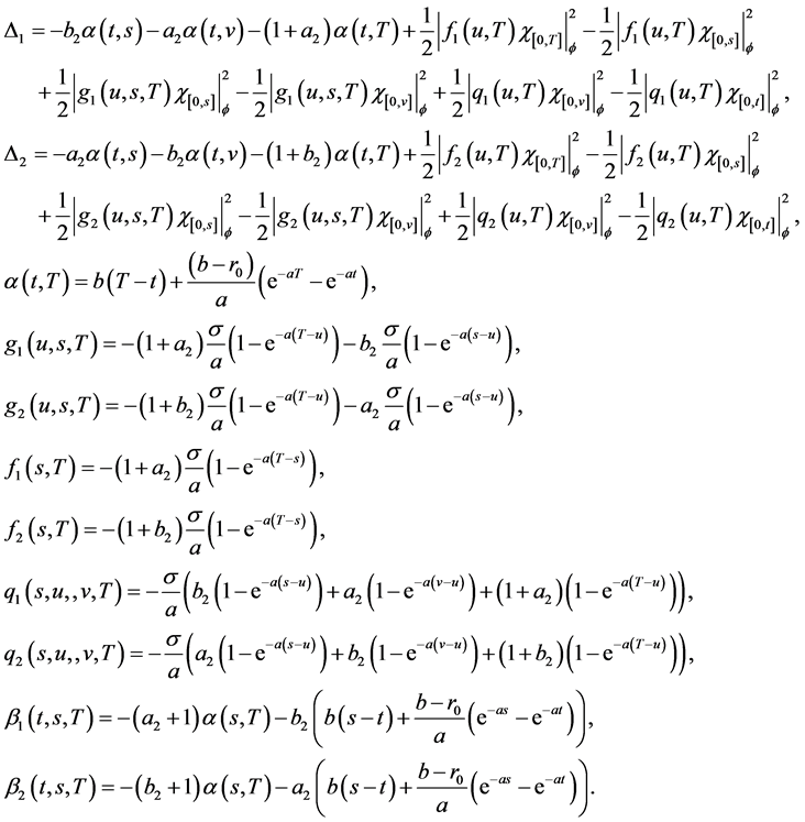
where

Therefore,

When, we apply the properties of quasi-conditional expectation and obtain

Finally, we substituting the above quasi-conditional expectations into. We show that (15) holds. The pricing formula (14) of bond issued by firm can be derived though the similar proving process of. Hence, we omit it. The proof is complete.

3. CDS’s Pricing

In this section, we apply the results in section 2 to price CDS related to the zero coupon bond issued by firm. Firm holds a bond issued by the reference firm with the maturity date. To seek protection against the possible loss, firm buys a default swap with the maturity date from firm on condition that firm gives the payments to seller at a fixed swap rate in time while seller promises to compensate buyer for the loss caused by the default of firm at a certain rate. Each party has the obligation to make payments until its own default. The source of credit risk may be from three parties: the issuer of bond, the buyer of CDS and the seller of CDS.

In the following, we discuss a simple situation which only contains the default risk from reference firm and the CDS’s seller. At the same time, to make the calculation convenient, we suppose the recovery rate of the bond issued by firm is zero and the notional is 1 dollar. In the event of firm’s default, firm compensates firm for 1 dollar if he doesn’t default, otherwise 0 dollar.

Now, we give some notations. Denoted the swap rate by a constant and interest rate by. Let the default times of firm and be with the intensity and with the intensity respectively. We analyze the values of two legs: contingent leg and premium leg. The time-0 market value of buyer’s payments to seller is

the time-0 market value of firm’s promised payoff in case of firm’s default is

Then, in accordance with the arbitrage-free principle, we obtain

(16)

Theorem 5 Suppose the interest rate satisfies fractional vasicek interest rate model and the intensities and satisfy

Then, if no defaults occur up to time, the swap rate has the following expression

(17)

where are the simple forms of (6) and (14) in Theorem 2 and Theorem 4, and

Proof.

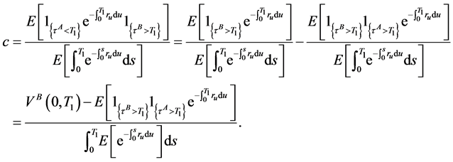
To derive the swap rate of CDS in the looping default framework, we define a firm-specific probability measure by

then

Substituting the quasi-conditional expectation into the above formula of the swap rate, we deduce (17).

4. Conclusions

This paper discusses the pricing problem of defaultable bonds and CDS in the fractional Brownian motion environment. In our model, we consider the case that the defaults of the firms are mutually influenced. The default intensity is correlated with the counterparty’s default and the interest rate following fractional Vasicek model, which is more realistic.

In fact, we consider that the source of credit risk may be from the issuer of bond and the seller of CDS. In this case, there are also four cases for the defaults of firm and firm:

Case 1. The defaults of firm and firm are mutually independent conditional on the interest rate;

Case 2. Firm is the primary party whose default only depends on the risk-free interest rate (the only economy state variable) and the firm is the secondary party whose default depends on the interest rate and the default state of firm;

Case 3. Firm is the primary party and the firm is the secondary party;

Case 4. The defaults of firm and firm are mutually contagious (looping default).

In this paper, we only discuss the complex case 4 but the other cases are relatively simple which can be considered as the special situations of case 4. The pricing problem in case 2 has been studied in the other paper. In addition, we can try to discuss the more general situations. For example, we can consider the case that the impact of one firm’s default to the other firm’s default is attenuated over time or the relevant recovery rate is stochastic. In a word, the contagious model of credit security is very necessary to be further discussed in the future.

5. Funds

It is supported by the National Natural Science Foundation of China (No:11271259); the TianYuan Special Funds of the National Natural Science Foundation of China (No:11326170); Innovation Program of Shanghai Municipal Education Commission (No:13YZ125); Funding scheme for training young teachers in Shanghai Colleges (ZZshjr12010).

REFERENCES

- R. A. Jarrow and S. M. Turnbull, “Pricing Derivatives on Financial Securities Subject to Credit risk,” Journal of Finance, Vol. 50, No. 1, 1995, pp. 53-85. http://dx.doi.org/10.1111/j.1540-6261.1995.tb05167.x
- J. D. Duffie and K. J. Singleton, “Modeling Term Structures of Defaultable Bonds,” Review of Financial Studies, Vol. 12, No. 4, 1999, pp. 687-720. http://dx.doi.org/10.1093/rfs/12.4.687
- D. Lando, “On Cox processes and credit risky securities,” The Review Derivatives Research, Vol. 2, No. 2, 1998, pp. 99-120. http://dx.doi.org/10.1007/BF01531332
- D. Duffie, et al., “Transform Analysis and Asset Pricing for Affine Jump Diffusions,” Econometrica, Vol. 68, No. 6, 2000, pp. 1343-1376. http://dx.doi.org/10.1111/1468-0262.00164
- S. J. Lin, “Stochastic Analysis of Fractional Brownian Motion, Fractional Noises and Applications,” SIAM Review, Vol. 10, 1995, pp. 422-437.
- L. Decreusefond and A. S. Ustunel, “Stochastic Analysis of the Fractional Brownian Motion,” Potential Analysis, Vol. 10, 1999, pp. 177-214. http://dx.doi.org/10.1023/A:1008634027843
- L. C. G. Rogers, “Arbitrage with Fractional Brownian Motion,” Mathematical Finance, Vol. 7, No. 1, 1997, pp. 95-105. http://dx.doi.org/10.1111/1467-9965.00025
- T. E. Duncan, Y. Hu and B. Pasik-Duncan, “Stochastic Calculus for Fractional Brownian Motion, I. Theory,” SIAM Journal on Control and Optimization, Vol. 38, No. 2, 2000, pp. 582-612. http://dx.doi.org/10.1137/S036301299834171X
- Y. Hu, B. Øksendal and A. Sulem, “Optimal Portfolio in a Fractional Black-Scholes Market,” In: S. Albeverio, et al., Eds, Mathematical Physics and Stochastic Analysis, World Scientific Singapore City, 2000.
- Y. Hu and B. Øksendal, “Fractional White Noise Calculus and Application to Finance,” Infinite Dimensional Analysis, Quantum Probability and Related Topics, Vol. 6, No. 1, 2003, pp. 1-32.
- W. L. Huang, X. X. Tao and S. H. Li, “Pricing Formulae for European Option under the Fractional Vasicek Interest Rate Model,” Acta Mathematica Sinica (in Chinese), Vol. 55, No. 2, 2012, pp. 219-230.
- M. Davis and V. Lo, “Infectious Defaults,” Quantitive Finance, Vol. 1, No. 4, 1999, pp. 382-387. http://dx.doi.org/10.1080/713665832
- R. A. Jarrow and F. Yu, “Counterparty Risk and the Pricing of Defaultable Securities,” Journal of Finance, Vol. 56, No. 5, 2001, pp. 1765-1799. http://dx.doi.org/10.1111/0022-1082.00389
- S. Y. Leung and Y. K. Kwork, “Credit Default Swap Valuation with Counterparty Risk,” Kyoto Economic Review, Vol. 74, No. 1, 2005, pp. 25-45.
- Y. F. Bai, X. H. Hu and Z. X. Ye, “A Model for Dependent Default with Hyperbolic Attenuation Effect and Valuation of Credit Default Swap,” Applied Mathematics and Mechanics (English Edition), Vol. 28, No. 12, 2007, pp. 1643-1649. http://dx.doi.org/10.1007/s10483-007-1211-9
- R. L. Hao and Z. X. Ye, “The Intensity Model for Pricing Credit Securities with Jumpdiffusion and Counterparty Risk,” Mathematical Problems in Engineering, Vol. 10, 2011, pp. 1-16.
- R. L. Hao and Z. X. Ye, “Pricing CDS with Jump-Diffusion Risk in the Intensity-Based Model,” Advances in Intelligent and Soft Computing, Vol. 100, 2011, pp. 221-229. http://dx.doi.org/10.1007/978-3-642-22833-9_26