ABSTRACT

We investigate the impact of delegated portfolio management on asset prices in a noisy rational equilibrium model. Asset prices in our model are linear in fund managers’ private signals and in realized supply shocks. We show that equilibrium expected returns 1) decrease as the proportion of fund managers increase in the economy; 2) decrease as the precision of fund managers’ signals increase’ and 3) increase as the fund managers’ contingent fees increase.

1. Introduction

Today, most investors delegate their investment decisions to financial professionals. For example, equity holdings through delegated management (such as pension funds and mutual funds) in the US market have increased from 7.2 percent in 1950 to more than 49 percent in 2002, whereas the proportion held directly by individuals has decreased from about 90 percent to slightly below 40 percent over the same period.[1]

In his presidential address, Allen [2] provides reasons why investors delegate the portfolio decision process: 1) professional investment analysis possesses economies of scale; 2) investors may recognize their own limited knowledge and capacity for information dissemination/ processing and therefore hire a professional manager; and 3) a professional manager might be able to steer free from the behavioral biases that individual investors otherwise have been shown to be susceptible to.

However, financial institutions and professional fund managers are influenced by incentives that are not fully captured by standard models in finance^1,2. Therefore, the significant increase of ownership of equities under delegated management raises the question: how does this form of ownership affect asset prices?

In behavioral models of asset pricing, people have nonstandard preferences and/or form beliefs that are not based on rational information processing³. However, by turning to professional managers an investor faces an agency problem. Delegated investing implies that relative asset prices depend on the utility functions of agents, not the utility functions of investors. Because of asymmetric information and different incentives present in delegated decision making, the utility functions of agents are different from the ones of consumers.

There are several differences between the delegated portfolio management problem considered here and the standard agency problem: 1) the delegated portfolio management problem is one of information acquisition rather than direct performance. Consequently, in the delegated portfolio management problem the fund manager exerts effort to obtain a private (noisy) signal, and thereafter makes portfolio decisions based on the signal received. 2) Contrary to a typical agency problem where the agent only chooses whether or not to take action and cannot influence the size/strength of his response, the fund manager has full discretion in his portfolio decisions and controls both return and variance of the portfolio.

The dominant portion of the theoretical literature in delegated management focuses on partial equilibrium settings represented by a game between an investor (principal) and a portfolio manager (agent) where asset prices and returns are taken as given. However, an important aspect of delegated portfolio management concerns the impact of this agency relationship on asset prices. Indeed, the type of compensation contracts or incentives agreed upon between investor and manager influence the equilibrium at the aggregate level. For example, if fund managers underperform relative to their peer group (or some other benchmark) investors may transfer their capital to a better performing fund (fund chasing). This mechanism typically results in fund managers being afraid of taking too much risk relative to the peer group. They may end up investing in similar stocks to their peers; driving up the prices of these “peer group popular” stocks and driving down the prices of “peer group unpopular” stocks. These types of effects have been studied to some extent in the literature, see for example, [6-14].

This paper studies how delegated portfolio management affects asset prices. Our model is inspired by the single-security noisy rational expectations equilibrium of [15-17]. It is also related to the models of [18,19].

The outline of this paper is as follows. In section 2, we introduce a simple economy with two risky assets and a risk-free bond with two types of agents, fund managers and investors, both with CARA preferences – but with different final wealth. Fund managers receive a private noisy signal about future payoffs of the risky assets whereas investors only have access to the public information and information revealed from asset prices in equilibrium. Then, in sections 3 and 4, we derive the portfolio decisions and demand functions for each agent, and show that the noisy rational expectation equilibrium exists where asset prices are linear in fund managers’ signals and in realized supply shocks. We discuss the impact of delegated portfolio management on the equilibrium risk premiums and on the cross-section of returns. Section 5 concludes and provides possible extensions of this model.

2. Model

The noisy rational expectations framework of [15-17] inspires our model.  This framework centers on the idea that uninformed agents use the equilibrium asset price as an informative signal about asset returns and extract some of the information that the informed agents possess.

2.1. Economy and Preferences

We consider a two period model where market participants choose their portfolio allocation “today” (t = 0) and assets are liquidated and paid off “tomorrow” (t = 1). The economy consists of a continuum of two groups of agents: investors and fund managers. Investors endowed with an initial wealth of W₀ can choose either to manage their portfolio themselves or delegate the investment decision to a fund manager. Fund managers have no independent wealth and are not allowed to borrow. We assume there are as many fund managers as there are delegating investors and that each delegating investor is matched with one fund. After investors make the decision to selfmanage or to delegate, the proportion of fund managers and self-managing investors are μ and 1-μ, respectively. We will refer to these two groups as the “fund managers” and the “investors”; and we use superscript M for fund managers and I for investors to distinguish functions and variables that are specific to these two groups.

We assume all agents in our model have CARA preferences with risk aversion parameter ρ, so that the expected utility of a final payoff of W becomes

.

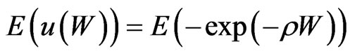2.2. Asset Structure

There are three assets in the economy, a risk-free bond and two risky assets. The bond, normalized to have a price of 1 at t = 0, yields a certain gross return of R at t = 1 and has perfect elastic supply. The two risky assets have a price at t = 0 of with independent random payoffs at t = 1 of with mean and precision; that is

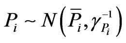
where i = 1, 2⁴. We assume that markets clear. Then, as we will see, the prices today of the risky assets can be determined endogenously. The per capita supplies of the risky assets are independent and normally distributed,

where. The supply is never observed, but agents who possess information, as defined below, can back it out from equilibrium prices. We interpret this random supply as the presence of noise traders in the economy and remark that 1) the role of random supply shocks is to prevent information from being fully revealing to uninformed agents; and 2) a positive expected per capita supply implies that in equilibrium, some agents will hold the risky assets.

2.3. Information Structure

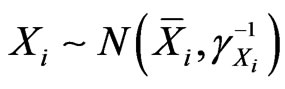
All agents in our economy have a common prior distribution of the final payoffs of the risky assets. However, at t=0 fund managers obtain independent and normally distributed private signals for each asset⁵

where

.

this signal is unobservable to investors. They know only that fund managers have superior information in terms of them receiving a normally distributed signal on each risky asset in the economy.

2.4. Fund Manager Compensation.

Fund managers’ final wealth depends on their compensation. Today, the most common compensation of professional managers is a fixed percentage of the portfolio value. For example, fees earned by mutual fund managers are proportional to assets under management⁶. For hedge funds, it is more common that compensation schemes reward managers by the portfolio’s total return in absolute terms or relative to a particular benchmark. The compensation may also feature a floor or a cap, often based on the value of assets under management⁷.

In this paper we use the linear compensation contract defined by a pair (f, k), where f is the fixed fee paid to the fund manager regardless of portfolio performance and k, 0 ≤ k ≤ 1, the fraction of the final portfolio value paid to the fund manager⁸. We will refer to the fraction k as the “contingent fee.” In other words, if W is the final portfolio value then the linear contract implies a compensation to the fund manager of

.

Consequently, the final wealth of the delegating investor becomes

.

3. Portfolio Choice

Given the model set up described in the previous section, next we determine agents’ demand functions and then solve for equilibrium.

We denote by, the demands of an agent a, where and 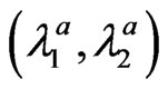are his allocations to the risk-free bond and the two risky assets, respectively. Since asset returns and payoffs in our model are normally distributed, the expected utility for agent a with a final payoff of can be expressed as

.

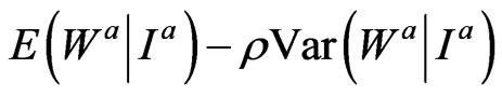The budget constraint for self managing investors is

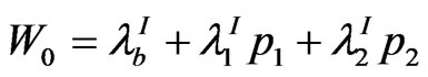and their final payoff is the random variable

.

Substituting the budget constraint into investors’ final payoff gives

.

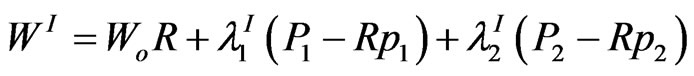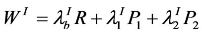
Similarly, fund managers’ final payoff becomes

.

3.1. Fund Manager Demand

Maximizing the expected utility of the fund managers’ final payoff, their demand functions become

.

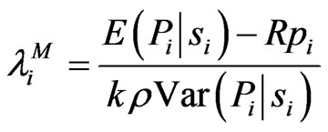
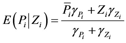
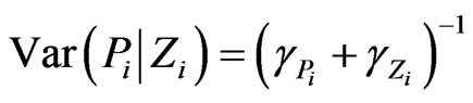
Calculating the conditional expectation and variance by Bayes’ rule, we obtain

and

.

After substituting these expressions into the fund managers demand function, we get

.

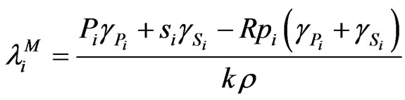We observe that the fund managers’ demand increases when the contingent fee k (the proportion of final portfolio value received by fund managers as compensation) decreases. Intuitively, the contingent fee changes fund managers’ risk aversion from to, and thus fund managers are expected to trade more aggressively when their contingent compensation is smaller. The fund manager demand function also captures the case when fund managers do not receive signals; setting 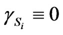in the expression above yields

.

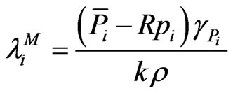3.2. Investor Demand

Similar to fund managers, investors’ demand functions take the form

where I^I denotes the information set available to investors. While investors do not observe the private signals available to fund managers, they condition upon that in equilibrium market prices convey information. With the knowledge that fund managers have private signals and their associated distributions, investors rationally infer how these signals will affect the demands of the fund managers and consequently also equilibrium prices. In order to learn from prices, the investors must conjecture a price function and, in the rational expectations equilibrium, this conjecture must be correct. We assume investors conjecture the linear price function

where and are the signal and the supply for assets i, and the coefficients and are determined in equilibrium⁹.

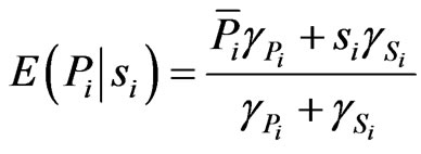
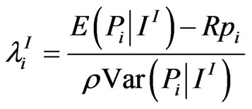
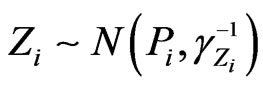
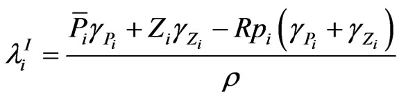
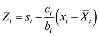
To calculate the expectation and the variance conditional on the conjectured price, we first introduce the random variable defined by

.

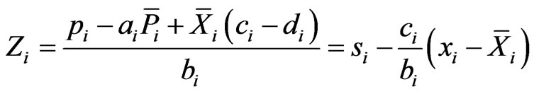Since the only uncertainty in this random variable stems from p_i, we note that conditioning on is equivalent to conditioning on the price conjecture. We observe that

where

and therefore by Bayes’ rule

and

.

Substituting this into the investors’ demand functions yields

.

4. Equilibrium Prices and Demands

Here, we establish equilibrium prices for our model and derive some implications of such prices. In particular, we discuss how the delegated portfolio management industry affects the equity premium and the cross-section of returns. We also look at how changes in the economic environment and the information structure impact investor and fund manager demands. We start with our main result in this section, Proposition 1.

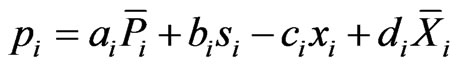
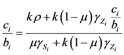
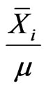
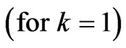
Proposition 1: Given the three asset economy described above with a fraction of μ fund managers under contract (f, k) and a fraction of 1-μ investors, then there exists a noisy rational expectations equilibrium at time t = 0 such that asset prices are given by

where i = 1,2 and

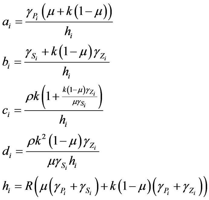
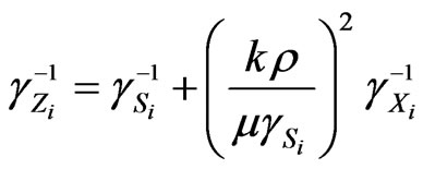
Finally, the precision of Z_i is

.

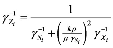Proof: First, we note that market clearing implies that

.

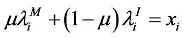Substituting fund managers’ and investors’ demand functions, we obtain

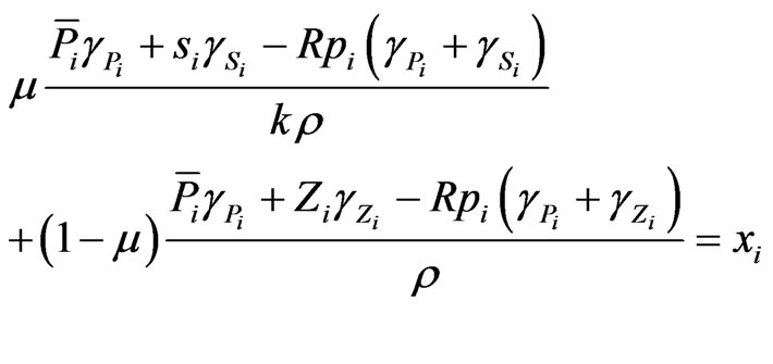
Substituting

and solving for p_i yields

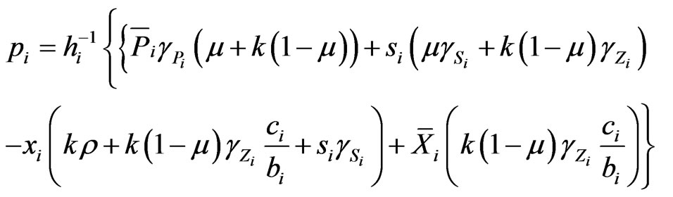
We observe it must hold that

from which it follows that

.

Therefore,

and

The proposition now immediately follows.

The next proposition summarizes some properties of the equilibrium prices established in Proposition 1.

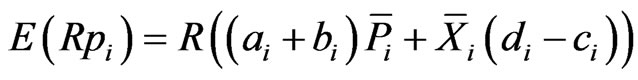
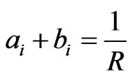
Proposition 2: The equilibrium expected return on the risky assets are given by

.

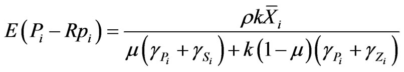Furthermore, we have that

1) Equilibrium expected returns are decreasing functions in the proportion of fund managers μ in the economy, that is

;

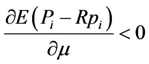2) Equilibrium expected returns are increasing functions in the risk aversion parameter ρ, that is

;

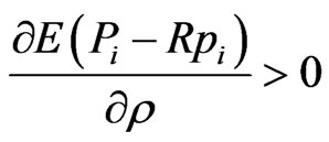3) Equilibrium expected returns are decreasing functions in the precision of the fund managers’ signal, that is

;

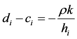
4) Equilibrium expected returns are decreasing functions in the precision of the assets’ payoff, that is

;

5) Equilibrium expected returns are increasing functions in the fraction k of the final portfolio value paid to the fund manager, that is

;

and

6) Equilibrium expected returns are not affected by changes in the precision of the assets’ supply, that is

.

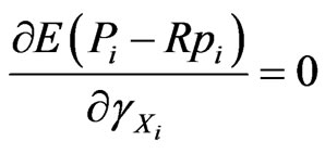
Proof: Using equilibrium prices from Proposition 1, we have

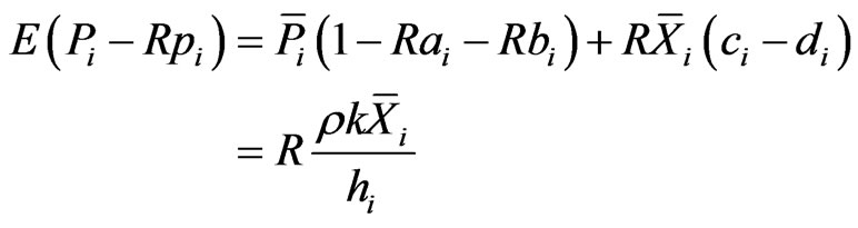
since

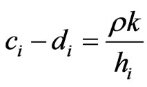
and

.

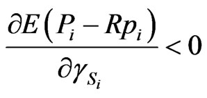
The proofs of (a)-(f) are similar. Here we show (a): It’s easy to see that 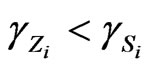for all admissible values of k and μ. In other words, the precision of the signals investors infer are always smaller than the signals fund managers receive. Consequently,

.

We emphasize that Proposition 2 implies a positive risk premium for the risky assets. In particular, since these assets are risky, agents demand compensation for holding them in equilibrium. The risk premium decreases as the fraction of fund managers increases (part (a)) because fund managers are more informed and their information is partly revealed in equilibrium.

Jagannathan, McGrattan and Scherbina [23] show that the equity premium has declined significantly since the 1970s. They estimate the premium averaged around 7 percent during the period 1926-70 and thereafter decreased to about 0.7 percent. The authors argue that it is difficult to rationalize a shrinking equity premium by a permanent shift in investor preferences. Instead, they suggest that institutional changes occurred in the US stock market that causes a permanent shift in stock returns. Fama and French [24] reach similar conclusions. Through a dividend growth model, they show that the equity premium has shrunk from about 4.17 percent during the period 1872-1950, to about 2.55 percent for the half-century 1951-2000. We understand these views as consistent since delegated management in the US market increased from 7.2 percent in 1950 to more than 49 percent in 2002. At the same time, the proportion of investments held directly by individuals decreased from about 90 percent to slightly below 40 percent [1].

Proposition 2 also holds implications for the crosssection of returns. In particular, all else equal, the equilibrium risk premium is higher for the asset where the precision of fund managers’ signals is lower (part (c)) or where fund investment is lower (part (a)). This can be interpreted in several different ways. For example, the largest fund managers tend to focus their research on the subset of stocks where capacity and liquidity are sufficiently high (typically, large-cap stocks) thereby being able to acquire more precise signals for these stocks.

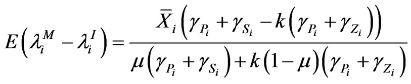
The results from Proposition 2 are consistent with the empirical findings of [25] who argue that the demand pressure for risky assets (in particular large-cap stocks) is a direct consequence of the growth of institutional investors. They also show from their data that the last decade’s decrease in the small-cap premium is due to the same effect. Lakonishok, Shleifer and Vishny [3] suggest that pension fund managers are biased towards “glamour” stocks, that is, stocks that are easy to justify buying. Glamour stocks with proven track records of consistent earnings growth may attract investors because nobody would doubt them as “good” companies. In our model, we can loosely interpret glamour stocks as assets where fund managers’ signals and assets’ payoffs have higher precision. They suggest further that the increased demand for equity by institutions and unsophisticated individuals who equate profitability with potential capital gains have made these stocks overpriced. In our simple set up, we can derive the following relationship between fund manager and investor demands:

Proposition 3: Suppose and denote fund manager and investor demands for asset i as derived above. Then, the average difference in demand is positive and given by

.

Proof: Direct calculation shows that

Using the equilibrium price from Proposition 1, we have

.

Now, observing that

and

the proposition follows.

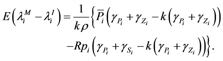
We note the average difference in demand between fund managers and investors is a decreasing function in the fraction μ of fund managers in the economy and fund managers’ contingent fee k. In particular, this difference decreases from

to

.

the high fund manager demand for low compensation levels (small k) raises the question of leverage. From the perspective of an investor in a fund, it makes sense to impose some form of leverage constraints. We note that, in practice, mutual funds are subject to short selling and borrowing/margin constraints that naturally limit fund manager demand.

In this model, demand differences occur because fund managers and investors do not have the same beliefs about assets’ expected return and variance. In contrast, in the incomplete market model of [26], different demands arise because not all agents are aware of all assets in the economy. Here, both fund managers and investors hold the same assets and thus bear idiosyncratic risk, but choose to do so in different proportions. If we take into consideration that fund managers will overweight stocks with “good” prospects and underweight them with “bad” prospects, then since the investors will hold the remainder, they will end up underweighting “good” stocks and overweighting “bad” stocks.

5. Conclusions and Extensions

The model presented in this paper is inspired by the single-security noisy rational expectations equilibrium of [15-17]. It is also related to [18,19]. Our main contribution is in using a noisy rational expectations equilibrium framework to study the impact of delegated portfolio management on asset prices.

Using an exponential-normal set up, we modeled a simple economy consisting of two types of agents, fund managers and investors. Fund managers were assumed to receive a private noisy signal about future payoffs of the risky assets, whereas investors only have access to the public information and information revealed from asset prices in equilibrium. Our main findings are as follows:

1) We proved that a partially revealing equilibrium exists where asset prices are linear in fund manager signals and in realized supply shocks.

2) Studying the impact on equilibrium expected returns from delegated portfolio management, we showed that these risk premiums: a) decrease as the proportion of fund managers increase in the economy; b) decrease as the precision of fund managers’ signals increase; and c) increase as the fund managers’ contingent fees (the fraction of the final portfolio value paid to the fund manager as compensation) increase.

3) The result under 2) b) has some implications for the cross-section of returns. All else being equal, the equilibrium risk premium is higher for assets where the precision of fund managers’ signals is lower.  This we can interpret, for example, in the following way: when the largest fund managers focus their research on the subset of stocks where capacity and liquidity are sufficiently high (typically, large-cap stocks) they acquire more precise signals for these stocks. Through their higher demand in these assets, asset prices increase thereby decreasing future returns.

4) Due to asymmetric information, fund managers and investors hold the same stocks, but with different exposure to idiosyncratic risk. In particular, the average difference in fund manager and investor demands for a particular asset is positive, and is a decreasing function in the fraction of fund managers in the economy and the fund managers’ contingent fee.

In closing, we discuss several possible extensions.

5.1. Distributional Assumptions

In our framework we assumed that payoffs of the risky assets and fund managers’ signals are independent and identically distributed—that is, all risk is idiosyncratic. A natural extension is to introduce correlations between assets and between signals. There are several directions in which this can be done. Following [20], one can assume that asset payoffs are distributed normally and satisfy a general variance-covariance matrix and that private signals are simply risky asset payoffs plus noise. One can then proceed as proposed in [27] by positing a factor model setting where noisy signals are available to fund managers for these systematic factors. Unfortunately, these two frameworks allow for explicit closed form solutions for equilibrium prices only in special cases.

One way to proceed is to use a set up like the working paper of [28]. They investigate the effects of private information and diversification on risk premiums in a noisy rational expectations model where payoffs of the risky assets obey a factor structure and private signals, These provide information on both systematic factors and idiosyncratic risks. One obtains solutions for equilibrium prices in this multi-asset exponential-normal framework.

5.2. Finite and Infinite Asset Economies

Under homogeneous beliefs/information the implications of risk premiums are known from arbitrage pricing theory (APT). Under asymmetric information, the impact of private signals on risk premiums in large economies are less understood. Delegated portfolio management provides a natural mechanism with which fund managers incorporate private signals into the economy. It may be of interest to study an extension of the factor model discussed in the previous paragraph where the number of assets approaches infinity. Then one might determine the conditions that lead to linear pricing relationships.

5.3. Investment Decisions

In our simple model we made the assumption that investors decide either to delegate or self-manage their portfolio. In practice, this is an unrealistic assumption. Investors typically hold a proportion of their investments in delegated mutual funds and another in self-managed stocks.

5.4. Heterogeneity

For simplicity, we have assumed all agents are homogeneous and thus have identical risk aversion. Preliminary results, not reported here, show the basic results from this model carry over to a heterogeneous economy.

5.5. Participation, Short Selling and Borrowing/Margin Constraints

We assumed that fund managers’ participation constraints are satisfied. As observed in Sections 3 and 4, fund manager demand increases as the contingent compensation k decreases. To keep their risk exposure constant as contingent compensation decreases, fund managers will increase their leverage. Since most funds (for example, mutual funds) are subject to short selling and borrowing/margin constraints, incorporating these in a model (to limit fund manager demand) seems a natural extension. However, these constraints lead to nonlinear equilibrium prices that must be solved by numerical techniques (see, for example, the noisy rational expectations model in [29]).

5.6. Information Costs and the Size of the Delegated Portfolio Management Business

Precise information comes at a cost. A natural extension is first to model the cost of information acquisition in our model and endogenize this decision by solving for the optimal signal acquiring strategy as a function of contingent fees and other parameters (for the single risky asset case, see for example, [17]). Next, one might solve for the fraction of fund managers in the economy endogenously.

This would be particularly interesting in a multi-asset economy—where assets and signals are correlated—in which information is more expensive for certain types of assets, and could produce new understandings of delegated portfolio management on the cross-section of returns. This might also provide a greater comprehension of why so many different mutual funds and mutual fund families are available in the marketplace. In a setting of this type, we might even examine the relationship between fund specialization and contingent fees.

5.7. Incomplete Market Economies

It may also be interesting to study a multi-security model with uninformed (or irrational) investors and rational fund managers. Uninformed investors consider a small part of the investable universe in the sense of [26], and calculate their demands conditional on the prices they observe only on these assets. Fund managers, on the other hand, condition on all available assets and therefore benefit from cross-security aggregation. This model would exploit the differences between multi-security equilibrium prices, obtained along the lines of [20] and single-security equilibrium prices derived in this paper.  

5.8. Sharing of Information

We observe in the marketplace that many larger mutual fund companies offer a whole menu of mutual funds in different flavors. In order to better understand the relationship between mutual funds in a fund family, one must model how they share information: 1) in which cases do fund managers share information; 2) do they collude in determining management fees; and 3) what is the optimal equilibrium relationship between contingent fees and the size of mutual fund families?

REFERENCES

NOTES

¹See, for example, [3].

²We note that most mutual fund shareholders own their funds through financial intermediaries such as a professional financial advisor, defined contribution retirement plan, brokerage firm, banks, insurance company, or mutual fund supermarket. The mutual fund holdings of individuals that are held directly with the fund company have decreased from 28 percent in 1982 to about 15 percent in 2003 (see, [4]). However, this “double” or “nested” agency situation is outside the scope of this paper.

³For a survey of behavioral finance, see [5].

⁴In our setup rational expectations equilibrium prices of risky assets are independent of each other, and no cross-security information aggregation is present. In other words, there is no difference between singlesecurity equilibrium prices (as in [16]), and the multi-security equilibrium prices (as in [20]). In future work we intend to generalize this model. We provide a discussion of these extensions in Section 5.

⁵We ignore any costs for the informative signals in this paper. Nevertheless, introducing a convex cost does not significantly change our results.

⁶According to [21] only about 1.7 percent of US mutual funds used fulcrum fees in 1999. Reference [22] identified fulcrum fees in only 27 of 370 funds studied; the remaining funds charged a fixed fraction of assets under management.

⁷By the 1970 amendment to the Investment Company Act of 1940, mutual funds must use a form of incentive fee known as a ‘‘fulcrum fee.’’ The (symmetric) incentive fee centers around a benchmark, increases the fees for performance above the benchmark, and decreases the fees for performance below the benchmark. In practice, the size of the incentive fees has a floor and cap. In contrast, the (asymmetric) incentive fee structure used by hedge funds and other private partnerships is typically non-negative, has a high watermark, uses zero (or cash) as a reference benchmark, and does not have a cap.

⁸For expositional simplicity, we assume that the contract has been chosen such that the fund managers’ participation constraint (e.g. a constraint of the form) is satisfied. We do this to avoid having to distinguish between the two different cases of the Karush-Kuhn-Tucker conditions in which the constraint is either binding or non-binding at the optimum.

⁹A direct application of the standard noisy rational expectations equilibrium framework of [16] and [15] proves the existence of this linear price function.

REFERENCES

- NYSE, “Institutional Investors,” Factbook, New York Stock Exchange, New York, 2003.
- F. Allen, “Do Financial Institutions Matter?” Journal of Finance, Vol. 56, No. 4, 2001, pp. 1165-1175. http://dx.doi.org/10.1111/0022-1082.00361
- J. Lakonishok, A. Shleifer and R. W. Vishny, “The Structure and Performance of the Money Management Industry,” Microeconomics, Vol. 1992, 1992, pp. 339-391.
- Investment Company Institute, “Ownership of Mutual Funds through Professional Financial Advisers,” Research Fundamentals, Vol. 14, No. 3, 2005.
- N. Barberis and R. Thaler, “A Survey of Behavioral Finance,” In: G. M. Constantinides, M. Harris and R. M. Stulz, Eds., Handbook of the Economics of Finance, Elsevier Science, Oxford, 2004, pp. 1051-1121.
- D. S. Scharfstein and J. C. Stein, “Herd Behaviour and Investment,” American Economic Review, Vol. 80, No. 3, 1980, pp. 465-479.
- D. W. Diamond and R. E. Verrecchia, “Optimal Managerial Contracts and Equilibrium Security Prices,” Journal of Finance, Vol. 37, No. 2, 1982, pp. 275-287. http://dx.doi.org/10.2307/2327326
- R. T. Ramakrishnan and A. V. Thakor, “Moral Hazard, Agency Costs, and Asset Prices in a Competitive Equilibrium,” Journal of Financial and Quantitative Analysis, Vol. 17, No. 4, 1982, pp. 503-532. http://dx.doi.org/10.2307/2330905
- R. T. Ramakrishnan and A. V. Thakor, “The Valuation of Assets under Moral Hazard,” Journal of Finance, Vol. 39, No. 1, 1984, pp. 229-238. http://dx.doi.org/10.1111/j.1540-6261.1984.tb03870.x
- N. Arora and H. Ou-Yang, “Explicit and Implicit Incentives in a Delegated Portfolio Management Problem: Theory and Evidence,” Unpublished, 2001.
- E. Goldman and S. L. Slezak, “Delegated Portfolio Management and Rational Prolonged Mispricing,” Journal of Finance, Vol. 58, No. 1, 2003, pp. 283-311. http://dx.doi.org/10.1111/1540-6261.00525
- H. Ou-Yang, “Optimal Contracts in a Continuous-Time Delegated Portfolio Management Problem,” Review of Financial Studies, Vol. 16, No. 1, 2003, pp. 173-208. http://dx.doi.org/10.1093/rfs/16.1.173
- B. Cornell and R. Roll, “A Delegated-Agent Asset-Pricing Model,” Financial Analysts Journal, Vol. 61, No. 1, 2005, pp. 57-69. http://dx.doi.org/10.2469/faj.v61.n1.2684
- S. A. Ross, “Markets for Agents: Fund Management,” In: B. N. Lehmann, Ed., Legacy of Fischer Black, University Press, Oxford 2005, pp. 96-124.
- S. J. Grossman and J. E. Stiglitz, “On the Impossibility of Informationally Efficient Markets,” American Economic Review, Vol. 70, No. 3, 1980, pp. 393-408.
- M. F. Hellwig, “On the Aggregation of Information in Competitive Markets,” Journal of Economic Theory, Vol. 22, 1980, pp. 477-498. http://dx.doi.org/10.1016/0022-0531(80)90056-3
- R. E. Verrecchia, “Information Acquisition in a Noisy Rational Expectations Economy,” Econometrica, Vol. 50, No. 6, 1982, pp. 1415-1430. http://dx.doi.org/10.2307/1913389
- M. O’Hara, “Presidential Address: Liquidity and Price Discovery,” Journal of Finance, Vol. 58, No. 4, 2003, pp. 1335-1354. http://dx.doi.org/10.1111/1540-6261.00569
- D. Easley and M. O’Hara, “Information and the Cost of Capital,” Journal of Finance, Vol. 59, No. 4, 2004, pp. 1553-1583. http://dx.doi.org/10.1111/j.1540-6261.2004.00672.x
- A. R. Admati, “A Noisy Rational Expectations Equilibrium for Multi-Asset Securities Markets,” Econometrica, Vol. 53, No. 3, 1985, pp. 629-658. http://dx.doi.org/10.2307/1911659
- E. J. Elton, M. J. Gruber and C. R. Blake, “Incentive Fees and Mutual Funds,” Journal of Finance, Vol. 58, No. 2, 2003, pp. 779-804. http://dx.doi.org/10.1111/1540-6261.00545
- J. H. Golec, “Empirical Tests of a Principal-Agent Model of the Investor-Investment Advisor Relationship,” Journal of Financial and Quantitative Analysis, Vol. 27, No. 1, 1992, pp. 81-95. http://dx.doi.org/10.2307/2331299
- R. Jagannathan, E. R. McGrattan and A. Scherbina, “The Declining US Equity Premium,” Federal Reserve Bank of Minneapolis Quarterly Review, Vol. 24, No. 4, 2000, pp. 3-19.
- E. F. Fama and K. R. French, “The Equity Premium,” Journal of Finance, Vol. 57, No. 2, 2002, pp. 637-659. http://dx.doi.org/10.1111/1540-6261.00437
- P. A. Gompers and A. Metrick, “Institutional Investors and Equity Prices,” Quarterly Journal of Economics, Vol. 116, No. 1, 2001, pp. 229-259. http://dx.doi.org/10.1162/003355301556392
- R. C. Merton, “A Simple Model of Capital Market Equilibrium with Incomplete Information,” Journal of Finance, Vol. 42, No. 3, 1987, pp. 483-510. http://dx.doi.org/10.1111/j.1540-6261.1987.tb04565.x
- A. R. Admati, “On Models and Measures of Information Asymmetries in Financial Markets,” PhD, Yale University, New Haven, 1982.
- J. Hughes and J. Liu, “Private Information, Diversification and Asset Pricing,” Unpublished, 2005.
- E. Ozdenoren and K. Yuan, “Feedback Effects and Asset Prices,” Journal of Finance, Vol. 63, No. 4, 2006, pp. 1939-1975. http://dx.doi.org/10.1111/j.1540-6261.2008.01378.x
NOTES
1See, for example, [3].
2We note that most mutual fund shareholders own their funds through financial intermediaries such as a professional financial advisor, defined contribution retirement plan, brokerage firm, banks, insurance company, or mutual fund supermarket. The mutual fund holdings of individuals that are held directly with the fund company have decreased from 28 percent in 1982 to about 15 percent in 2003 (see, [4]). However, this “double” or “nested” agency situation is outside the scope of this paper.
3For a survey of behavioral finance, see [5].
4In our setup rational expectations equilibrium prices of risky assets are independent of each other, and no cross-security information aggregation is present. In other words, there is no difference between singlesecurity equilibrium prices (as in [16]), and the multi-security equilibrium prices (as in [20]). In future work we intend to generalize this model. We provide a discussion of these extensions in Section 5.
5We ignore any costs for the informative signals in this paper. Nevertheless, introducing a convex cost does not significantly change our results.
6According to [21] only about 1.7 percent of US mutual funds used fulcrum fees in 1999. Reference [22] identified fulcrum fees in only 27 of 370 funds studied; the remaining funds charged a fixed fraction of assets under management.
7By the 1970 amendment to the Investment Company Act of 1940, mutual funds must use a form of incentive fee known as a ‘‘fulcrum fee.’’ The (symmetric) incentive fee centers around a benchmark, increases the fees for performance above the benchmark, and decreases the fees for performance below the benchmark. In practice, the size of the incentive fees has a floor and cap. In contrast, the (asymmetric) incentive fee structure used by hedge funds and other private partnerships is typically non-negative, has a high watermark, uses zero (or cash) as a reference benchmark, and does not have a cap.
8For expositional simplicity, we assume that the contract has been chosen such that the fund managers’ participation constraint (e.g. a constraint of the form ) is satisfied. We do this to avoid having to distinguish between the two different cases of the Karush-Kuhn-Tucker conditions in which the constraint is either binding or non-binding at the optimum.
9A direct application of the standard noisy rational expectations equilibrium framework of [16] and [15] proves the existence of this linear price function.