Journal of Mathematical Finance
Vol.3 No.1(2013), Article ID:28126,23 pages DOI:10.4236/jmf.2013.31002
Some Explicitly Solvable SABR and Multiscale SABR Models: Option Pricing and Calibration
1Department of Mathematics and Information Technology, University of Camerino, Camerino, Italy
2Department of Economics, University of Verona, Verona, Italy
3Department of Management, University Politecnica Marche, Ancona, Italy
4Department of Mathematics, “G. Castelnuovo”, University of Rome “La Sapienza”, Rome, Italy
Email: lorella.fatone@unicam.it, francesca.mariani@univr.it, m.c.recchioni@univpm.it, f.zirilli@caspur.it
Received September 20, 2012; revised November 16, 2012; accepted November 29, 2012
Keywords: Multiscale Stochastic Volatility Models; Option Pricing; Calibration Problem; FX Data
ABSTRACT
A multiscale SABR model that describes the dynamics of forward prices/rates is presented. New closed form formulae for the transition probability density functions of the normal and lognormal SABR and multiscale SABR models and for the prices of the corresponding European call and put options are deduced. The technique used to obtain these formulae is rather general and can be used to study other stochastic volatility models. A calibration problem for these models is formulated and solved. Numerical experiments with real data are presented.
1. Introduction
In this paper a multiscale SABR model that describes the time dynamics of forward prices/rates is presented. This model generalizes the well known SABR model introduced in 2002 by Hagan Kumar, Lesniewski, Woodward in [1]. Under some hypotheses on the correlation structure of the model studied when we restrict our attention to the normal and lognormal multiscale SABR models it is possible to derive explicit (closed form) formulae to express the transition probability density functions of the stochastic processes implicitly defined by the models and of the prices of the corresponding European call and put options. Using the technique developed to derive the transition probability density function of the multiscale SABR model we deduce new explicit formulae for the transition probability density function of the normal and lognormal SABR models presented in [1]. Specifically we show that the transition probability density functions of the normal and lognormal SABR models (with no assumptions on the correlation structure of the models) can be written as the inverse Fourier transform of explicitly known kernels. Moreover we show that for the multiscale models (under some assumptions on the correlation structure of the models) the corresponding multiscale transition probability density functions can be expressed as the inverse Fourier transform of the product of two copies of these kernels. This property is interesting since it can be used to define easy to solve multiscale versions of other stochastic volatility models.
The multiscale SABR model introduced in this paper is motivated by the behaviour in the financial markets of equity prices, interest rates and currency exchange rates. In several circumstances empirical studies have shown that the dynamics of these quantities is described more satisfactorily by models that use at least two factors to describe the volatility dynamics than by models that use only one factor (see, for example, [2-4] and the reference therein). In [5-7] it has been shown that a generalized Heston model, that uses two stochastic volatilities varying on two different time scales, leads to satisfactory forecasts of the asset prices and of the corresponding European option prices. The prices considered in [5-7] are the S&P 500 index, the associated European call and put option prices and some spot electric power prices. These findings motivate the use in the multiscale SABR model of two factors (i.e. two stochastic volatilities) varying on two different time scales to describe the volatility of the forward prices/rates variable. We limit our attention to “normal” and “lognormal” SABR and multiscale SABR models. In these models the instantaneous variation of the forward prices/rates depends only on the volatility or on the volatilities (“normal” models) or on the volatility or on the volatilities times the prices/rates itself (“lognormal” models). These models are special cases of more general SABR models where the variation of the forward prices/rates depends on the product between a sufficiently smooth function of the forward prices/rates and the volatility or the volatilities. Usually this function is chosen in the family of functions  where
where  is a real variable and
  is a parameter. That is the SABR models considered depend on the parameter
 ,
,  , the normal models correspond to the choice
  and the lognormal models correspond to the choice
 .
.
Let  and
and  be respectively the sets of real and of positive real numbers and let
  be a real variable that denotes time. Let us define the multiscale SABR model. To the forward prices/rates described by the stochastic process
 ,
,  , we associate two stochastic volatilities given by the stochastic processes
 ,
,  ,
, . The dynamics of the stochastic process
 ,
,  ,
,  ,
,  , is defined by the following system of stochastic differential equations:
 (1)
(1)
 (2)
(2)
 (3)
(3)
where the quantities ,
,  , and
, and  are real positive constants such that
  and
and . The fact that
 ,
,  ,
,  , vary on different time scales is expressed by the condition
 . When the condition
  holds it is likely to observe abrupt changes in the forward rates/prices variable. The processes
 ,
,  ,
,  ,
,  , are standard Wiener processes such that
 , and
, and ,
,  ,
,  ,
,  ,
,  , are their stochastic differentials. The correlation structure of the model is defined by the following assumptions:
 (4)
(4)
 (5)
(5)
 (6)
(6)
 (7)
(7)
 (8)
(8)
 (9)
(9)
where  denotes the expected value of
  and the quantities
  are constants known as correlation coefficients. The autocorrelation coefficients of the previous stochastic differentials are equal to one. When the model is multiscale (i.e. when
 ) the meaning of the assumptions (4)-(9) is that the stochastic differentials on the right hand side of (1)-(3) associated to the two (long and short) time scales are independent.
The Equations (1)-(3) are equipped with the initial conditions:
 (10)
(10)
 (11)
(11)
 (12)
(12)
where ,
,  ,
,  , are random variables that we assume to be concentrated in a point with probability one. For simplicity we identify the random variables
 ,
,  ,
,  , with the points where they are concentrated. We assume
 ,
, .
.
The stochastic differential Equations (1)-(3), the initial conditions (10)-(12), the assumptions on the correlation coefficients (4)-(9) and the conditions on the coefficients ,
,  ,
,  , define the multiscale SABR model. This model generalizes the SABR model introduced in 2002 by Hagan, Kumar, Lesniewski, Woodward [1] that is defined by the following stochastic differential equations:
 (13)
(13)
 (14)
(14)
where  and
and . The coefficients
  and
and  of (13), (14) are known respectively as
  -volatility and as volatility of volatility. Moreover
 ,
,  ,
,  , are standard Wiener processes such that
 ,
,  ,
,  , are their stochastic differentials and we have:
 (15)
(15)
where  is a constant called correlation coefficient. The Equations (13) and (14) are equipped with the initial conditions:
 (16)
(16)
 (17)
(17)
where  and
and  are random variables that we assume to be concentrated in a point with probability one and that, for simplicity, we identify with the points where they are concentrated. Moreover we assume that
 .
.
Note that for  the assumption
  with probability one implies that
  with probability one for
 . A similar statement holds for
  and
and ,
, .
.
We consider the normal and the lognormal SABR and multiscale SABR models. These models are obtained from the previous ones choosing respectively in Equations (13) and (1)  (normal models) or
  (lognormal models). When we consider the lognormal models we assume that
 . In the lognormal models the assumption
  with probability one implies that
  with probability one for
 . Under the assumptions (4)-(9) for the normal and lognormal SABR and multiscale SABR models the transition probability density functions associated to the state variables of these models are expressed via integral formulae with explicitly known integrands. In this sense the normal and lognormal models are explicitly solvable. The SABR and multiscale SABR models with
 ,
,  can be studied using the following approaches: numerical methods, series expansions in the parameter
  or hybrid methods. The last approach combines series expansions and numerical methods. The SABR models with
 ,
,  can be studied using integral formulae involving hypergeometric functions for their transition probability density functions [8]. The models with
  deserve special attention. These models will be studied elsewhere.
We begin our analysis with the study of the normal multiscale SABR model (see Section 2) for three reasons. The first reason is that under the previous hypotheses on its correlation structure the normal multiscale SABR model can be solved explicitly. The second reason is that the normal multiscale SABR model can be considered as an improvement not only of the normal SABR model but also of SABR models with  different from zero, sufficiently small. In fact the use of two volatilities makes the normal multiscale model more “flexible” than the SABR models. For example the normal multiscale SABR model reproduces both balanced and skewed probability distributions of prices/rates and can forecast satisfactorily the option prices even when the options considered have strike price near to zero and are at the money. In these circumstances the normal SABR model fails to explain the observed prices. The third reason is that in the class of SABR models parametrized by
 ,
,  , the normal models are the simplest ones and their study is useful to understand the other models. For example in Section 3 we use the results obtained in the study of the normal models to study the lognormal models.
The explicit formulae of the transition probability density functions associated with the normal and lognormal models are one (SABR models) or three dimensional (multiscale SABR models) integrals of explicitly known integrands. The formulae are closed form and “easy to use” in the sense that their numerical evaluation can be done with elementary methods. These formulae are used to derive explicit (closed form) formulae for the corresponding prices of European call and put options. The option pricing formulae are integrals of explicitly known integrands. Due to the special form of the integrands the numerical evaluation of the multi-dimensional integrals involved in the formulae of the transition probability density functions and of the option prices can be done very efficiently with ad hoc quadrature rules.
Moreover from the formula for the normal multiscale SABR transition probability density function we derive a formula for the transition probability density function of the normal SABR model. This formula is expressed as a one dimensional integral of a (regular) explicitly known integrand, is an elementary formula that can used instead of the formula deduced in [9] (Formula (120) in [9]). This last formula (Formula (120) in [9]) is based on the McKean formula for the heat kernel of the Poincaré plane. In a similar way a new formula for the transition probability density function of the lognormal SABR model is deduced. This last formula is a special case of an explicit, “easy to use” formula for the transition probability density function of the stochastic process implicitly defined by the Hull and White model [10] when there is a possibly nonzero correlation between the stochastic differentials appearing on the right hand side of the forward prices/rates and volatility equations. These are two interesting formulae since up to now in the case of nonzero correlation for the transition probability density functions of the lognormal SABR model and of the Hull and White model only asymptotic expansions in the correlation coefficient were known (see for example [10,11] and the references therein). The results relative to the Hull and White model will be presented elsewhere. The formulae presented in this paper are obtained using the Fourier transform, the method of separation variables and the results of Yakubovic [12] about the Lebedev Kontorovich Transform.
A calibration problem for the normal and lognormal SABR and multiscale SABR models is considered. These models are calibrated using option price data, the option pricing formulae mentioned above and the least squares method. The calibration problem is formulated as a constrained optimization problem for the least squares error function. Given the forward prices/rates the calibrated models are used to forecast option prices. We discuss some numerical experiments with real data where observed and forecast option prices are compared. These experiments confirm the validity of the procedure used to forecast option prices, of the calibration procedure and of the models presented. In particular they make possible a comparison between SABR and multiscale SABR models that shows when the use of the multiscale SABR models is justified.
The real data used in the calibration problem and in the forecasting experiments are discrete time observations of the euro/US dollar (EUR/USD) exchange rate (futures prices), of the futures prices of the USA five year interest rate swap and of the prices of the corresponding European put and call options (i.e. European foreign exchange options on EUR/USD futures prices and options on USA five year interest rate swap futures). That is we consider Foreign eXchange (FX) data and interest rates data. Note that forward/futures prices are quantities stated in the contracts stipulated to buy or to sell currencies in a future date and that they remain unchanged during the life time of the contracts. For the convenience of the reader let us recall some facts about the derivatives mentioned above. A foreign exchange option is a derivative that gives to the owner the right but not the obligation to exchange a given quantity of money denominated in one currency into money denominated in another currency in a specified date at a pre-agreed exchange rate. Exchange rate derivatives are widely traded and serve different needs, for example, they serve the needs of firms active in the international trade arena that want to reduce their exposure to exchange rate variations. The USA five year interest rate swap exchanges semiannual interest rate payments at the fixed rate of 4% per floating interest rate payments based on 3-month LIBOR interest rate. These swaps are widely traded. In fact they are excellent tools for duration management and asset/ liability gap management for bank treasuries, insurers and financial services companies. Note that the use of futures prices/rates instead of forward prices/rates in our numerical experiments is due to the fact that only the latter ones are over the counter prices. Moreover recall that when during the time period considered the risk free interest rates are deterministic forward and futures prices/ rates coincide (see [13], Proposition 3.1 and [14]).
The numerical experiment on the EUR/USD exchange rate shows that, once calibrated using call and put option prices relative to a given date, the normal multiscale SABR model, given the asset price at the time of the forecast, is able to produce forecasts of call and put option prices that outperform those obtained with the normal SABR model. Note that the values of the parameters  and
and  of the normal multiscale model obtained in the calibration differ of approximately a factor two. This means that the calibrated multiscale model has really a multiscale behaviour and as a consequence the interpretation of the data benefits from the presence of the second time scale.
In the next experiment the lognormal models are used to interpret interest rate swaps data. In this case the futures price has abrupt changes so that the improvement in the data interpretation obtained introducing the multiscale model is significant. In particular when the lognormal multiscale SABR model is considered the values of the parameters  and
and  obtained in the calibration differ for about a factor two. The results obtained on the interest rate swap data with the lognormal models confirm the findings of the experiments on the EUR/ USD exchange rate data with the normal models. Finally the stability of the parameter values obtained in the calibration is investigated. It is shown that calibrating the models daily with the option price data collected in one day during a period of about two months (that is calibrating the models approximately forty times) the models parameters obtained remain substantially unchanged during the two months period. Recall that there are approximately twenty trading days in a month.
The website: http://www.econ.univpm.it/recchioni/ finance/w14 contains some auxiliary material including animations that help the understanding of this paper. A more general reference to the work of the authors and of their coauthors in mathematical finance is the website: http://www.econ.univpm.it/recchioni/finance.
The remainder of the paper is organized as follows. In Section 2 we study the normal SABR and multiscale SABR models. In Section 3 we study the lognormal SABR and multiscale SABR models. In Section 4 we formulate a calibration problem for these models and we present a numerical method to solve it. In Section 5 a procedure that, given the asset prices at the time of the forecast, forecasts option prices using the calibrated models is presented. The calibration and forecasting procedures are applied to study real data. Currency exchange rates and interest rates derivatives data and the corresponding option price data are studied. The forecast option prices are compared with the prices actually observed. The comparison shows the relevance of the multiscale SABR models. Finally in Section 6 some conclusions are drawn.
2. The Normal SABR and Multiscale SABR Models
Let us consider the normal multiscale SABR model. This model is obtained choosing  in (1), (2), (3) and is given by the following stochastic differential equations:
 (18)
(18)
 (19)
(19)
 (20)
(20)
with the initial conditions:
 (21)
(21)
 (22)
(22)
 (23)
(23)
where ,
,  ,
,  , are random variables that we assume to be concentrated in a point with probability one. The quantities
 ,
,  , are positive constants such that
 . Moreover we assume that conditions (4)-(9) hold. In a similar way starting from (13), (14), (16), (17) and choosing
  in (13) we can write the normal SABR model.
Let us consider the transition probability density function of the stochastic process ,
,  ,
,  ,
,  , implicitly defined by (18)-(23), that is the probability density function of having
 ,
,  ,
,  given the fact that
 ,
,  ,
,  , when
 ,
,  ,
,  , and
, and . Note that when
  we must choose
 ,
,  ,
, . This transition probability density function is denoted with


 ,
, . Note that the values
 ,
,  of the forward prices/rates vary on the real axis, and that they can be negative. We denote with
  ,
,  ,
,  , the function

 , considered as a function of the variables
 . The function
  is the solution of the Fokker Planck equation:
 (24)
(24)
with the initial condition:
 (25)
(25)
and appropriate boundary conditions. The symbol  denotes the Dirac’s delta and in (25) the operator
  is given by:
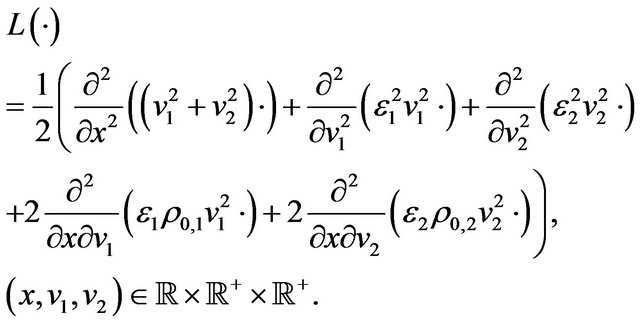 (26)
(26)
The operator  defined in (26) depends on the assumptions (4)-(9). The Fokker Planck Equation (24) is a linear parabolic partial differential equation whose elliptic part is degenerate on the boundary of its domain of definition, that is it is degenerate when
  or
or  and
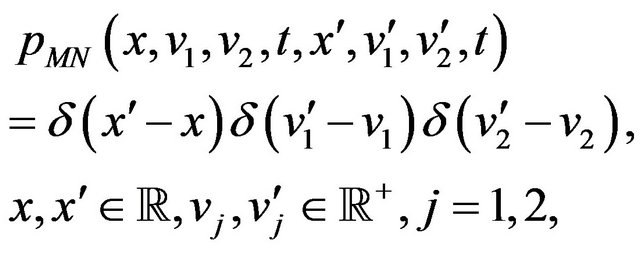
and . Problems (24), (25) are completed with appropriate boundary conditions. The degeneracy of the elliptic part of the Fokker Planck equation implies that boundary conditions must be specified with care. For simplicity we omit these boundary conditions. Note that the transition probability density function
 ,
, 
 ,
, 
 defined as the unique solution of (24), (25) with appropriate boundary conditions is the fundamental solution of the Fokker Planck equation with the boundary conditions omitted.
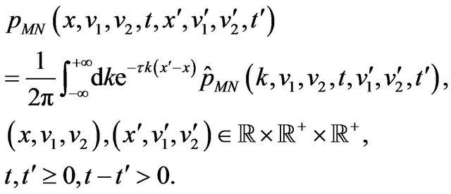
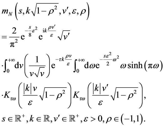
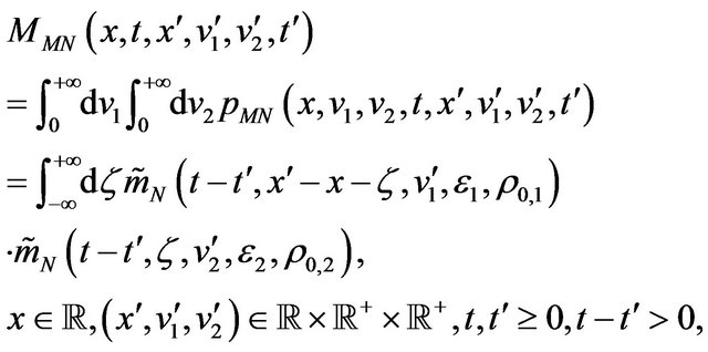
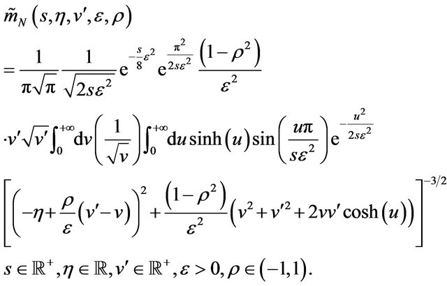
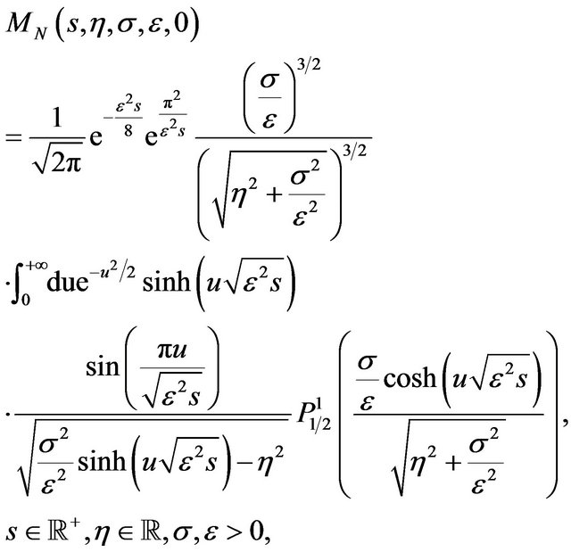
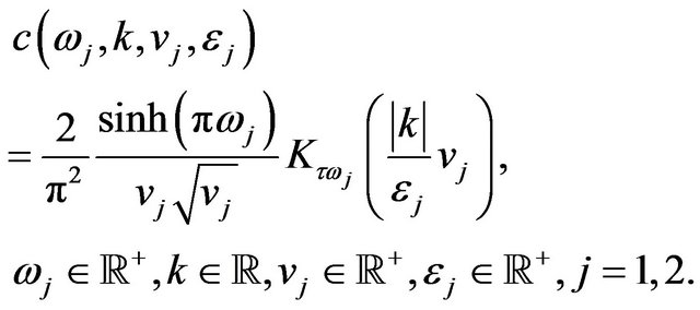
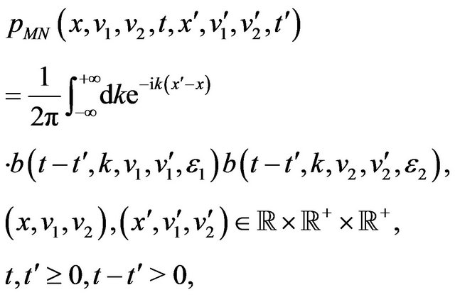
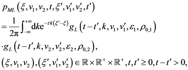
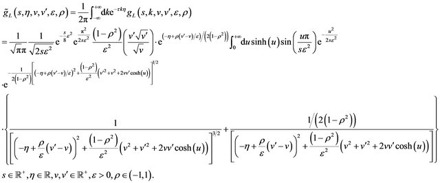
The main result of this Section is the following formula:
 (27)
(27)
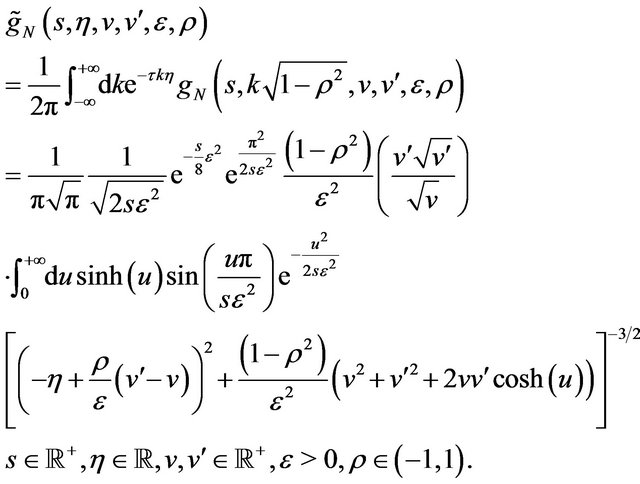
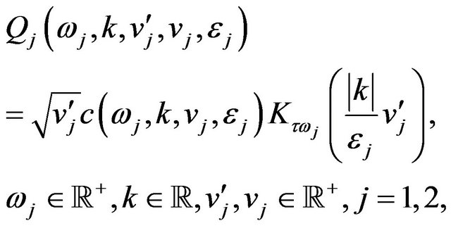
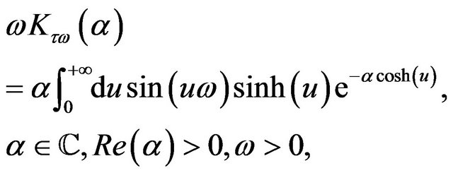
where τ is the imaginary unit and the function  is the “heat kernel for the Kontorovich-Lebedev transform” (see [12] p. 748). That is:
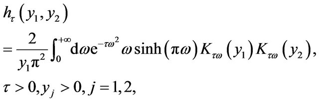 (28)
(28)
where  and
and  denote respectively the hyperbolic sine and the second type modified Bessel function of order
  (see [15] p. 5). With a simple change of variables Formula (27) can be rewritten as follows:
 (29)
(29)
where
 (30)
(30)
Let  be the Fourier transform of
  with respect to the
  variable, we have:
 (31)
(31)
Using (29), (31) and the properties of the Fourier transform we have:
 (32)
(32)
where  is the Fourier transform of
  with respect to the
  variable, that is:
(33)
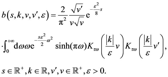
Note that Formula (27) and similarly Formulae (29), (32) give the transition probability density function  as a one dimensional Fourier integral of a known integrand. The integrand has a special form, in fact it contains the product of two copies of a function evaluated in two different points. This function, defined in (30) or in (33), is a one dimensional integral of an explicitly known integrand. That is Formulae (27), (29), (32) are three dimensional integrals. However the special form of their integrands mentioned above implies that the evaluation of these three dimensional integrals with an elementary quadrature rule can be done at the computational cost of a two dimensional integral.
Note that the function  defined in (33) when
 ,
,  ,
,  and
and  is the transition probability density function of the normal SABR model. This can be seen proceeding as done at the end of this Section to deduce (27) or simply verifying that
  satisfies the Fokker Planck equation associated to (13), (14) when
  with the appropriate initial and boundary conditions.
Formula (33) for the transition probability density function of the normal SABR model is a new and useful formula that can substitute the formula commonly used in the mathematical finance literature, that is Formula (120) of [9], that is based on the McKean formula for the heat kernel of the Poincaré plane. The integral that appears in (33) is a one dimensional integral of a smooth function whose numerical evaluation is easier than the evaluation of the integral of a singular function contained in Formula (120) of [9]. Moreover Formulae (27) and (33) are deduced using elementary tools, that is: the Fourier transform, the method of separation of variables and the results of [12] on the Kontorovich Lebedev transform. The McKean formula is derived using the differential geometry of the Poincaré plane. That is Formula (33) and its elementary derivation simplify the study of the normal SABR model.
Formula (27) can be used to deduce some useful consequences. For example from Formula (27) it is possible to deduce an explicit formula for the marginal probability distribution  of the forward prices/rates stochastic process defined by (18)-(23) under the assumptions (4)- (9), that is:
 (34)
(34)
where  is given by:
 (35)
(35)
The function  can be rewritten as follows:
 (36)
(36)
where  is given by:
 (37)
(37)
An alternative expression of the marginal probability distribution (34) can be obtained using Formula (32), that is:
 (38)
(38)
where  is given by:
(39)
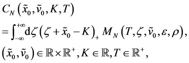
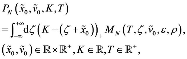
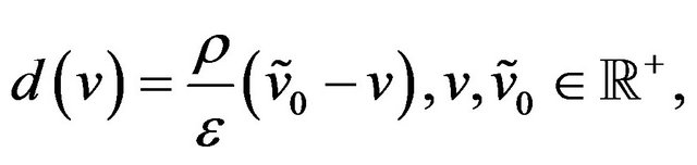
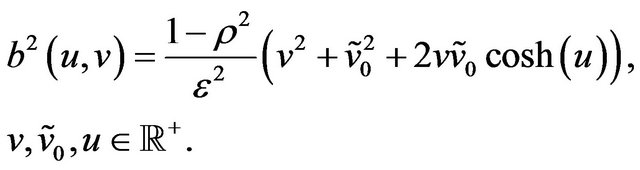
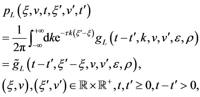
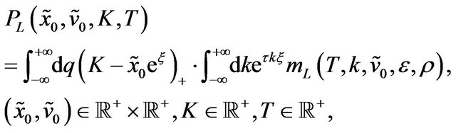
From (27) using the no arbitrage pricing theory formulae to price in the normal multiscale SABR model European call and put options can be derived. The assumption that the risk free interest rate is deterministic during the life time of the priced option implies that the forward prices/rates coincide with the futures prices/rates. In fact the forward price is a martingale under the (forward) measure associated to (18)-(23) and the futures price is a martingale under the risk-neutral measure. However if the risk free interest rate is deterministic the forward measure and the risk neutral measure coincide (see [13], Proposition 3.1). Hence we can assume that we are working with futures prices/rates instead of with forward prices/rates and we can exploit the fact that these prices/rates are martingales under the risk-neutral measure. That is the risk neutral measure used to compute the option prices and the “physical” measure used to describe the underlying dynamics defined by (18)-(23) are the same (see [13], Proposition 3.1).
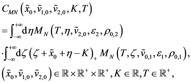
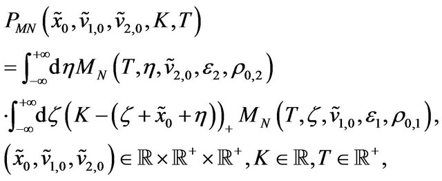
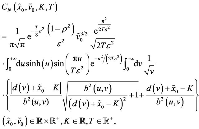
Under the previous assumption on the risk free interest rate manipulating Formulae (27), (34) and using the results contained in [12] we obtain formulae to price European call and put options in the normal multiscale SABR model. That is the formulae for the prices  and
and  at time
  of respectively European call and put options with strike price
  and maturity time
  (i.e. time to maturity
  since
since  is assumed to be “today”) when the forward price of the underlying and the values of the stochastic volatilities at time
  (that is today) are respectively
 ,
,  ,
,  are:
are:
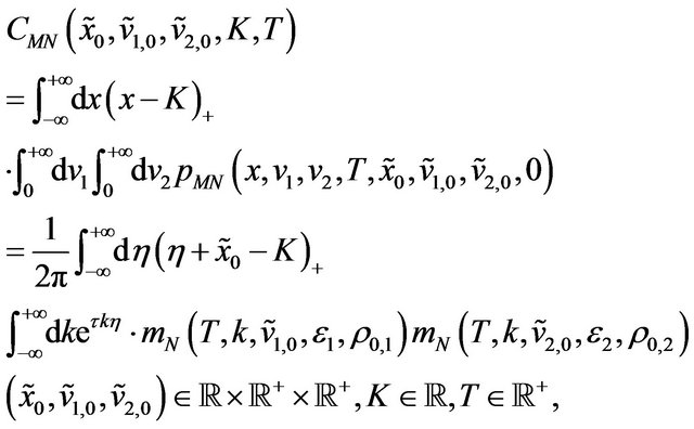 (40)
(40)
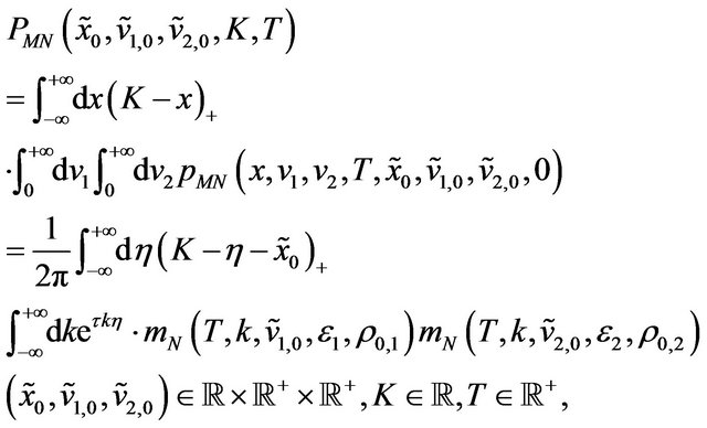 (41)
(41)
where .
.
Note that since in the normal multiscale SABR model the forward prices/rates can be negative we have chosen  instead of
  as it is done when models with positive asset prices are considered. Moreover in (40), (41) we have chosen the discount factor equal to one, that is we have chosen the risk free interest rate equal to zero. This choice is due to the desire of keeping the expression of Formulae (40), (41) simple and can be easily removed.
Formulae (40), (41) can be rewritten as follows:
 (42)
(42)
 (43)
(43)
where  is given by:
 (44)
(44)
when  Formula (44) reduces to:
 (45)
(45)
where  is the Legendre function of the first kind of parameters
 ,
,  (see [15] p. 180). From (45) it follows that Formulae (40), (41) can be simplified when
 .
.
In the case of the normal SABR model Formulae (40) and (41) reduce respectively to the following formulae:
 (46)
(46)
 (47)
(47)
where  is the stochastic volatility at time
  (see (17)). Moreover in (46) the integral with respect to the
  variable can be computed explicitly, we have:
(48)
where
 (49)
(49)
A formula analogous to (48) can be obtained for the put option price  integrating (47) with respect to the
  variable.
Note that also the integrals in the  variable appearing in Formulae (40) and (41) can be done explicitly. However in the case of Formulae (40) and (41) this integration leads to formulae computationally useless. In fact in Formulae (40) and (41) the evaluation of the functions
  in a point of the
  grid implies the computation of a two dimensional integral, however these function are independent of
 ,
,  and
and , the value of these functions on a grid in the
  variable can be computed out of the
 ,
,  ,
,  loops. Note that the double integral coming from the integration with respect to the
  variable couples
 ,
,  and
and  variables.
In Formulae (46)-(48) for simplicity the discount factor has been chosen equal to one. This assumption can be easily removed.
Let us derive Formula (27). The reader not interested in this derivation can move to Section 3. We begin deducing Formula (27) when . Under the assumptions (4)-(9), when
 let us consider the backward Kolmogorov equation associated to the stochastic differential Equations (18)-(20) satisfied by the function
  as a function of the variables
 , we have:
 (50)
(50)
Equation (50) must be equipped with an initial condition in , that is:
 (51)
(51)
and appropriate boundary conditions.
Let  be the conjugate variable in the Fourier transform of the
  variable, it is easy to see that the Fourier transform
  of
of  with respect to
  is the solution of the following problem:
 (52)
(52)
with the initial condition:
 (53)
(53)
and the appropriate boundary conditions. To solve Problem (52) and (53), we proceed by separation of variables, that is we assume:
 (54)
(54)
where ,
,  , are functions to be determined. Substituting (54) in (52) we have:
 (55)
(55)
That is the assumption (54) reduces the solution of (52) and (53) to the solution of the following initial value problems:
 (56)
(56)
 (57)
(57)
with the appropriate boundary conditions. The constant  appearing in (56) comes from the separation of variables.
To solve problems (56) and (57) we assume that the functions ,
,  , have the following form:
 (58)
(58)
 (59)
(59)
where ,
,  , are functions to be determined. Note that for
  the function
  depends on
 , however the product
  does not depend on
 . Equations (58) and (59) imply that Equation (56) reduce to the following linear ordinary differential equations satisfied by
 ,
, :
:
 (60)
(60)
with the boundary condition:
 (61)
(61)
The boundary condition (61) is derived from the boundary conditions imposed to the solution of (50) (and as a consequence to the solution of (56)) and follows from the fact that we are looking for solutions of (56) that are probability density functions. Imposing the boundary condition (61) to the general solution of (60) we have:
 (62)
(62)
where for  the function
  is an “arbitrary constant” of the solution of (60), that is
  is independent of
 , that can be determined through (58), (59) imposing the initial conditions (57) to the parabolic Equation (56). In fact we have:
 (63)
(63)
using the inversion formula of the Kontorovich Lebedev Transform (see Formula (3) of [12] and the references therein) we have:
 (64)
(64)
Using (63) and (64) we obtain the following formula for the function :
:
 (65)
(65)
where
 (66)
(66)
When the boundary conditions are chosen appropriately the solution (65) of the backward Kolmogorov Equation (50) with  in the “past” variables
 ,
,  ,
,  ,
,  with the final condition (51) is the solution of the Fokker Planck Equation (24) with
  (also known as forward Kolmogorov equation) in the “future” variables
 ,
,  ,
,  ,
,  with the initial condition (25). Formula (65) is deduced assuming that
 , when
  replacing in (65),
  ,
,  ,
, respectively with
 ,
,  and
and
 we obtain (27) and it is easy to verify that (27) satisfies the Fokker Planck Equation (24) with initial condition (25) and the appropriate boundary conditions.
Note that the change of variables used to go from the  case to the
 ,
,  case generalizes to the multiscale context the change of variables used in [9] in the study of the normal SABR model to go from the
  case to the
  case. Recall that the McKean formula for the heat kernel of the Poincaré plane gives the transition probability density function of the normal SABR model when
 .
.
Note that (39) can be derived with elementary computations from (30) using the following representation formulae that can be deduced from Formula (46) p. 35 of [16], Formula (9) p. 176 of [17], and Formula (1.1) of [18]:
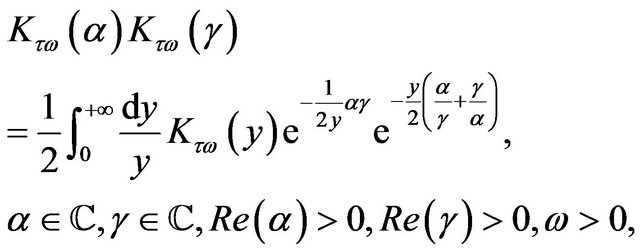 (67)
(67)
 (68)
(68)
where  denotes the set of the complex numbers and
  denotes the real part of the complex number z. Formulae (67) and (68) generalize to complex arguments respectively Formula (15), p. 747 of [12] and Formula (32) p. 99 of [19].
It is easy to see that Formula (33) for the normal SABR model can be deduced proceeding as done to deduce Formula (27) for the normal multiscale SABR model.
3. The Lognormal SABR and Multiscale SABR Models
Let us consider the lognormal multiscale SABR model, those are Models (1)-(3) when , we have:
 (69)
(69)
 (70)
(70)
 (71)
(71)
with the initial conditions:
 (72)
(72)
 (73)
(73)
 (74)
(74)
where, as already said,  ,
,  ,
,  , are random variables that we assume to be concentrated in a point with probability one. To the assumption
 ,
,  , done previously we add the assumption
 . Moreover we assume that the quantities
 ,
,  , are positive constants such that
  and that the conditions (4)-(9) hold. Recall that when
  is positive with probability one it follows that
  solution of (69)-(74) is positive with probability one for
 . We can conclude that when
  with probability one the absolute value in (69) can be dropped.
Let us derive a formula for the transition probability density function of the stochastic process defined implicitly by (69)-(74).
Let  be a constant such that
  is positive with probability one, we define the variable
 ,
, . Using the variable
 ,
,  , the stochastic differential Equations (69)-(71) for
  can be rewritten as follows:
 (75)
(75)
 (76)
(76)
 (77)
(77)
Let us choose  the previous change of variables transforms the Equations (69)-(71) into the Equations (75)-(77) for
  and the initial conditions (72)-(74) into the initial conditions:
 (78)
(78)
 (79)
(79)
 (80)
(80)
The variable ,
,  , is called log-return of the forward prices/rates. Note that the differential Equation (75) in the log return variable
 ,
,  , of the lognormal multiscale SABR model differs from the corresponding equation (18) in the forward prices/rates variable
 ,
,  , of the normal multiscale SABR model only for the presence of the drift term
that appears in (75) and is absent in (18). For this reason under the previous assumptions it is possible to derive a formula for the transition probability density function  associated to the process
 ,
,  , implicitly defined by (75)-(77) when
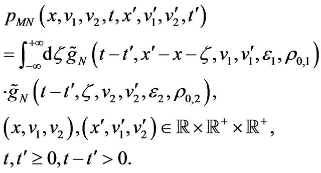
  with the initial conditions (78)-(80) arguing as done in Section 2 to study the normal multiscale SABR model. Proceeding in this way we obtain the following formula:
 (81)
(81)
where ,
,  ,
,  ,
,  ,
,  , and the remaining notation is the one used in Section 2. The function
  is given by:
 (82)
(82)
where
 (83)
(83)
Note that when  in (81) we must choose
 ,
,  ,
, . From (81) and the properties of the Fourier transform we have:
 (84)
(84)
where  is the Fourier transform with respect to the
  variable of
  and
and  is the conjugate variable in the Fourier transform of the
  variable. Using Formulae (67) and (68) an elementary computation gives:
(85)
Note that Formula (81) gives the transition probability density function  of the lognormal multiscale SABR model using the log-return of the forward prices/rates variable, that is:
 (86)
(86)
where we assume ,
,  ,
,  ,
,  ,
,  ,
, . Note that when
  we must choose
 ,
, . Note that Formula (86) holds when
 . This (closed form) formula when
  is a new formula, in fact up to now when
  only series expansions in powers of
  with base point
  have been known for
  (see, for example, [10], [11] and the references therein).
Note that the lognormal SABR model is a special case of the Hull and White stochastic volatility model. It is easy to see that the analysis presented here for the lognormal SABR model can be extended to the study of the Hull and White model in presence of a nonzero correlation coefficient between the stochastic differentials of the Wiener processes of the model. In this way it is possible to obtain new (closed form) formulae for the transition probability density function of the Hull and White model and for the corresponding European call and put option prices. These formulae will be presented elsewhere.
The previous formulae for the transition probability density functions  and
and  written using the logreturn variable
 ,
,  , can be easily rewritten in the original forward prices/rates variable
 ,
, .
.
Finally starting from (84) and proceeding as done in Section 2 we obtain the following formulae for the prices  and
and  in the lognormal multiscale SABR model at time
  of respectively European call and put options with strike price
 , maturity time
  when the price of the underlying and the values of the stochastic volatilities at time
  (that is today) are given respectively by
 ,
,  ,
, :
:
(87)
(88)
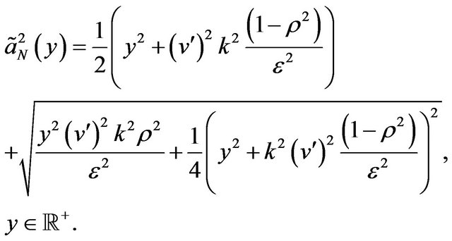
where the function  is given by:
(89)
and ,
,  , is given by (83). Formula (89) can be rewritten as follows:
 (90)
(90)
where  is given by:
 (91)
(91)
The numerical experience presented in Section 5 has shown that in the evaluation of Formula (90) the complex square root that defines  must be computed very accurately. For this purpose in the numerical experiments we have found useful to exploit the results of [20].
Note that the integrands of the integrals appearing in Formulae (87) and (88) have the same special form of the integrands of Formulae (40) and (41). This implies that evaluating Formulae (87) and (88) has the same computational cost than evaluating Formulae (40) and (41). This last cost has been discussed in Section 2.
In the case of the lognormal SABR model Formulae (87) and (88) reduce respectively to the following formulae:
 (92)
(92)
 (93)
(93)
where ,
,  are respectively the prices at time
  of European call and put options in the lognormal SABR model when the initial conditions (16) and (17) hold and
  is given by (90). In the option pricing formulae (87), (88), (92), (93) the risk free interest rate has been chosen equal to zero and as a consequence the discount factor has been chosen equal to one. This choice is made to simplify the formulae and can be removed easily.
4. A Calibration Problem for the Normal and Lognormal SABR and Multiscale SABR Models
Let  be a positive integer and
  be the
  - dimensional real Euclidean space. We formulate a calibration problem for the models studied in Section 2 and 3.
Under the assumptions (4)-(9) the normal and lognormal multiscale SABR models (18)-(20) and (69)-(71) together with the associated option pricing Formulae (40), (41) and (87), (88) are parameterized by six real quantities, that is: the parameters ,
,  , the correlation coefficients
 ,
,  , and the initial stochastic volatilities
 ,
, . These quantities are the unknowns that must be determined in the calibration problem. In this Section and in the numerical experiments presented in Section 5 we consider as a parameter that must be determined in the calibration problem also the risk free interest rate
 . The risk free interest rate
  appears in the option pricing formulae when we consider the discount factor that, for simplicity, has been omitted in Formulae (40), (41), (87), (88). That is all together when we consider the normal and lognormal multiscale SABR models there are seven real parameters that must be determined in the calibration problem. We introduce the vector
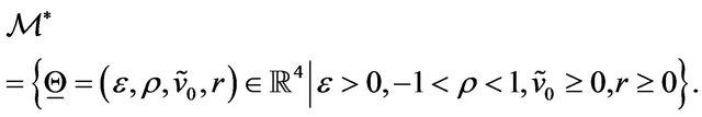
  and the set
  defined as follows:
 (94)
(94)
In the calibration problem for the (normal and lognormal) multiscale SABR models the vector  is the unknown that must be determined and
  defines the set of the “feasible” vectors of the calibration problem. That is
  is the set of vectors that satisfy the “physical” constraints that follow from the meaning of the parameters in the model equations.
Similarly when we consider the (normal and lognormal) SABR models the unknown of the calibration problem is the vector  and the set
  of the “feasible” vectors of the calibration problem is defined as follows:
(95)
To keep the notation simple in the formulation of the calibration problems for the SABR and multiscale SABR models we denote with the same symbol  a vector belonging to
  or to
or to .
.
The calibration problems considered use as data a set of option prices observed at a given observation time. The option price data are fitted in the least squares sense with the option pricing formulae deduced in Sections 2 and 3 (completed with the discount factors) imposing the constraints defined in (94) or (95). That is the calibration problem is formulated as a nonlinear constrained least squares problem.
Let ,
,  be positive integers,
  be the observation time and
  be the forward prices/rates observed at time
 . Let
. Let ,
,
 ,
,  ,
,  , be respectively the observed prices at time
  of the European call options having maturity time
  and strike price
 ,
,  , and of the European put options having maturity time
  and strike price
 ,
, . Note that the values
 ,
,  ,
,  , and
, and ,
,  ,
,  , are not necessarily distinct. For example options having the same maturity time and several strike prices can be considered, in this case in the previous sets some of the maturity times are repeated. Moreover let
  and let
 ,
,  ,
,
 ,
,  ,
,  ,
,
 , be the prices as a function of
  of the European call and put options obtained evaluating, respectively, Formulae (40), (41) and (87), (88) completed with the discount factors when
  (i.e. the maturity time),
  , or
, or ,
,  , and
, and . Note that when
  Formulae (40), (41) and (87), (88) give the option prices at time
  and that we are computing the prices at time
 . Some obvious changes in the interpretation of the formulae derived in Sections 2 and 3 are necessary to handle this situation. For example the initial stochastic volatilities
 ,
,  that in (40), (41) and (87), (88) denote the volatilities at time
  must be interpreted as the volatilities at time
 . Similarly when the SABR models are considered let
 ,
,  ,
,  ,
,  ,
,
 ,
,  , be the corresponding prices of the European call and put options obtained using Formulae (40), (41) and (87), (88) completed with the discount factors. Note that when we consider
 ,
, ,
,  ,
,  , and
, and ,
,  ,
,  ,
,  , the vector
  is a vector belonging to
 . In general
  and
and  are functions of the observation time
 , however, to simplify the notation, we omit this dependence. For notational convenience we define the following sets
 ,
, .
.
The calibration problem considered is formulated as follows:
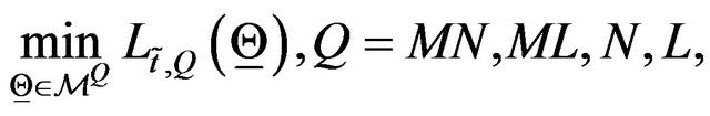 (96)
(96)
where the objective function  is given by:
 (97)
(97)
Problem (96) is a nonlinear constrained least squares problem. Note that when in (97) we choose  or
or  we calibrate respectively the normal and lognormal multiscale SABR model and when we choose
  or
or  we calibrate respectively the normal and lognormal SABR model. The solution of the calibration problem is the vector
  that solves problem (96). Problem (96) is only a formulation of the calibration problem between many other possible formulations.
In the numerical experiments presented in Section 5 Problem (96) is solved with a local minimization method that is explained below. For  we choose the initial guess of the minimization procedure used to solve Problem (96) exploring the feasible region
 . This is done taking a set of random points belonging to
  and evaluating the objective function on this set of points. The initial guess of the minimization method is chosen among these points using a heuristic rule. The minimization method used is a variable metric steepest descent method (see [21]). This method is an iterative procedure that, given an initial vector
  , generates a sequence
 ,
,  , of vectors,
  ,
,  , obtained making a step in the direction of minus the gradient with respect to
  of
of  computed in a suitable metric that depends on the constraints defined in
 . The procedure stops when the following criterion is satisfied:
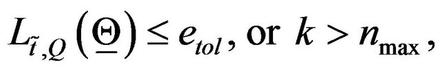 (98)
(98)
where ,
,  are given positive constants. Details of the implementation of the variable metric steepest descent method used to solve the calibration problem can be found in [6].
5. Some Numerical Experiments Using Real Data
In the numerical experiments presented in this Section the option prices computed evaluating with numerical quadratures the integrals contained in Formulae (40), (41), (46), (47), (87), (88), (92), (93) and completing the results obtained with the appropriate discount factors are compared with the option prices actually observed. The numerical quadratures are performed using the composite midpoint quadrature rule with 1000 nodes in each coordinate direction. These choices guarantee approximately six significant digits correct in the option prices.
We present two numerical experiments based on the calibration problem of Section 4. The stopping parameters of the minimization algorithm introduced in (98) have been chosen as follows: ,
,  .
.
In the first experiment we consider the daily values of the futures price on the EUR/USD currency’s exchange rate having maturity September 16th, 2011, (the third Friday of September 2011) and the daily prices of the corresponding European call and put options with expiry date September 9th, 2011 and strike prices  ,
, . The strike prices
 ,
,  , are expressed in USD. These prices are observed in the time period that goes from September 27th, 2010, to July 19th, 2011. The observations are made daily and the prices considered are the closing prices of the day. Recall that a year is made of about 250 - 260 trading days and a month is made of about 21 trading days. Figure 1 shows the futures price EUR/USD (ticker YTU1 Curncy) (blue line) and the EUR/USD currency’s exchange rate (pink line) as a function of time. Figures 2 and 3 show respectively the prices (in USD) of the corresponding call and put options with maturity time September 9th, 2011 and strike price
 ,
,  , as a function of time.
The computation of thirty-six option prices using the midpoint quadrature rule as specified previously requires three and half seconds on the Intel CORE Duo CPU T6400 2 GHz processor.
In the first experiment we use the normal SABR and multiscale SABR models to interpret these data. In par-

Figure 1. YTU1 (blue line) and EUR/USD currency’s exchange rate (pink line) versus time.
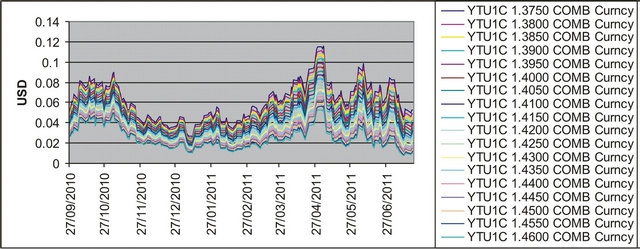
Figure 2. Call option prices on YTU1 with strike price ,
,  , and expiry date T = September 9th, 2011 versus time.
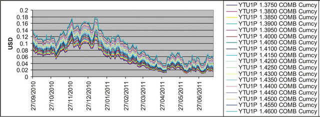
Figure 3. Put option prices on YTU1 with strike price ,
,  , and expiry date T = September 9th, 2011 versus time.
ticular for these models we solve the calibration problem posed in Section 4. We solve Problem (96) when ,
,  and
and  for
for ,
,  , where
 ,
,  , using as data the futures prices (YTU1 ticker of Figure 1) and the prices of the previously mentioned eighteen call and eighteen put options available at
 ,
,  , (Figures 2 and 3). The choice of the dates
 ,
,  , exploits the fact that the formulae deduced in Sections 2 and 3 are closed form formulae that have no limitations. In particular they can be used when the products
 ,
,  ,
,  , are not small. This is the case when we consider the dates chosen previously. Recall that the option pricing formulae for the SABR models contained in [1], [9] are asymptotic formulae that hold when
  is small.
Tables 1 and 2 show respectively the parameter values obtained as solution of the calibration problems (96) for the normal SABR and multiscale SABR models when we consider the data relative to ,
, .
.
The calibrated models, that is those with the parameter values given in Tables 1 and 2, are used to forecast option prices one day ahead of the current date, that is ahead of the observation day of the prices used to calibrate the model. The forecasts are made evaluating formulae (40) and (41) when  and evaluating formulae (46) and (47) when
  multiplied by the appropriate discount factors. These formulae are evaluated using as futures price the futures price observed the day of the forecast. The volatilities
  and
and  obtained from the calibration problem are taken as proxies of the volatilities the day of the forecast.
Let us define the moneyness of an option a given day as the ratio between the strike price of the option and the futures price on the EUR/USD exchange rate of that day. Figures 4 and 5 show the forecast option prices one day in the future (i.e. at time  with
with  equal one day) the observed option prices and the relative errors of
Table 1. Solution of the calibration problem: Normal SABR model (FX experiment).
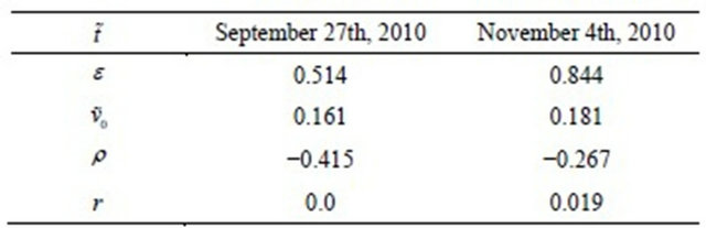
Table 2. Solution of the calibration problem: Normal multiscale SABR model (FX experiment).

the forecast option prices one day in the future compared with the observed prices as a function of the moneyness of the day of the forecast (i.e. ). We consider the relative error obtained using the normal SABR model (Figures 4(a) and 5(a)) and the normal multiscale SABR model (Figures 4(b) and 5(b)) calibrated using the option prices of
  (Figure 4), and
  (Figure 5). The futures prices used in the forecasts are
  and
and  where
where  .
.
Figures 4 and 5 show that in this experiment the normal multiscale SABR model outperforms the normal SABR model. This is probably due to the fact that the use of two volatilities in the multiscale SABR model captures efficiently the “smile” effect contained in the option prices. In fact the values of the constants  and
and  resulting from the solution of the calibration problem
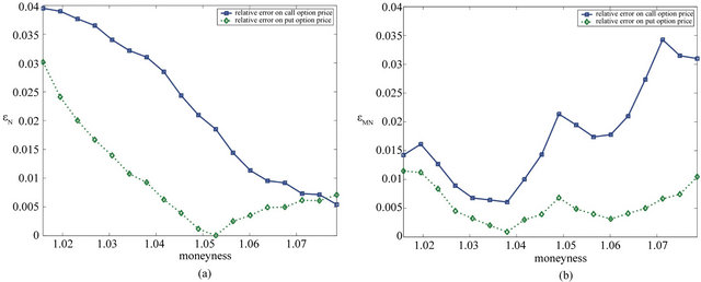
Figure 4. Relative errors obtained using the normal SABR (a) and multiscale SABR (b) models calibrated at  September 27th, 2010 versus moneyness (FX experiment).

Figure 5. Relative errors obtained using the normal SABR (a) and multiscale SABR (b) models calibrated at  November 4th, 2010 versus moneyness (FX experiment).
shown in Table 2 differ approximately of a factor two showing that the presence of the second volatility is really useful to interpret the data. Note that the values of  and
and  shown in Table 2 do not differ of one or more orders of magnitude as found for similar constants in previous studies [6,7]. In [6] and [7] a multiscale Heston model has been used to study electric power prices. Electric power prices show severe spikes and abrupt changes that justify the huge difference in the
 ,
,  values (two orders of magnitude) while the futures price of EUR/USD currency’s exchange rate is a much more well behaved quantity. However also the factor two that separates approximately the values of
  and
and  shown in Table 2 corresponds to a relevant difference in the forecasting ability of the normal SABR and multiscale SABR models as shown in Figures 4 and 5.
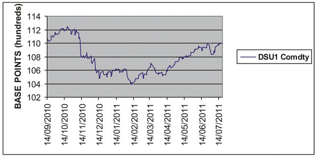
In the second experiment we consider the daily observed values of the USA five-year interest rate swap (see Figure 6(a)), the corresponding futures prices having maturity September 30th, 2011 (the ticker DSU1 in Figure 6(b)) and the prices of the corresponding European call and put options with expiry date September 19th, 2011 and strike prices
 ,
, . These prices are observed in the period going from September 14th, 2010, to July 20th, 2011. The strike prices
 ,
,  , are expressed in hundreds of base points that is, for example,
  corresponds to an interest rate 106 −
 (a)
(a)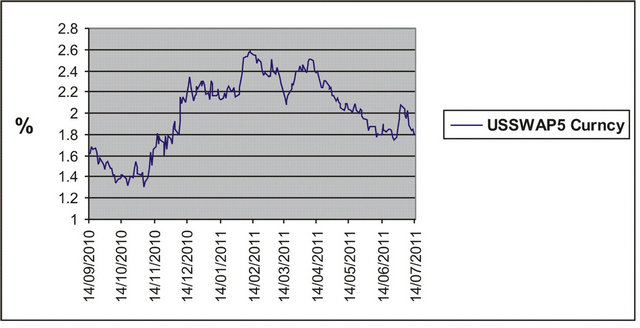 (b)
(b)
Figure 6. Observed USA five-year interest rate swap (a) and the corresponding futures price DSU1 having maturity September, 2011 (b) versus time.
100 = 6 that is 600 base points, this corresponds to an interest rate of  per year (see Figures 7 and 8).
We consider two dates  and
and , where the values of the corresponding futures prices (ticker DSU1 Figure 6(b)) are
  and
and . That is we consider two dates the first one
  selected in a period where the oscillations of the futures price are small and the second one
  selected at the beginning of the fall of the futures price (see Figure 6(b)). Note that from November 12th, 2010 to December 15th, 2010 the futures price goes from the value of 110 to the value of 104. Recall that these futures prices are expressed in hundreds of base points.
Tables 3 and 4 show the parameter values obtained calibrating the lognormal SABR and multiscale SABR models on the data discussed above relative to the USA five-year interest rate swap futures price and its options observed at ,
, . In particular Table 4 shows that the values of the parameters
  and
and  of the lognormal multiscale model resulting from the calibration differ of approximately a factor two.
Figures 9(a), 10(a), 11(a) and 12(a) show the observed option prices and the forecast option prices as a function of the moneyness at the date  (Figures 9(a) and 10(a)) and
  (Figures 11(a) and 12(a)). The forecast option prices are obtained using the lognormal SABR model (see Figures 9(a) and 11(a)) and the multiscale SABR models (see Figures 10(a) and 12(a)).
Figures 9(b), 10(b), 11(b) and 12(b) show the the relative errors committed on the forecast option prices one day ahead of the current day as a function of the moneyness. In particular we use the values of the model parameters obtained calibrating the model using the data at  to forecast the option prices at
  (see Figures 9 and 10), and the values of the parameters obtained calibrating the model using the data at
  to forecast the option prices at
  (see Figures 11 and 12), where
 .
.
Figures 9(b), 10(b), 11(b) and 12(b) show that the use of
Table 3. Solution of the calibration problem: Lognormal SABR model (interest rate swap experiment).

Table 4. Solution of the calibration problem: Lognormal multiscale SABR model (interest rate swap experiment).
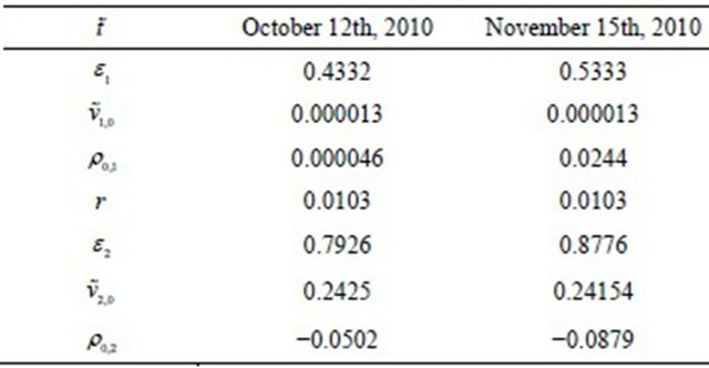
the lognormal multiscale SABR model really improves the results of the forecasting experiment in comparison with the results obtained with the lognormal SABR model. In fact the relative errors on the forecast option prices of the multiscale SABR model (see Figures 10(b) and 12(b)) are smaller than the corresponding relative errors of the SABR model (see Figures 9(b) and 11(b)). In particular the lognormal multiscale SABR model improves substantially the lognormal SABR model in the forecasting of the prices of at the money options (see Figures 9(b), 10(b) and 11(b), 12(b)).
This numerical experiment shows that the use of two volatilities is justified when the forward/futures prices present significant changes in their behaviour. Note that the calibration done using the data of October 12th, 2010 (see Table 4), that is a date before the beginning of the futures price fall, already provides two volatilities of volatilities significantly different (i.e. ) and
) and

Figure 7. Call option prices on DSU1 with strike price ,
,  , and expiry date T = September 19th, 2011 versus time.
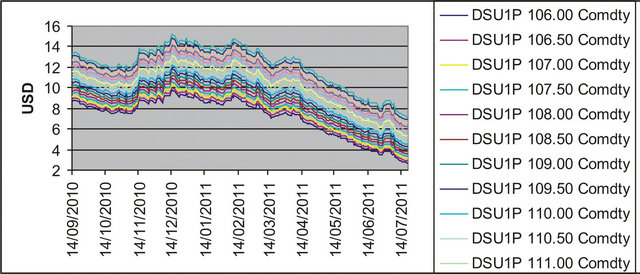
Figure 8. Put option prices on DSU1 with strike price ,
,  , and expiry date T = September 19th, 2011 versus time.
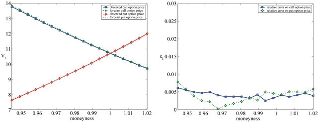 (a) (b)
Figure 9. Observed and forecast prices one day in the future of call and put options (a) and relative errors (b) obtained using the lognormal SABR model calibrated at  versus moneyness (interest rate swap experiment).
this remains true for the parameter values obtained with the data of November 15th, 2010 (see Table 4). However we observe that on November 15th, 2010 the calibration provides values of  and
and  greater than the values provided on October 12th, 2010.
Finally we calibrate the lognormal models every day for approximately two months, that is we calibrate the models in the period going from September 14th, 2010 to November 15th, 2010. The parameter values obtained in the calibration of the lognormal models are shown in
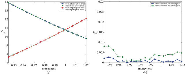
Figure 10. Observed and forecast prices one day in the future of call and put options (a) and relative errors (b) obtained using the lognormal multiscale SABR model calibrated at  versus moneyness (interest rate swap experiment).
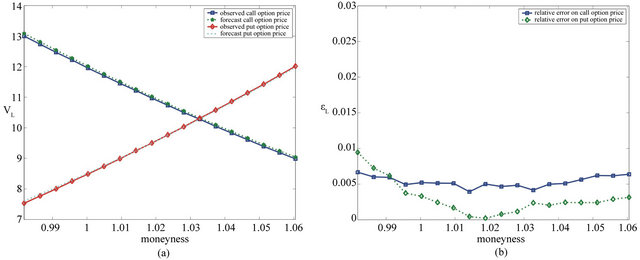
Figure 11. Observed and forecast prices one day in the future of call and put options (a) and relative errors (b) obtained using the lognormal SABR model calibrated at  versus moneyness (interest rate swap experiment).
Figure 13. We can see that the values of the parameters remain substantially unchanged in the two months period except for the values of the parameters  and
and  that show a significant change at the end of October 2010 and during the first fifteen days of November 2010. This is probably due to the deep fall in the futures price in the same period (see Figure 6). This experiment suggests that the lognormal models really interpret the data, in fact the values of the parameters found depend on the dynamics of the futures price and the presence of a significant changes in the values of the volatilities of volatilities
 ,
,  ,
,  may imply abrupt changes in the forward prices/rates variable. Finally Figure 14 shows the relative errors on the forecast option prices one day ahead of the current day obtained using the parameter values shown in Figure 13. We can see that the lognormal multiscale SABR model gives more accurate forecast option prices than the lognormal SABR model. The average and the worst case of the relative errors are respectively 0.0037, 0.028 for the lognormal SABR model and 0.0025, 0.025 for the multiscale SABR model. That is as shown in Figures 9-12 the lognormal multiscale SABR model improves substantially the lognormal SABR model especially in forecasting option prices and in particular prices of at the money options.
6. Conclusion
The closed form formulae for the transition probability
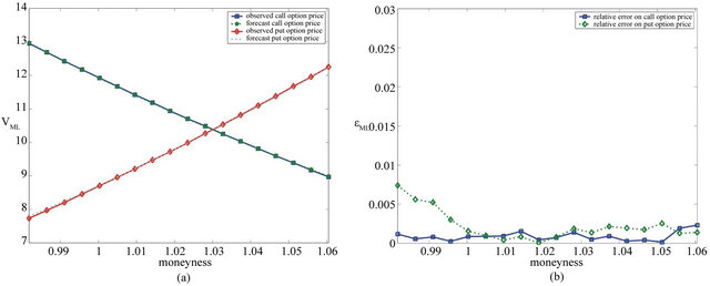
Figure 12. Observed and forecast prices one day in the future of call and put options (a) and relative errors (b) obtained using the lognormal multiscale SABR model calibrated at  versus moneyness (interest rate swap experiment).

Figure 13. Parameter values obtained calibrating the lognormal SABR and multiscale SABR models every day for two months in the period going from September 14th, 2010 to November 15th, 2010 versus time (interest rate swap experiment).
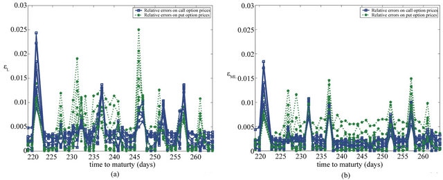
Figure 14. Relative errors on the forecast prices one day in the future of call and put options obtained using lognormal SABR model (a) and lognormal multiscale SABR model; (b) versus time to maturity expressed in days. The period considered goes from September 14th, 2010, to November 15th, 2010 (interest rate swap experiment).
density function of the normal and lognormal SABR and multiscale SABR models derived in this paper are a practical tool to price derivatives on forward prices and rates. In fact using these formulae “easy to use” formulae for the price of European options on futures prices/rates have been deduced and have been used to study the prices of European call and put options on the Eurodollar futures price and on the USA five year interest rate swap futures price. Using these option pricing formulae a calibration problem based on the least squares method is formulated and solved numerically. The models are used to study real data time series. The numerical experiments compare the performance of the SABR and multiscale SABR models in forecasting option prices. The comparison suggests that in the circumstances studied in Section 5 the lognormal SABR model outperforms the normal SABR model and the SABR multiscale models outperform the corresponding SABR models. In general we could say that the multiscale SABR models outperform the corresponding SABR models when the change in time of the data interpreted by the models is sufficiently big. Finally let us point out that the potential of the technique used to derive these formulae can be exploited in other circumstances. In fact the idea of expressing the transition probability density function of a two factor volatility model as a kind of convolution of two copies of the kernel of the corresponding one factor volatility model can be exploited to study the multiscale generalization of other stochastic volatility models. Moreover the closed form formulae for the transition probability density functions of the normal and lognormal SABR and multiscale SABR models presented in this paper deserve further investigation and can be exploited, for example, to price exotic derivatives or to solve new calibration problems.
REFERENCES
- P. S. Hagan, D. Kumar, A. S. Lesniewski and D. E. Woodward, “Managing Smile Risk,” Wilmott Magazine, September 2002, pp. 84-108. http://www.wilmott.com/pdfs/021118-smile.eps
- G. Fiorentini, A. Leon and G. Rubio, “Estimation and Empirical Performance of Heston’s Stochastic Volatility Model: The Case of Thinly Traded Market,” Journal of Empirical Finance, Vol. 9, No. 2, 2002, pp. 225-255. doi:10.1016/S0927-5398(01)00052-4
- B. Chen, C. W. Oosterlee and S. van Weeren, “Analytical Approximation to Constant Maturity Swap Convexity Corrections in a Multi-Factor SABR Model,” International Journal of Theoretical and Applied Finance, Vol 13, No. 7, 2010, pp. 1019-1046. doi:10.1142/S0219024910006091
- F. Mercurio and N. Moreni, “Inflation Modelling with SABR Dynamics,” Risk Magazine, 1 June 2009, pp. 106- 111.
- L. Fatone, F. Mariani, M. C. Recchioni and F. Zirilli, “Calibration of a Multiscale Stochastic Volatility Model Using as Data European Option Prices,” Mathematical Methods in Economics and Finance, Vol. 3, No. 1, 2008, pp. 49-61.
- L. Fatone, F. Mariani, M. C. Recchioni and F. Zirilli, “An Explicitly Solvable Multi-Scale Stochastic Volatility Model: Option Pricing and Calibration,” Journal of Futures Markets, Vol. 29, No. 9, 2009, pp. 862-893. doi:10.1002/fut.20390
- L. Fatone, F. Mariani, M. C. Recchioni and F. Zirilli, “The Analysis of Real Data Using a Multiscale Stochastic Volatility Model,” European Financial Management, Vol. 19, No. 1, 2013, pp. 153-179. doi:10.1111/j.1468-036X.2010.00584.x
- O. Islah, “Solving SABR in Exact Form and Unifying It with LIBOR Market Model,” SSRN eLibrary, 2009. http://papers.ssrn.com/sol3/papers.cfm?astract-id=1489428
- P. S. Hagan, A. S. Lesniewski and D. E. Woodward, “Probability Distribution in the SABR Model of Stochastic Volatility,” 2005. http://lesniewski.us/papers/working/ProbDistrForSABR.eps
- J. Hull and A. White, “The Pricing of Options on Assets with Stochastic Volatilities,” The Journal of Finance, Vol. 42, No. 2, 1987, pp. 281-300. doi:10.1111/j.1540-6261.1987.tb02568.x
- B. A. Surya, “Two-Dimensional Hull-White Model for Stochastic Volatility and Its Nonlinear Filtering Estimation,” International Conference on Computational Science, ICCS 2011, Procedia Computer Science, Vol. 4, 2011, pp. 1431- 1440.
- S. B. Yakubovich, “The Heat Kernel and Heisenberg Inequalities Related to the Kontorovich-Lebedev Transform,” Communications on Pure and Applied Analysis, Vol. 10, No. 2, 2011, pp. 745-760. doi:10.3934/cpaa.2011.10.745
- T. Björk and C. Landen, “On the Term Structure of Futures and forward Prices,” In: H. Geman, D. Madan, S. Pliska and T. Vorst, Eds., Mathematical Finance—Bachelier Congress 2000, Springer Verlag, Berlin, 2002, pp. 111-150.
- M. Musiela and M. Rutkowski, “Martingale Methods in Financial Modelling,” Springer-Verlag, Berlin, 2005.
- A. Erdelyi, W. Magnus, F. Oberhettinger and F. G. Tricomi, “Higher Trascendental Functions,” McGraw-Hill Book Company, New York, 1953.
- A. Erdelyi, W. Magnus, F. Oberhettinger and F. G. Tricomi, “Tables of Integral Transforms,” McGraw-Hill Book Company, New York, 1954.
- A. Erdelyi, W. Magnus, F. Oberhettinger and F. Tricomi, “Tables of Integral Transforms,” McGraw-Hill Book Company, New York, 1954.
- R. Szmytkowski and S. Bielski, “Comment on the Orthogonality of the Macdonald Functions of Imaginary Order,” Journal of Mathematical Analysis and Applications, Vol. 365, No. 1, 2010, pp. 195-197. doi:10.1016/j.jmaa.2009.10.035
- S. B. Yakubovich, “Beurling’s Theorems and Inversion Formulas for Certain Index Trasforms,” Opuscula Mathematica, Vol. 29, No. 1, 2009, pp. 93-110.
- S. Rabinowitz, “How to Find the Square Root of a Complex Number,” Mathematics and Informatics Quarterly, Vol. 3, 1993, pp. 54-56.
- A. Mordecai, “Nonlinear Programming: Analysis and Methods,” Dover Publishing, New York, 2003.