ABSTRACT

It follows from the review on classical wave models that the asymmetry of crest and trough is the direct cause for wave drift. Based on this, a new model of Lagrangian form is constructed. Relative to the Gerstner model, its improvement is reflected in the horizontal motion which includes an explicit drift term. On the one hand, the depth-decay factor for the new drift accords well with that of the particle’s horizontal velocity. It is more rational than that of Stokes drift. On the other hand, the new formula needs no Taylor expansion as for Stokes drift and is applicable for the waves with big slopes. In addition, the new formula can also yield a more rational magnitude for the surface drift than that of Stokes.

Keywords:

Wave Model, Stokes Drift, Ocean Surface Wave, Gerstner Wave, Wave Slope, Breaking Criteria

1. Introduction

The drift caused by water wave was firstly studied by George Gabriel Stokes in 1847. His approximate formula based on small-amplitude wave is known as “Stokes drift” nowadays. Is the wave drift caused by the asymmetry of crest and trough? If the answer is true, then not only the nonlinear Stokes wave with finite amplitude but also the Gerstner wave with large amplitude exists wave drift. Thus the doubt “Do we observe Gerstner waves in wave tank experiments?” in [1] can be well answered. This question stimulates us to reconsider the wave mechanism. Our answer is yes and the remodeling process leads to a new formula for the wave drift which differs from that of Stokes.

In order to understand the wave mechanism, there is a necessity for us to review the wave studies. Historically speaking, the study of water wave can be dated back to the year 1687 when Newton did an experiment with U-tube and got the result “the frequency of deep-water waves must be proportional to the inverse of the square root of the wave length”. As reviewed in [2] , the classical wave theories were mainly developed by the scientists from France, Germany and Britain in the eighteenth and early nineteenth centuries. Among all of them, the representative works are given by Airy (1845) for linear wave, Stokes (1847) for nonlinear wave, Gerstner (1802) for trochoid wave and Earnshaw (1847) for solitary wave. After that time, the progresses are under the existing framework and on the wave-breaking investigation [3] , the wind-wave growing mechanism [4] [5] [6] , the wave-spectrum construction [7] [8] together with its applications in numerical ocean-wave forecast [9] [10] .

As for the study which takes Stokes drift as a special topic [11] - [17] , most of them are about the applications of existing formula which was written down by Stokes in 1847. To make remodeling it needs a new approach. Therefore, the present article only concerns the classical results, especially the aspect of wave drift, given by Airy, Stokes and Gerstner. As for the solitary wave on shallow water given by Earnshaw, it is beyond the topic of periodic wave in deep water and is omitted here. The default form of it is the so-called “gravity wave” on the ocean surface.

2. Classical Wave Models and Related Drift Arguments

As the problem concerned, the default model should be the inviscid and incompressible Navier-Stokes equations. But the solving of these equations involves in determining the upper surface boundary condition which is just the wave to look for [18] . This nonlinear characteristic makes the problem insoluble in essence. So, the classical results for surface waves are merely some kind of approximations and the drift formulas only hold within certain limits.

2.1. On the Linear Wave Model

The classical linear wave theory illustrated in nowadays textbooks [19] [20] , mostly follow from that of Airy (1845). Here the Cartesian coordinate system is adopted and only the 2-dimensional case is concerned. The origin is chosen at the equilibrium level (the average height for the crest and trough) with x and z pointing to the propagating direction and upward direction separately.

On the assumption that the amplitude A is infinitely small relative to the wave-length (related to the wave-number k by), that is, the wave steepness satisfies and the upper boundary can be almost seen as a fixed flat surface, there is a linear approximation for the problem. At this time, the surface traveling wave can be conjectured in the simplest trigonometric form:

(2.1)

here and denote the frequency and the time separately. For the deep- water case with irrotational hypothesis on the flow, the solving of the simplified Navier-Stokes equations yields depth-dependent profiles for the wave and pressure:

(2.2)

(2.3)

together with a dispersion relation. Here and are the water density, gravitational acceleration and constant air pressure on the surface. At this time, the horizontal and vertical velocities are

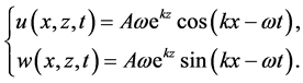(2.4)

According to the web of Wikipedia [21] , the derivation process of the Stokes drift is as follows:

Within the framework of linear theory, the motion distance is very short and the particle’s Lagrangian location can be substituted by the fixed equi- librium in (2.4) which yields the approximations:

(2.5)

Based on this together with Taylor expansion technique, the Stokes drift is then estimated by:

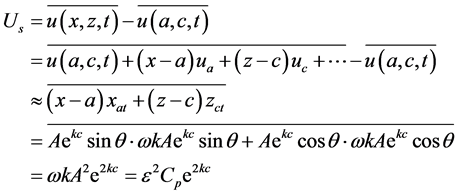(2.6)

with. Here the upper bar and subscripts denote the average and partial derivative calculations separately. is the phase speed of the propagation.

From the above analysis we see the formula for Stokes drift only holds for and the magnitude of it is about at the surface. It is known that, an ideal periodic motion with closed trajectory can not result in a net drift. The generation of Stokes drift should ascribe to the substitution of with. Under the small-amplitude hypothesis it seems reasonable for the approximation. Yet the wave form given by Equation (2.5) can not maintain ideal periodic motion as Equation (2.2) anymore, and its crest and trough have already possessed asymmetric characteristic. As argued in [22] , for a linear wave no particle’s-trajectory is closed, unless the free surface is flat. This implies the shortcoming of the linear model.

2.2. On the Stokes Wave Model

In case is not infinitely small, there is a finite-amplitude wave model owing to Stokes (1847). Notice that accords with the critical case near broken [23] , its application range should be. With the aid of asymptotic expansion technique, the Stokes wave at the surface can be expressed as:

(2.7)

with and [18] [20] . The correspond- ing pressure profile approximates that of linear wave in Equation (2.3).

For this case, the horizontal and vertical velocities are also in the forms of Equation (2.4). But the substitution of with is not suitable anymore. At this time, the estimation of particle’s trajectory is done relative to its initial location. By adopting the substitutions and together with approximating the equations for h and s it results in a Stokes drift [8] which is same as that of linear wave with.

Relative to the linear wave, the Stokes wave looses the range of wave steepness to and it accords well with the actual one which has sharp crests and flat troughs. Its asymmetric characteristic is very distinct.

2.3. On the Gerstner Wave Model

On the assumption that the particle’s trajectory is a circle, Gerstner (1802) found a rotational trochoid wave:

(2.8)

with a dispersion relation. It is an exact solution of the two-dimen- sional Lagrangian equations [20] :

(2.9)

For this case, the water pressure is in a particular form [1] [8] :

(2.10)

which has noting to do with the variables a and t. Here the last term reflect the effect from the fact that the equilibrium is higher than the motionless water level due to the asymmetry of crest and trough. This shows the water pressure is merely in the depth-dependent form provided that the equilibrium is chosen as the reference frame. In fact, to support the t-periodic wave motion the pressure should also vary in a t-periodic manner. In this sense, the reference frame adopted here has defect in describing the particle’s motion, particularly for the drift characteristic. A better choice for the reformation is to take the initial position as a reference.

We note that the Gerstner model (2.8) is actually an alternative form of the approximate linear model (2.5) with a translation on the phase angle by. So the deduction process in Equation (2.6) also holds for small. This indicates the wave drift still exists for Gerstner model from the viewpoint of Taylor expansion. In [1] the net drift observed in wave tank experiments had ever doubted, after all, the particles’s trajectories of a Gerstner wave should be circles. He had improved the model by adopting the viscosity. However, the effect of viscosity to the gravity wave is very small, its contribution to the wave drift should be limited. There should be other deep reasons for this.

In addition, it follows from Equation (2.8) that the particle’s horizontal velocity at the wave crest equals to. Notice that the wave breaks for [23] , the application range of wave steepness for Gerstner model should be. Relative to the Stokes wave, its advantages lie in the concise expression and the abandon of irrotational hypothesis. To some extent, it accords better with the actual one which has sharp crests and flat troughs. Along with the increasing of, the asymmetry of crest and trough becomes serious and for big the Taylor expansion around the equilibrium may result in big error which threaten the feasibility of Stokes drift formula. Hence, there is a necessity for us to remodel the wave drift, particularly in the range.

In addition, it is easy to check that

(2.11)

is also an exact solution to the Lagrangian equations in case a steady flow U exists. However, it follows from [24] that the substitution of steady flow with Stokes drift is not permitted since no steady wave exists of this form.

3. Remodeling the Wave Motion

From the previous analysis we know Airy, Stokes and Gerstner adopted a same approach, that is, to take the conjectured wave forms as the preconditions. What is more, the water pressures are given as corollaries in the last. Here we take an inverse approach to do so. Let the wave model be the object, the conjecture is done on the pressure.

Take one water particle as the research object, we describe it by Lagrangian coordinates with the initial position as the reference. We assume that the small particle possesses a cubic shape and it maintains unchanged during the moving process. Then it follows from [25] that and. At this time, the Equations (2.9) is simplified to

(3.1)

3.1. On the Pressure

For a hydrostatic case with constant density, the water pressure increases linearly along with the water-layer thickness s, that is,. When the fluid has a moving upper surface it may also obey this rule with

(3.2)

this is the so-called “quasi-hydrostatic approximation” adopted in physical oceanography [18] . As the problem concerned, if this kind of approximation is adopted, then it follows from Equation (3.1) that the vertical acceleration. This means the vertical velocity almost keep unchanged. It is impossible! The common sense is that the vertical velocities at the crest and the trough are all zero but those at the mean level are not zero.

There is another case, might as well, call it by “gravitational approximation” which takes the gravity as the main restoring force. For this case, there should be as the particle is on the upper crest part. For this case,. This means there is no relative vertical force between two arbitrary water layers. Hence, the horizontal pressure gradient force due to the slant water body is empty which leads to. This is also a strange case.

In fact, the quasi-hydrostatic and gravitational approximations are two extreme cases: the vertical pressure gradient force is too strong for the first case and too weak for the second case. Notice that the pressure formulas (2.3) and (2.10) for the linear, Stokes and Gerstner waves are deduced from the Navier- Stokes equations and their forms are very objective, we follow them and estimate the pressure by

(3.3)

Here the preconditioned sine or cosine function is substituted by an undetermined free surface. The modification is also reflected in the exponent, use to substitute as in Equation (2.10), which accords well with the dynamic boundary condition at the surface for the case. We note that the incorporating of here is permitted. In fact, under the Lagrangian frame, the functions and can be all expressed by the variables and. Yet, under the Euler frame whose variables are and, it is strange to incorporate into Equation (2.3). As for the effect caused by the height difference between the equilibrium and motionless water level, one can recall it back to improve the model.

3.2. Model Construction

To insert the pressure expression (3.3) into Equations (3.1) it yields

(3.4)

Notice that the wave is a synthesis of transversal and longitudinal waves, with the aid of these two equations we model them separately. To denote

(3.5)

then

with. At this time, the free surface possesses a Lag- rangian description and an Euler description. With the new denotations Equation (3.4) can be further simplified to

(3.6)

These mean the horizontal motion is due to the pressure-gradient force caused by the slant water body and the vertical motion is due to the variation of the surface elevation itself (can be understood as the variation in the previous period, it squeezes the water body and leads to new vertical motion).

3.2.1. Vertical Motion

Before deriving the model of traveling-wave form we take no account of and only consider the motion of a surface particle begin from the point. The vertical component of it is determined by the second equation in (3.6). Its solution reads:

(3.7)

here, and are arbitrary constants. In addition to the request for the case, might as well, we can limit it by for the case. To satisfy these two conditions, we get an expression for the vertical motion:

(3.8)

It accords well with our common sense.

3.2.2. Horizontal Motion

The horizontal motion of the surface particle is determined by the first equation in (3.6). It is associated with partial derivative of the undetermined surface wave which is insoluble in essence. In the following we estimate its solution by approximating the wave slope.

Let be the average absolute value of over a wave-length re- spect to the moment, that is,

(3.9)

here the position of wave trough is set on. We note that the commonly used wave steepness is actually the maximum wave slope which relates to the mean one by. Notice that the actual water wave has sharp crests and flat troughs, two other parameters and are also borrowed to stand for the average wave slopes on the crest and trough parts separately.

Notice that the vertical motion begins with a rising process we approximate the wave slope by two stags. For, the particle is on the upper crest part. In the first half time the crest is to the left and the wave slope possesses the minimum value, say, at and 0 at. In the second half time the contrary is the case and the maximum value occurs at. Also notice that the horizontal motion should keep in step with the vertical one and follow the same change frequency, we write it in the form. For, the particle is on the lower trough part. The same deduction process yields an approximate. Hence,

(3.10)

To inset this into the first equation of (3.6) it yields an estimation below:

(3.11)

where and are the amplitudes of horizontal motion relative to the crest and trough parts separately which satisfy

(3.12)

In addition, there is an interesting phenomenon that for and for and after a period of time the particle propagates forward with a length which implies a wave drift.

The remainder work is to find the relations between, and. Since the asymmetry of crest and trough roots in the horizontal motion and their difference ascribes to the last stage, there should be

(3.13)

It follows from Equations (3.12) and (3.13) together with the relationship that

(3.14)

Their variations are depicted in Figure 1. On the one hand, it shows that the ratios as. This means the smaller the average wave slope the better the symmetry for the crest and trough. In case the slope becomes small enough, the wave surface can be approximated by the linear model. On the other hand, it shows that the crest slope increases and the trough slope decreases relative to the average one as it increases. This means the bigger the average wave slope the sharper the crest and in case the slope becomes big enough the wave may firstly break at the top of the crest.

3.2.3. Model in Traveling Wave Form

Now that the particle’s horizontal and vertical motions are constructed, it is time for us to recall back the transformation (3.5). Since the equilibrium is more convenient than the initial position in describing traveling wave, here we return to the common way with the transforms and

. Therefore, the horizontal motion reads

(3.15)

To substitute by it leads to a traveling-wave form:

(3.16)

where,. The similar deduction process for the vertical motion yields

(3.17)

The corresponding dispersion relation still remains.

The above two equations compose a new water wave model. It differs from the linear model, nonlinear Stokes model and Gerstner model. From Figure 2 we see the newly derived model and Gerstner model are better than the Stokes one in reflecting the crest-trough asymmetric characteristic. Relative to the Gerstner model in (2.8), the improvement of the new one lies in the horizontal component which includes an explicit drift term. In fact, it follows from the modeling process that the wave drift is mainly caused by the asymmetry of crest and trough. The Stokes drift for the linear model and Stokes model is merely an indirect reflection to this point.

4. New Wave Drift Formula

It follows from Equation (3.16) that, on each period of time T all the particles propagate forward with the same length (see Figure 3). So there is an average velocity for the wave drift:

(4.18)

for, here the relations in Equations (3.12) and (3.14) together with the transform are used. It is easy to see the wave drift depends not only on the wave amplitude A, but also on the wave slope and water depth c.

Relative to the Stokes drift

(4.19)

the modifications of new formula are reflected in the depth-decay and slope- dependent factors. Since the horizontal velocity of the water particle has a depth- decay factor, it is natural for the wave drift possessing the same one. On the contrary, the factor seems strange. As for the slope-dependent factor, the estimation of Stokes drift is done by Taylor expansion around the particle’s equilibrium which requires a small wave slope. Though the application of it is extended from the linear model to the nonlinear Stokes model, its applicable scope still remains. Yet the new formula is directly modeled from the wave mechanism, it needs no expansion management and the applicable scope is extended to. Here the upper bound is an approximation to the limiting case near broken. In fact, it follows from (3.11) that the surface particle possesses a maximum horizontal velocity at the crest. A breaking wave requires which yields a breaking criterion, that is, the wave breaks when the average slope angle of the crest is bigger than which is a little bigger than the known break- ing criterion 30˚ [23] . In term of the commonly used wave steepness, it accords with the critical value which corresponds to the steepest angle 45˚ at the down-most of the crest. As for the critical value, it is solved from the equation with referring to the relationship between and in Equation (3.14).

In the following we compare the newly derived formula with that of Stokes drift by numerical approach. Here only the surface drift is considered. It follows from Figure 4 that the newly derived formula yields a surface drift 0.45 m/s whose magnitude is more rational than that of Stokes (1.29 m/s) at its upper applicable bound. Even at the renewed upper bound, the one given by the new formula is not bigger than 0.84 m/s, yet that of Stokes attains 2.46 m/s which is too strong to meet the common sense.

5. Conclusions

By reviewing the classical linear wave, Stokes wave and Gerstner wave we have found that the asymmetry of crest and trough is the direct cause for wave drift. Based on this, a new model of Lagrangian form is constructed. Relative to the Gerstner model, its improvement is reflected in the horizontal component which includes an explicit drift term. The newly derived drift formula depends not only on the wave amplitude A, but also on the average wave slope and water depth c.

On the one hand, the depth-decay factor for the new drift accords well with that of the particle’s horizontal velocity. It is more rational than in Stokes drift. On the other hand, the estimation of Stokes drift is done by Taylor expansion around the particle’s equilibrium which requires an applicable scope. Yet the new formula is directly modeled from the wave mechanism, it needs no expansion management and the applicable scope is extended to.

To estimate the drift of big waves at sea is valuable for ocean engineering. A good formula should be able to yield a reliable magnitude for it. The numerical simulations show that the newly derived formula yields a more rational surface drift () than that of Stokes one () for the case. In fact, it is rare to observe a current with velocity of several knots at sea, not to say the drift of particle’s trajectory.

Acknowledgements

We thank the supports from the National Natural Science Fund of China (No.41376030).

Cite this paper

Wang, J.-L. and Li, H.-F. (2017) Ocean Wave Model and Wave Drift Caused by the Asymmetry of Crest and Trough. Open Journal of Marine Science, 7, 343-356. https://doi.org/10.4236/ojms.2017.73025

References

- 1. Weber, J.E. (2011) Do We Observe Gerstner Waves in Wave Tank Experiments? Wave Motion, 48, 301-309.
https://doi.org/10.1016/j.wavemoti.2010.11.005 - 2. Craik, A.D.D. (2004) The Origin of Water Wave Theory. Annual Review of Fluid Mechanics, 36, 1-28.
https://doi.org/10.1146/annurev.fluid.36.050802.122118 - 3. Banner, M.L. (1993) Wave Breaking in Deep Water. Annual Review of Fluid Mechanics, 25, 379-397.
https://doi.org/10.1146/annurev.fl.25.010193.002105 - 4. Phillips O.M. (1957) On the Generation of Waves by Turbulent Wind. Journal of Fluid Mechanics, 2, 417-445.
https://doi.org/10.1017/S0022112057000233 - 5. Miles J.W. (1957) On the generation of surface waves by shear flows. Journal of Fluid Mechanics, 3, 185-204.
https://doi.org/10.1017/S0022112057000567 - 6. Janssen P. (2009) The Interaction of Ocean Waves and Wind. Cambridge University Press, UK.
- 7. Phillips, O.M. (1977) The Dynamics of the Upper Ocean (Second Edition). Syndics of the Cambridge University Press, England.
- 8. Wen S.C. and Yu Z.W. (1984) Theory of Oceanic Waves and Principles for the Calculations, Science Press, Beijing, China. (in Chinese)
- 9. Cavaleri, L., Alves, J.-H.G.M., Ardhuin, F., et al. (2007) Wave Modelling—The State of the Art. Progress in Oceanography, 75, 603-674.
https://doi.org/10.1016/j.pocean.2007.05.005 - 10. Mitsuyasu, H. (2002) A Historical Note on the Study of Ocean Surface Waves. Journal of Oceanography, 58, 109-120.
https://doi.org/10.1023/A:1015880802272 - 11. Mesquita, O.N., Kane, S. and Gollub, J.P. (1992) Transport by Capillary Waves: Fluctuating Stokes Drift. Physical Review A, 45, 3070-3075.
https://doi.org/10.1103/PhysRevA.45.3700 - 12. Feng, Z.C. and Wiggins, S. (1995) Fluid Particle Dynamics and Stokes Drift in Gravity and Capillary Waves Generated by the Faraday Instability. Nonlinear Dynamics, 8, 141-160.
- 13. Jansons Kalvis, M. and Lythe, G.D. (1998) Stochastic Stokes Drift. Physical Review A, 81, 3136-3139.
https://doi.org/10.1103/physrevlett.81.3136 - 14. Webb, A. and Fox-Kemper, B. (2011) Wave Spectral Moments and Stokes Drift Estimation. Ocean Modelling, 40, 273-288.
- 15. Liu, G.Q., Perrie, W.A. and He, Y.J. (2014) Ocean Surface Stokes Drift from Scatterometer Observations. International Journal of Remote Sensing, 35, 1966-1978.
https://doi.org/10.1080/01431161.2014.880818 - 16. Myrhaug D., Wang, H. and Holmedal, L.E. (2014) Stokes Drift Estimation for Deep Water Waves Based on Short-Term Variation of Wave Conditions. Coastal Engineering, 88, 27-32.
- 17. Breivik, O., Bidlot, J.-R. and Janssen, P. (2016) A Stokes Drift Approximation Based on the Phillips Spectrum. Ocean Modelling, 100, 49-56.
- 18. Stewart, R.H. (2008) Introduction to Physical Oceanography. Texas A & M University, 121-275.
- 19. Andersen, T.L. and Frigaard, P. (2011) Lecture Notes for the Course in the Water Wave Mechanics. Aalborg University Press, Aalborg, Denmark.
- 20. Soloviev, A. and Lukas, R. (2006) The Near-Surface Layer of the Ocean, Structure, Dynamics and Applications. Springer Press, The Netherlands, 41-210.
- 21. Wikipedia (2017) Stokes Drift.
http://en.wikipedia.org/wiki/Stokes_drift - 22. Matioc, A.V. (2010) On particle Trajectories in Linear Water Waves. Nonlinear Analysis: Real World Applications, 11, 4275-4284.
- 23. Massel, S.R. (2007) Ocean Waves Breaking and Marine Aerosol Fluxes. Springer Science and Business Media, New York, 11-27.
- 24. Clamond, D. (2007) On the Lagrangian Description of Steady Surface Gravity Waves. Journal of Fluid Mechanics, 589, 433-454.
https://doi.org/10.1017/S0022112007007811 - 25. Price, J.F. (2006) Lagrangian and Eulerian Representations of Fluid Flow: Kinematics and the Equations of Motion. Woods Hole Oceanographic Institution, Woods Hole.