World Journal of Neuroscience
Vol.3 No.3(2013), Article ID:34955,6 pages DOI:10.4236/wjns.2013.33017
A model for predicting localization performance in cochlear implant users
![]()
Department of Electrical and Computer Engineering, Daniel Felix Ritchie School of Engineering and Computer Science, University of Denver, Denver, USA
Email: dmiller4@du.edu
Copyright © 2013 Douglas A. Miller, Mohammad A. Matin. This is an open access article distributed under the Creative Commons Attribution License, which permits unrestricted use, distribution, and reproduction in any medium, provided the original work is properly cited.
Received 17 April 2013; revised 23 May 2013; accepted 28 June 2013
Keywords: Head Related Transfer Function; HRTF; Localization; Cochlear Implant
ABSTRACT
Mathematical models can be very useful for understanding complicated systems, and for testing algorithms through simulation that would be difficult or expensive to implement. This paper describes the proposal for a model that would simulate the sound localization performance of profoundly hearing-impaired persons using bilateral cochlear implants (CIs). The expectation is that this model could be used as a tool that could prove useful in developing new signal processing algorithms for neural encoding strategies. The head related transfer function (HRTF) is a critical component of this model, and provides the base characteristics of head shadow, torso and pinna effects. This defines the temporal, intensity and spectral cues that are important to sound localization. This model was first developed to simulate normal hearing persons and validated against published literature on HRTFs and localization. The model was then further developed to account for the differences in the signal pathway of the CI user due to sound processing effects, and the microphone location versus ear canal acoustics. Finally, the localization error calculated from the model for CI users was compared to published localization data obtained from this population.
1. INTRODUCTION
A number of techniques have been used by researchers to model the human head related transfer function (HRTF) and its impact on localization of sound. These models take into account head shadow and pinna (outer ear) effects, and their impact on interaural (between ears) spectral, timing, and intensity cues. A person with two normal hearing ears and an intact auditory nervous system uses these cues in order to localize the direction from which a sound is coming.
In contrast, profoundly hearing-impaired persons who are users of bilateral cochlear implants (CIs) have differing, more limited and degraded cues available to them for sound localization. This is due to several factors including that, in current CI sound processors, only some of the interaural intensity and time cues are maintained, the microphone is placed above and behind the ear so that cues are lost from pinna and ear canal acoustics, and the damaged nervous system may not be able to utilize all cues that are provided. The relative impact of differences in the physical cues received by the auditory system of the implant user versus differences in the ability of that damaged auditory nervous system to process the bilateral inputs is not yet clear and could benefit from further study.
2. BACKGROUND
There are three primary effects ascribed to binaural (twoeared) listening in normal ears: the head shadow effect, the binaural summation and redundancy effect, and the binaural squelch effect [1]. The latter two effects result in better speech understanding due to the ability of the normal brainstem nuclei to fuse or integrate information arriving at each ear. Binaural summation refers to the fact that sounds presented to both ears rather than just one are actually perceived as louder, and binaural redundancy refers to improved sensitivity to fine differences in the intensity and frequency domains when listening with both ears rather than just one [2]. The binaural squelch effect (also called binaural unmasking) refers to the fact that the normal auditory nervous system is “wired” to help tease a desired signal out of loud background noise by combining timing, amplitude and spectral difference information from both ears so that there is a better central representation than would be had with only information from one ear, e.g. Zurek [3].
In contrast to the binaural effects that require the nervous system to use the information supplied, the head shadow effect is purely a physical phenomenon that is one component of the HTRF. It refers to the situation where speech and noise signals are coming from different directions (i.e. are spatially separated), so that there is always a more favorable signal-to-noise ratio (SNR) at one ear than at the other because the head attenuates sound. The amount of attenuation of sounds from the opposite side of the head is dependent upon frequency, impacting primarily frequencies higher than about 1500 Hz [4] and ranging from about 7 dB through the speech range, up to 20 dB or more at the highest frequencies.
Both central nervous system integration and effects of the head shadow are involved in what is perhaps the most well-known practical binaural benefit, and the factor examined in this study, which is the ability to lateralize (left-right distinction) or localize (more fine gradients in the sound field). This function is dependent on auditory system perception of interaural differences in time, intensity, and phase, e.g. Yost and Dye [5]. Interaural timing differences (ITDs) provide the information necessary to locate the direction of low frequency sounds below about 1500 Hz [4]. For sounds that are higher in frequency, the main cue for horizontal plane localization is intensity, called the interaural level difference (ILD), which occurs because of the head shadow effect [5].
The human head related transfer function (HRTF) defines the characteristics that are important to acoustic localization. Models that are based on HRTF take into account head shadow, pinna (outer ear), and torso effects on the signal, and their impact on interaural frequency, level, and timing differences [6]. A normal hearing person utilizes these cues in order to determine the direction from which a sound is coming. Figure 1 illustrates how time of arrival and intensity differ at the two ears and permits a listener to determine the direction from which the sound is originating.
3. METHODS
The model described herein is based on the HRTF algorithm. The MatLab model includes the ability to model the microphone location and takes into account pinna and head shadow effects. Figure 2 shows a block diagram of this model that describes how the signal is passed through several gain/delay stages representing these effects.
In a simplified form the algorithm for sound source location estimation is as follows:
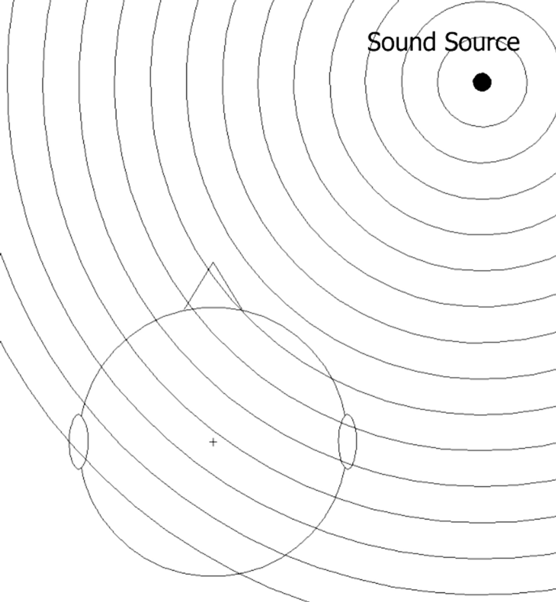
Figure 1. Sound waves arrive later at one ear compared to the other, depending on the location of the sound source. Since intensity is a function of distance from the sound source, it is obvious that the intensity level will also be different (from Miller and Matin [6]).
• Filter the signal as appropriate in order to account for head shadow, pinna effects, and cochlear implant processor;
• Compute FFT of the resultant signal in order to extract the phase and magnitude components;
• Identify dominant components regarding localization cues;
• Compute phase difference to extract the ITD;
• Using a vector model, determine the azimuth.
3.1. Head Shadow Effect
This component is responsible for generating the ITDs and ILDs caused by the shadowing effects of the head, which primarily impact high frequencies due to their small wavelength relative to the size of the head. ITD for a particular frequency is determined using Equation (1) below:
 (1)
(1)
where c is the speed of sound, TD is the time difference of the signal’s arrival, and f is the frequency of interest. This part of the model is very similar for both normal ears and cochlear implant users.
The first element is a simple pole-zero filter which is meant to approximate the Rayleigh spherical head model. It is parameterized by the angle difference between the
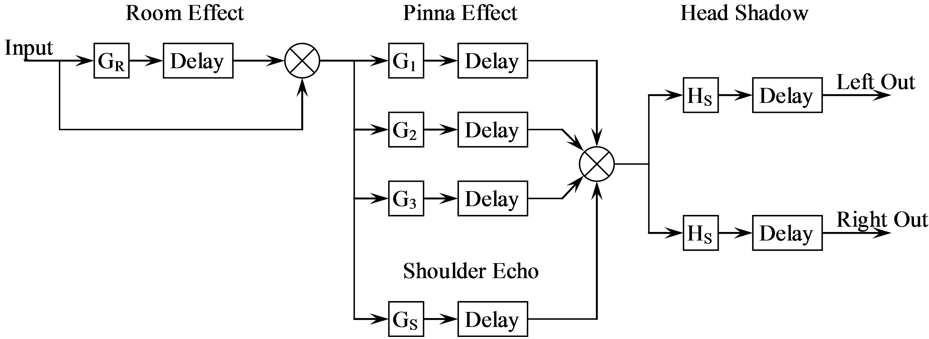
Figure 2. Block diagram of the head related transfer function algorithm (based on Brown and Duda [7]).
location of the ear and the azimuth of the sound source.
The gain of the low frequencies (below about 1500 Hz) is not drastically affected by head shadowing due to their longer wavelengths. To achieve this effect, the head shadow model has a fixed pole and a zero that moves to produce the desired amount of roll-off, depending on the azimuth of the sound source.
As part of the head shadow component there is a linear delay element. This accounts for the ITD produced by the waves propagating around a rigid sphere to reach the ear.
The pole zero filter suggested by Brown et al. [7] in their model is given by:
 (2)
(2)
where: m = speed of sound/radius of the head and
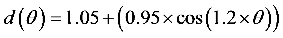 (3)
(3)
where θ is the angular difference between the location of the ear and the azimuth of the sound source.
The linear delay element for each ear (in seconds) is given by:
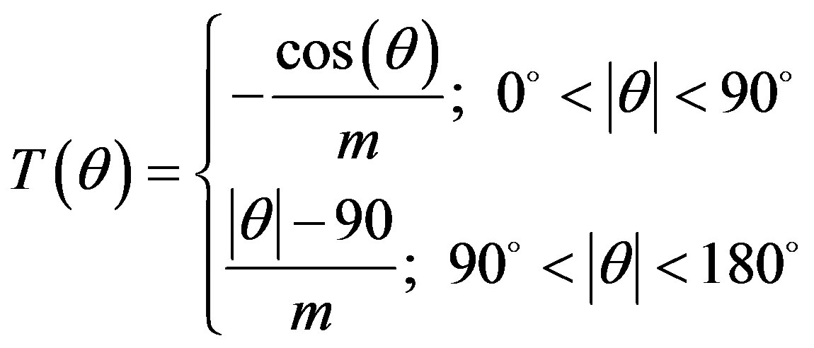
Figure 3 is graphical depiction of how vector elements are generated by the model in this implementation. It accounts for all aspects of the HRTF which will significantly affect the accuracy of the localization prediction.
3.2. Pinna Effects
Brown et al. approach [7] to developing a pinna (outer ear) model was to work only in the time domain. Their primary reason for working in the time domain is that
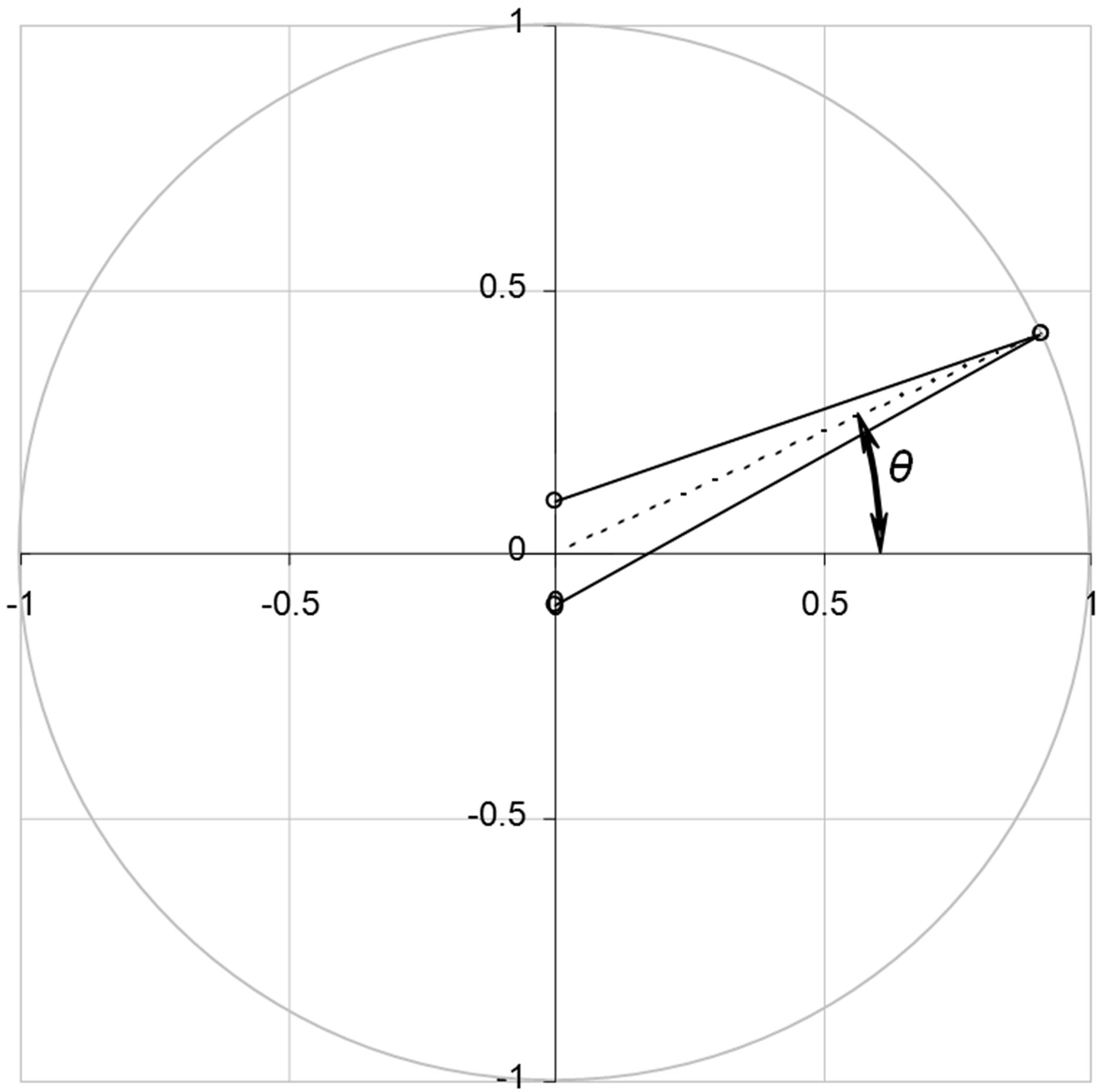
Figure 3. The solid lines represent the vectors corresponding to the signal paths from the target to the two ears. The dashed line is at the angle computed from the phase difference of the signal acquired at each ear (from Miller and Matin [6]).
many of the characteristics of HRTF’s are a consequence of sound waves reaching the ears by multiple paths. Sound that arrives over paths of different lengths interact in a manner that is obscure in the frequency domain, but is easily understood in the time domain. This greatly simplifies the structure of the model and reduces the computational requirements in implementing it.
To this end, the pinna effects were implemented in this model by constructing a 32-tap impulse response filter that incorporated the multiple echoes produced by an ideal pinna model. This was implemented in code in MatLab and placed in the signal path prior to the ITD determination and azimuth calculations.
3.3. Cochlear Implant Processing
For the cochlear implant model, the pinna effects block was replaced by transfer function similar to that commonly used in cochlear implant processors. In this case the signal is bandwidth-limited in the same manner that the CI processes the signal prior to encoding it as neural impulses to the auditory nerve in the cochlea. In a common CI processor, the signal is segregated by a filter bank into a number of frequency bins spanning the speech band of 200 Hz to 8 kHz. Of the 22 bins implemented, as for a common CI, the four bins containing the greatest amount of energy are then selected and that portion of the signal is passed on to be delivered to the auditory nerve.
The model mimics this process by implementing the same bank of bandpass filtering and bin selection, thus only allowing the localization algorithm to operate with this restricted band of acoustic information.
4. RESULTS
Cochlear implant processing, due to the nature of the neurological signal delivery system, strips all but the most important components of the signal and delivers only the most prominent elements. Figure 4 shows a spectral representation of a typical signal for normal hearing ipsilateral and contralateral ears. Figure 5 shows the spectral representation of that same signal that is delivered through a cochlear implant processor. One can clearly see that a great deal of spectral information is lost to the cochlear implant user.
The signal used when executing the model consisted of Maximum Length Sequences1 of 16,384 bit length played through a loudspeaker and recorded through KEMAR2 manikin ears. The spectral content of the signal generated in this manner is uncorrelated and broadband, thus fully exercising the full bandwidth of the model.
These plots demonstrate the spectral representation of the signal as detected by each ear as the azimuth is rotated from 0˚ to 180˚.
An analysis of the extracted phase angles was per-
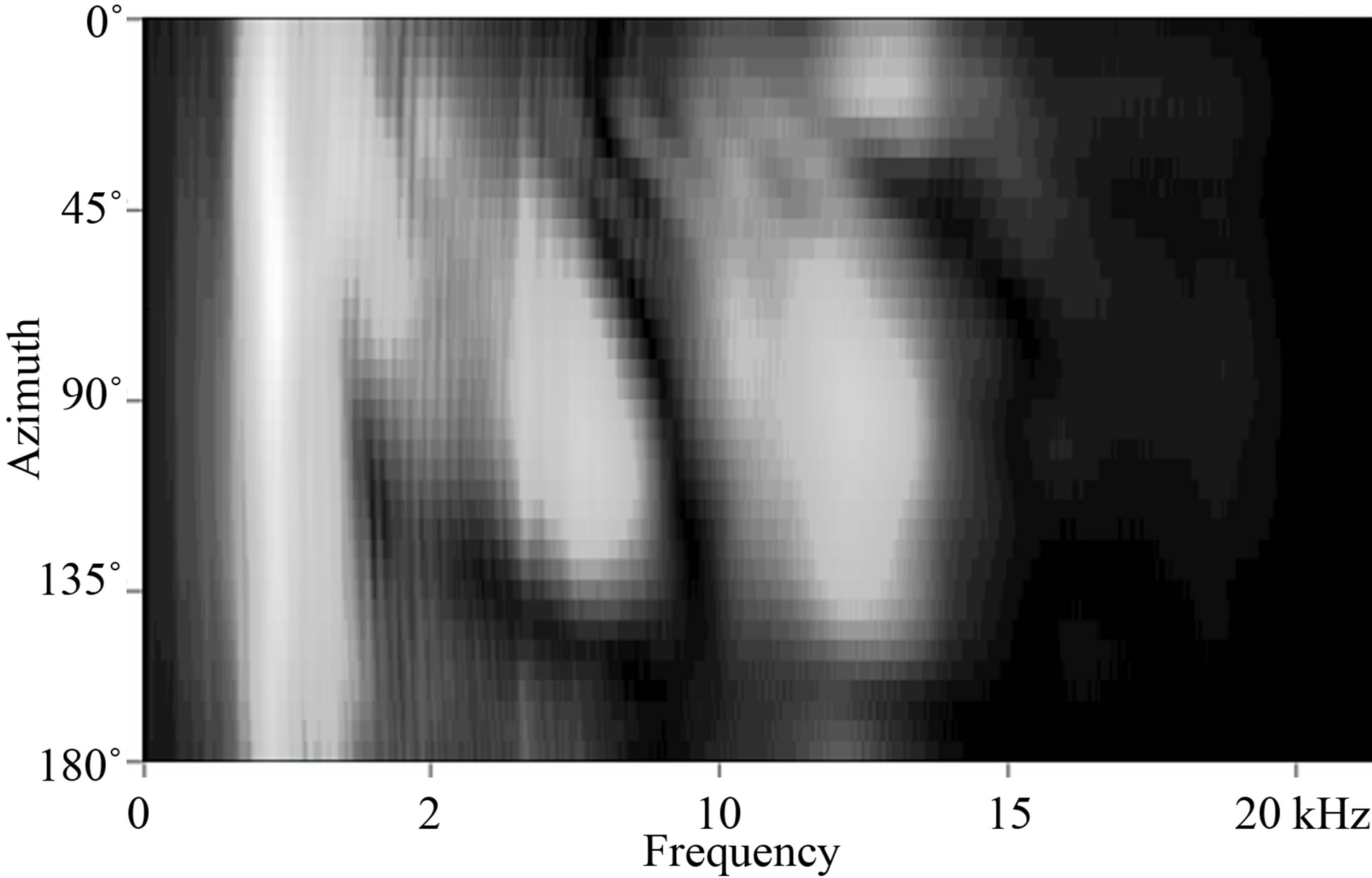
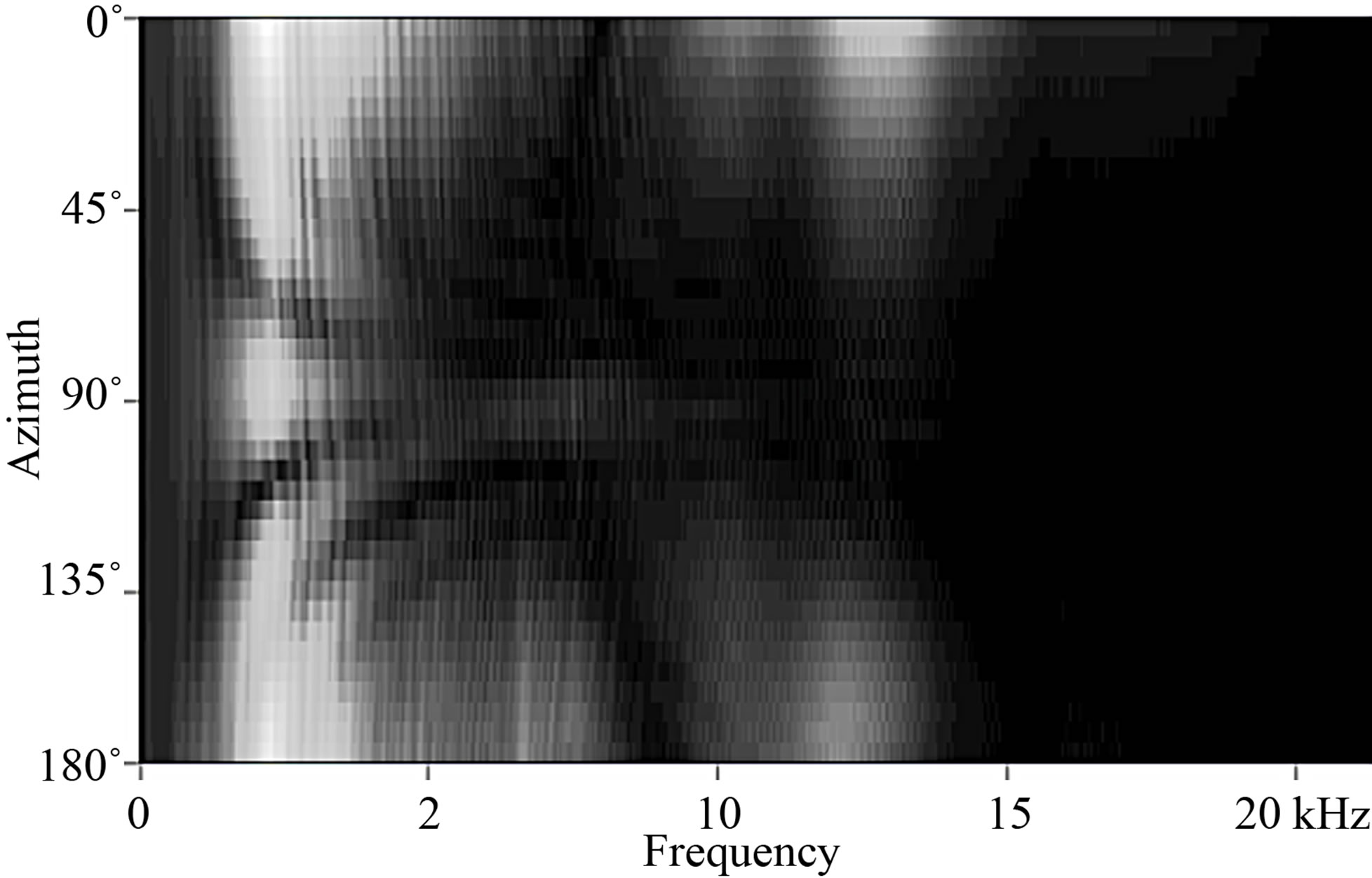
Figure 4. These plots demonstrate the spectral representation of the signal as detected by each ear as the azimuth is rotated from 0˚ to 180˚.

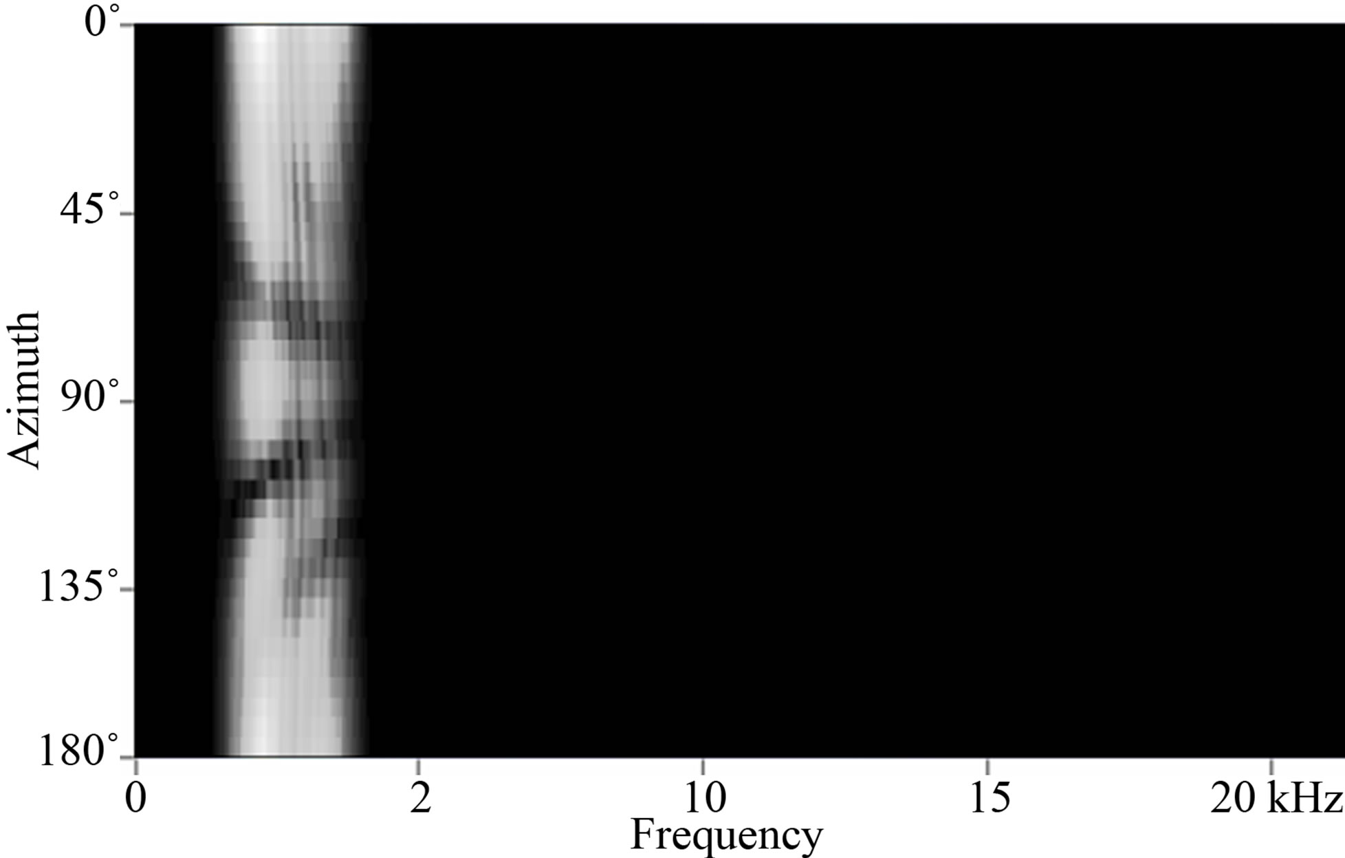
Figure 5. The spectral representation as experienced by a cochlear implant user for the same signal as presented in Figure 4. Clearly, the amount of information from which to make a localization determination is greatly reduced.
formed by the model on the resultant signals, shown in Figure 6, in order to determine the ITD. Further analysis was performed on the magnitudes of the signal so that differentiation could be made for azimuths with similar ITDs. With this ITD and ILD information, a determination of the direction to the source could be made.
The error was then calculated for each azimuth, and due to the granularity of the 5˚ azimuth steps, a smoothing function was applied to better represent the continuous error curve over the 0˚ to 180˚ azimuth range. This is shown in Figure 7 as the red curve for normal hearing and as the yellow curve for cochlear implant users.
In a study by Verschuur et al. [8], the authors reported that normal hearing subjects exhibited localization error of approximately 2˚ to 3˚. While van Hoesel and Tyler [9] reported cochlear implant subjects typically have poorer performance with an RMS Error of around 10˚ to 30˚. The performance of the normal hearing model presented in this paper exhibited an RMS Error of 3˚, and the cochlear implant model performed with an RMS Error of 23˚, both within the ranges reported in the literature for measured performance from normal hearing and cochlear implant human subjects. Table 1 shows a comparison of the model localization performance and that of the published data.
5. DISCUSSION
The RMS Error results achieved with the model developed in this work were similar for normal hearing subjects and for bilateral cochlear implant subjects published in the literature. The close correlation between published data on localization abilities of cochlear implant users and the modeled localization performance results in this study suggest that the poor performance is generally primarily due to the combination of differences in the HRTF of a normal hearing subject and a cochlear implant subject, and degradation of the cues by the signal processing of the implant.
An observation made concerning the localization error plot from the model was that localization by cochlear implant users appears to be poorer for anterior signal as compared to posterior signals. It is not clear from the published data to which this model was compared whether this was the case with tested subjects or not. It would be of interest to explore this further to determine whether this is actually the case, or if this is a quirk of the model.
A basic cochlear implant algorithm was used in this model, but is similar to one of the most commonly used. However, further work should be conducted using other commonly used signal processing strategies for which

Figure 6. Phase angles for the dominant spectral component at the ipsilateral (red) and contralateral (blue) ears. The green curve represents the phase differential as compared to the ideal represented by the gray line.
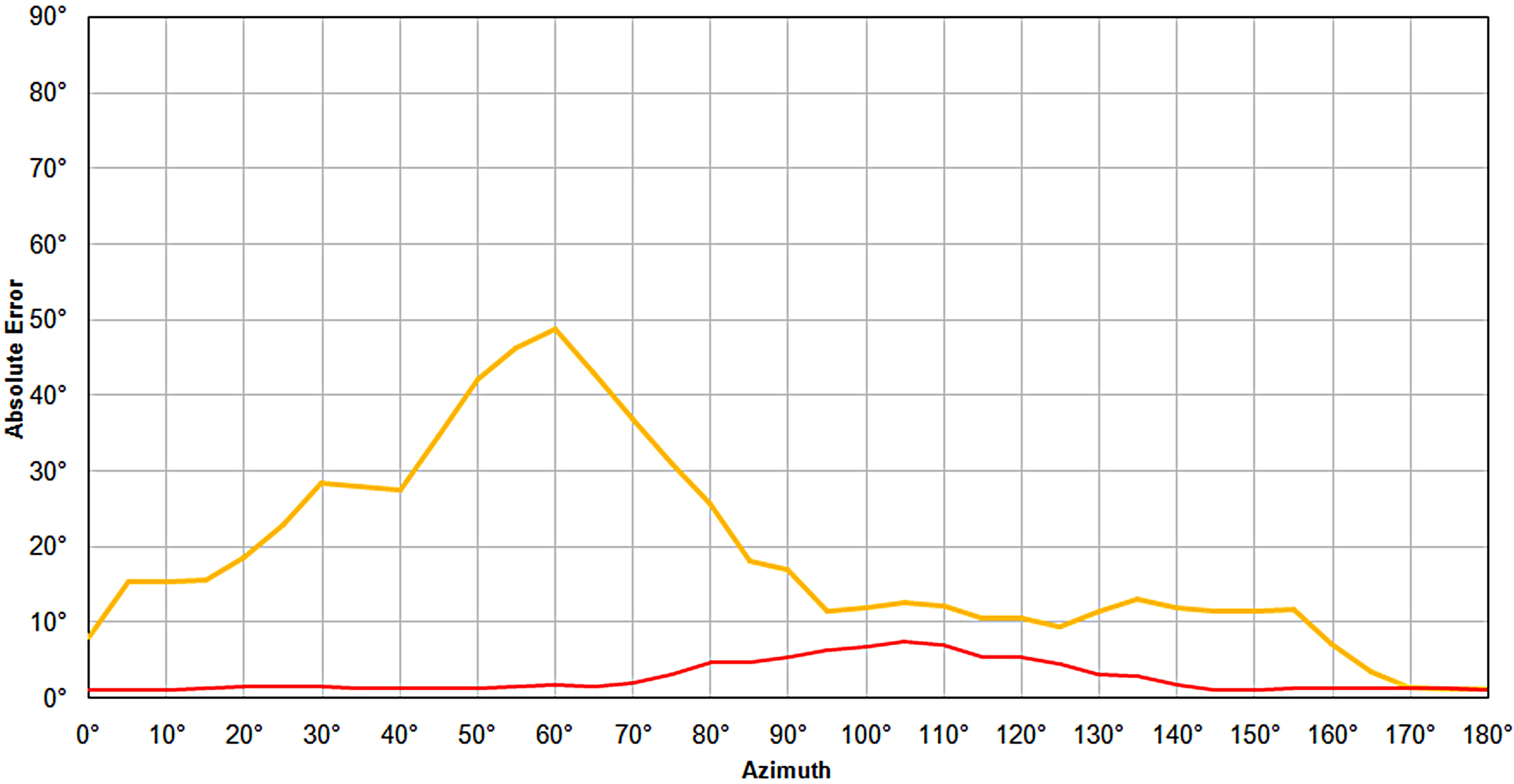
Figure 7. Localization error results obtained from the MatLab model. Since the modeled performance was generated in 5˚ steps in azimuth, a smoothing algorithm was applied in order to better represent the error responses in normal hearing and cochlear implant users. Cochlear implant error curve is yellow and normal is red.

Table 1. RMS Error of model compared to published data.
there is published localization data to determine if it predicts performance as well for them. In addition, there is room for improvement in the ILD analysis component of this model.
The ultimate goal of this study was to produce a model that could be used to assess the performance of newly developed signal processing algorithms in cochlear implant research. Thus the conducted work far suggests that this model could be used to predict a cochlear implant processing algorithm’s localization performance.
REFERENCES
- Durlach, N.I. and Colburn, H.S. (1978) Binaural phenomena. In: Carterette, E.C. and Friedman, M.P., Eds., Handbook of Perception, Vol. 4, Academic, New York.
- Bronkhurst, A.W. and Plomp, R. (1988) The effect of head-induced interaural time and level differences on speech intelligibility in noise. Journal of the Acoustical Society of America, 86, 1374-1383.
- Zurek, P. (1993) Binaural advantages and direction effects in speech intelligibility. In: Studebaker, G.A. and Hochberg, I., Eds., Acoustical Factors Affecting Hearing Aid Performance, 2nd Edition, Allyn & Bacon, Boston, 255-276.
- Shaw, E.A. (1974) Transformation of sound pressure level from the free field to the eardrum in the horizontal plane. Journal of the Acoustical Society of America, 56, 1848-1861. doi:10.1121/1.1903522
- Yost, W. and Dye. R. (1997) Fundamentals of directional hearing. Semin Hear, 18, 321-344. doi:10.1055/s-0028-1083035
- Miller, D.A. and Matin, M.A. (2011) Modeling the head related transfer function for sound localization in normal hearing persons and bilateral cochlear implant recipients. Proceedings of 14th International Conference on Computer and Information Technology (ICCIT 2011), San Diego, 22-24 December 2011, 344-349.
- Brown, C.P. and Duda, R.O. (1998) A structural model for binaural sound synthesis. IEEE Transactions on Speech and Audio Processing, 6, 476-488. doi:10.1109/89.709673
- Verschuur, C.A., Lutman, M.E., Ramsden, R., Greehan, P. and O’Driscoll, M. (2005) Auditory localization abilities in bilateral cochlear implant recipients. Otology & Neurotology, 26, 965-971. doi:10.1097/01.mao.0000185073.81070.07
NOTES
1Maximum Length Sequences are pseudorandom binary sequences are commonly used today for measuring acoustic characteristics due to their spectrally flat nature and because they provide recordings that are highly immune to external noise.