ABSTRACT

In one-dimensional multiparticle Quantum Cellular Automaton (QCA), the approximation of the bosonic system by fermion (boson-fermion correspondence) can be derived in a rather simple and intriguing way, where the principle to impose zero-derivative boundary conditions of one-particle QCA is also analogously used in particle-exchange boundary conditions. As a clear cut demonstration of this approximation, we calculate the ground state of few-particle systems in a box using imaginary time evolution simulation in 2nd quantization form as well as in 1st quantization form. Moreover in this 2nd quantized form of QCA calculation, we use Time Evolving Block Decimation (TEBD) algorithm. We present this demonstration to emphasize that the TEBD is most naturally regarded as an approximation method to the 2nd quantized form of QCA.

Keywords:

Quantum Cellular Automaton, QCA, Quantum Walk, Boson-Fermion Correspondence, Time Evolving Block Decimation, TEBD, Dirac Cellular Automaton

1. Introduction

Quantum Cellular Automaton (QCA) [1] is a quantum version of (classical) cellular automaton (CA). The word QCA was introduced by Grössing and Zeilinger [2] . But their model was not completely unitary. The QCA in the right meaning which has both locality and unitarity, was firstly investigated by Meyer [3] [4] [5] [6] , then followed by Boghosian and Taylor [7] [8] , though they used the term Quantum lattice gas automata (QLGA) for the two-component case. Since the middle of the 2000 s, new axiomatic approaches of QCA different from previous conventional or ad hoc ones have been proposed by several researchers [9] [10] [11] in order to comprehend QCA in more systematic and unified way by clarifying the definitions and/or to cope with the difficulties for extending it in a form relevant to the infinite dimensional Hilbert space. In most axiomatic QCAs, the unitarity and the causality (namely the existence of the upper limit on the speed of the information propagation) are fundamental and the locality is derived from them [10] . In this study, however, we describe QCA in a rather conventional fashion. There are several frameworks for quantum lattice systems other than QCA, namely Quantum Walk (QW) [12] , Quantum Lattice Gas Automata (QLGA) [7] [8] and Quantum Lattice Boltzmann (QLB) [13] . They are similar or mathematically equivalent to some QCAs [14] [15] . As QW and QLGA are thought to be subclasses of QCA [16] , we use the term QCA if at all possible.

QCA can be regarded as a discrete mechanical system with a simple and elegant time evolution rule. Though it is simple, it is not just a toy method. It can simulate the real quantum system of matter. Moreover there are several ideas that QCA plays a key role in fundamental physics [17] [18] and extensions to nonlinear QCA have been studied [19] which might be clues to constructing some class of interacting multiparticle QCA models.

QCA can be also regarded as one of the approximation methods for solving the continuous Time Dependent Schrödinger Equation (TDSE) like Finite Difference Method (FDM). However QCA is unique in that it preserves the complete unitarity of quantum systems upon its time progression and it can be regarded as the discrete version of direct solution for quantum dynamics, not merely an approximation to the TDSE. TDSE emerges rather as an approximation in the zero wavenumber limit of the general QCA solution. By extending the one-particle QCA to many-particle QCA, we explore the possibility of the method in real quantum systems.

The Time Evolving Block Decimation (TEBD) [20] [21] is one of the most successful methods to simulate quantum many-body systems. We however emphasize that it can be regarded as an approximation to the 2nd quantized form of QCA. In this study, we discuss the TEBD from the QCA point of view.

Since the success of Density Matrix Renormalization Group (DMRG) [22] , Matrix Product State (MPS) has been recognized as an efficient mathematical means for describing (quasi) one dimensional quantum many-body systems. The MPS is used both in eigenstate search by imaginary time evolution and in real time evolution of general states. TEBD is one of the standard algorithms in imaginary or real time evolution of MPS. The first part of TEBD algorism is to divide the Hamiltonian into even part and odd part, then the split-step or Suzuki-Trotter formalism is applied, namely the exponential of the even part or that of the odd part is applied alternatively to the 2nd quantized wavefunction. When we use the usual hopping term in the Hamiltonian as the kinetic energy part, this first part of TEBD can be regarded as 2nd quantized form of QCA. This QCA form seems to be a byproduct of the 2nd order Suzuki-Trotter decomposition or just an approximation method to the TDSE. In this study we however emphasize that it is more natural or fundamental to regard the one-particle QCA as the starting point of TEBD algorism in order to directly obtain the solution for general quantum systems.

The boson-fermion correspondence in the one dimensional quantum system is well known. However in studying QCA-TEBD formalism we notice that this can be derived in a rather simple and intriguing way. The main purpose of this study is to show this simple derivation and application to few body systems of boson. Numerical studies on applicable range of the “boson approximation” (approximation of the bosonic system by fermion) are also performed.

2. First Quantized Form of QCA

2.1. One-Particle QCA

Consider the simplest partitioned QCA on a 1D-time 1D-space lattice of which time evolution rule is given by Figure 1 and Equation (1) (for TDSE-type QCA). This rule is governed by the 2 ´ 2 basic unitary matrix (which is called scattering unitary matrix [11] ) which operates on a vector consisting of functions at adjacent grid points.

(1)

Here is the x-component of Pauli matrices and.

is the parameter of the TDSE-type QCA.

Though it is not straightforward to recognize intuitively, QCA gives a solution of the free particle TDSE in the zero wave number limit.

(2)

The relation between mass and (the parameter of TDSE-type QCA) is given by

(3)

This relation can be obtained by several methods as we will mention later. We introduce a simple derivation using FDM for small as follows.

By replacing the spatial derivative with the spatial difference, Equation (2) becomes

(4)

Here is the 2nd order central difference operator defined by

(5)

where S is the one-grid shift operator

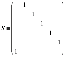(6)

(Here we use 6 ´ 6 matrices assuming that the system consists of 6-grid points with periodic boundary condition. Moreover unfilled matrix elements are assumed to be zero throughout this article.)

Therefore the time evolution for the time step is given by

(7)

This is approximated according to individual time-discretization schemes of FDM. For example the simplest but less accurate scheme is Forward Euler method, where it is approximated as. In QCA however is approximated in a different way. Firstly is divided into two parts.

(8)

where

Then is approximated as a split-step form

(9)

Note that as have a 2 ´ 2 block diagonal form, their exponential can be explicitly calculated. In this way the time evolution for is

divided into two steps ,so we naturally define as the time step of QCA and is expressed as using this definition, which corres-

ponds to Equation (3) for small.

The QCA dynamics obeys such a simple rule above. However it requires more elaborate techniques to derive the exact relation between mass and QCA parameter in general case Equation (3). This FDM-QCA correspondence is essentially the same as the first part of TEBD algorism we discuss later.

There are several approaches to obtain the continuous limit (namely PDE) of QCA. The most naive and straightforward one is to connect the discrete time to continuous time by the interpolation and then to take a wavenumber (k) expansion around k = 0 in the spatial direction [23] [24] [25] . Although this approach lacks some exactness, it is sufficient to obtain right TDSE characteristics. More precise approach is to use a single scaling parameter on which other parameters (etc) are defined to depend properly such that limit exists [8] . Another approach is to use a “path integral” on a lattice to obtain a discrete Green function then take an appropriate limit [3] . Using these approaches one dimensional Dirac equation (for mass) can be derived in the

limit. Another recent study can be found in [26] . In this study we do

not get into detailed derivation leading to the Dirac equation, as we are interested here in nonrelativistic case, though we will discuss a relevant topic in the last supplementary section.

2.2. Boundary Condition for QCA

There are basically three easily implementable boundary conditions for QCA. These are illustrated in Figure 2. In the cases of (2) (3), the evolution rule at a boundary point(x = 0 or x = N − 1) in odd time is only to multiply the phase rotation factor as shown below. (We show only the case x = 0 as the case x = N − 1 is essentially the same).

For zero derivative boundary condition [(2)], phase rotation factor is 1 as

(10)

For zero amplitude boundary condition [(3)], phase rotation factor is as

(11)

Note that the unitarity is always satisfied, because the probability increase and decrease are balanced between left and right boundary grid points in the case of (1) and they are zero in the case of (2) (3).

Boundary conditions and discontinuities (inhomogeneities) for QCA are firstly investigated by Meyer. He investigated more general 2-component QCA having two angle parameters. The scalar QCA we use is the simplest one having only one angle parameter, which corresponds to one of factors if his QCA is flattened (namely changed from 2-component to scalar by doubling the number of grid points) and is factorized [23] (2-step QCA of Section 6).

2.3. Multidimensional QCA

It is straightforward to construct multi-dimensional QCA. We have only to use direct product of 2 ´ 2 local unitary 1D matrices to generate 2D matrices.

(12)

The rule is illustrated in Figure 3. Concretely

(13)

(where x, y are even if t is even, and x, y are odd if t is odd.)

As we know each U approximately corresponds to the evolution

or and they commute with each

other, approximately corresponds to the evolution

, namely it causes 2D free TDSE time evolution. We thus

generate multidimensional QCA for general dimension.

Applications of QCA to multidimensional cases are studied in [7] [8] [9] . In multidimensional QW, less straightforward (namely not direct product) models are mainly studied, where the number of internal states is not (D: the dimension of the space) but less than this (for example 2, 4) [24] [25] .

2.4. Multiparticle QCA

It is also straightforward to construct (non-interacting) multiparticle QCA. D- dimensional distinguishable M-particle system is equivalent to DM-dimensional 1-particle system. For indistinguishable particle systems, we have to restrict this space to symmetric or anti-symmetric subspace according to the statistics of the particles. Note that preserve this symmetry for the case of distinguishable particle systems and we can define for the subspace of indistinguishable particle systems. (Here U means global unitary matrix, not 2 ´ 2 local unitary matrix)Applications of QCA to multiparticle cases are studied in [3] [7] [8] [9] .

3. Second Quantized Form of QCA

3.1. Concrete Evolution Rule of 2nd Quantized QCA

If the one-particle time evolution rule is given by an infinitesimal time evolution matrix, namely, a generator or a Hamiltonian, it is straightforward to construct a 2nd quantized Hamiltonian for its free particles.

(14)

(Here is the 1-particle Hamiltonian matrix elements, are the creation and annihilation operators for Boson).

If the one-particle time evolution rule is given not by a generator but by a finite time evolution matrix such as in QCA, the construction of its 2nd quantized formalism is done in a slightly different way, which though is consistent with the generator case. For example the evolution of 3-particle state is described as follows

(15)

Namely we can apply the substitution rule

(16)

We now apply this substitution rule to 1D free bosonic QCA system where unitary transformation only between nearest neighbor grids occurs, and the one step evolution is given by

(17)

The explicit local unitary evolution matrix for the grid pair is

18)

(local unitary matrices for other grid pairs have the same form).

We then apply the substitution rule to 1D free fermionic QCA system. Focusing on the grid pair, four states evolve as follows.

(19)

Here and are fermion creation operators fulfilling anti-commutation. Namely, the local unitary evolution matrix is

(20)

It should be noted that if periodic boundary condition is adopted for the grid pair, the off-diagonal element in Equation (20) must be replaced with considering that etc. (M is the total number of particles in all grid points.) Essentially same equation as Equation (20) is proposed in other literatures on multiparticle QCA [3] [8] [9] .

3.2. MPS Approximation of QCA

Now we introduce an interaction between particles. For this purpose, it is reasonable to introduce an additional phase rotation factor by the potential caused by other particles just like the external potential case.

Note that QCA with external potential was firstly studied by Meyer [4] . QCA with the nearest neighbor pair interaction was studied also by Meyer [3] and Boghosian [8] and Schumacher and Werner [9] in the form we present here.

Here we discuss the simplest case, namely the cases where the nearest neighbor interaction is included. We assume that interaction occurs as an additional phase rotation only when two particles exist in the neighboring grids. In the context of QLGA (two-component QCA), this additional phase rotation corresponds to the phase shift by the collision between the left-going and the right going particles [3] . Under this assumption, the 4 ´ 4 local unitary evolution matrix becomes

(21)

Here meansattraction, and means repulsion.

Note that in this simplest case, the structure of evolution scheme is kept same as the structure of free fermion case. After preparing this form, we can apply a MPS approximation and a usual TEBD algorism illustrated by Figure 4 and Figure 5. A general wave function for the 2nd quantized form of QCA is approximated by MPS as

(22)

(for the 8 grid points case, m is the dimension of auxiliary spaces and the shape of tensor is (2,m) for i = 0, (m,2,m) for i = 1 to 6, (m,2) for i = 7), then upon the time evolution, each adjacent pair of are updated by applying the 4 ´ 4 unitary matrix U of Equation (21) as

(23)

Here SVD is applied then the subspace corresponding to small singular values is truncated in order to keep the dimension of auxiliary space to the given value (m in this case).

For zero derivative or zero amplitude boundary condition, at an odd time, the end points are updated by applying the 2 ´ 2 diagonal unitary matrix. for zero derivative or zero amplitude boundarycondition respectively.)

Finally in this section, we compare our method with the ordinal way of reaching the TEBD algorithm. Basically so called hopping term representing kinetic energy part in evenly-spaced-grid-base (or site-base) quantum models such as Hubbard model or fermionized XXZ model is derived from the FDM-ap- proximation of kinetic energy term. The FDM-approximated Hamiltonian matrix of one-particle TDSE is given by

(24)

(Here is the external potential at the position x.)

And, its 2nd quantized Hamiltonian for non-interacting fermions is

(25)

(The 1st term is so called hopping term. is the total particle number and here we assume it constant).

By adding neighboring interaction term and dropping external potential term and constant term for simplicity, we have fermionized XXZ model [27] [28] , where only nearest neighbor grid point of occupation number have a interaction through.

(26)

If the anisotropy parameter, this model corresponds to the XXX model for fermion where the interaction is two-body coulomb interaction.

The XXZ spin model and its equivalent fermionized version are well studied [27] . The phase diagram of the XXZ spin model in extended systems with the external magnetic field consists of 3 phases, ferromagnetic, paramagnetic and antiferromagnetic phases. When the magnetic field is zero, correspond to ferromagnetic (gapped), paramagnetic (gapless) and antiferromagnetic phases respectively and in the paramagnetic phase, quasi particles (magnon) behave as boson-like Tomonga-Luttinger liquid [29] [30] . The magnetic field in the XXZ spin model becomes the chemical potential when the model is fermionized. The method has been used for grand canonical systems. We however focus our application in finite system where the number of particles fixed.

According to the TEBD algorism, we decompose the Hamiltonian into two parts.

(27)

Time evolution during the small time interval is done as follows (Suzuki-Trotter)

(28)

As terms in or commute with each other, we have

and

(This is QCA-like evolution). As each factor is finite matrix, we can obtain easily its matrix representation using the standard matrix representation of creation and annihilation operator as follows.

(29)

(30)

We see the exact correspondence of the hopping term parameter in the model Hamiltonian to the QCA parameter, and the strength of correlation introduced by can be interpreted as the phase factor caused by the local potential at the grid point from the other electron in QCA. When, namely, it corresponds to the free Boson approximation case we will address in the next section.

4. Boson Approximation by Fermionic QCA

4.1. Formalism

As shown in Equation (18) and Equation (20), the grid pair evolution matrix for bosonic QCA is infinite size matrix, whereas that of fermionic QCA is reduced to 4 ´ 4. It is desirable if bosonic QCA is well approximated by a QCA with small degree of freedom as in the fermionic QCA.

We propose here boson approximation by fermionic QCA (or QCA with a hard core condition) when occupation number per grid is small. We mean by the hard core condition that at most one-particle can reside in one grid point. (We not necessarily mean). We assume that only the amplitudes at points where all are different comprise the full set of independent variables and amplitudes of other points (etc.) needed for evolution are evaluated by interpolation from other points (set to the value of nearby point.) We illustrate in Figure 6 the method of the boson approximation we propose for two-particle case, comparing with free fermionic QCA case.

In order to make it easy to understand, we compare with the free fermion case, where no interpolation is needed, namely we set the amplitudes where to zero. For example, in 2-particle free fermion case, must be anti-

symmetric with respect to exchange of. And we can obtain the evolution rule at a quadrilateral on the diagonal line as follows.

(31)

(where we set)

For 2-particle Boson approximation case, must be symmetric with respect to exchange of, but the amplitude cannot be given without some assumptions. We take an approximation to assume that

(32)

Under this assumption, we have the following evolution rule.

(33)

This implies, the 4 by 4 Unitary matrix in 2nd quantization formalism changed from that of Fermion case as follows

(34)

As mentioned before, this 4 ´ 4 unitary matrix is the same as that of the fermion system (fermionized XXZ) with nearest neighbor attractive interaction (namely fermionized XXX). This means that fermion-boson correspondence for this 1D quantum system is easily derived from the QCA-TEBD formulation.

We give another possible interpretation of Equation (34). The boson approximation Equation (34) can be obtained by applying coarse graining to Equation (18) using the following seemingly reasonable weight matrix for the adjacent grid pair subspace. Namely the 11 - 11 component of Equation (34) (=1) is obtained also by

(35)

Here, coarse graining means that three states of the adjacent grid pair, namely, are joined into one state (1,1) so that the occupation number per grid is kept less than 2 upon time evolution. Note that the original bosonic QCA Equation (18) does not conserve hard core condition due to the transition from to (0,2) or (2,0).

4.2. Sample Simulation

Here we show examples of the QCA-TEBD application with the boson approximation. In our simulations, we adopt the minimal auxiliary space dimension for MPS which can describe any 1-slater wavefunction (namely for M particle system). 2nd-quantized MPS-form wave function describing 1st-quantized 1- slater wave function for M particle N grid point system can be given as follows using representation matrices of creation and annihilation operators and orthonormal orbitals (i = 0 to: occupied orbital number).

(36)

(37)

We can verify that

(38)

For example, in 2-particle case, using the standard representation of Fermion creation and annihilation operators

we have

(39)

We simulated 2-particles in a one-dimensional box using imaginary time evolution.

At t = 0 we set 2-particles at adjacent two grid points near the center position.

In Figure 7 we show converged density distributions for N = 64,256 and cases. For (free fermion), it converges to the state where the two particles occupy the ground and the 1st-exited (1-particle) states.

(40)

For (free boson approximation), it converges to the state where the two-particle reside in the same (1-particle) ground state.

(41)

Similarly we computed MPS wave function for the three particle system and the results are shown in Figure 8.

In general the parameter of the interaction must be scaled properly when the grid spacing is changed in order to obtain the same continuum limit waveform. It is reasonable that when the ground state waveform does not depend on N, and when it depends on N. The case of is exceptional in that the waveform does not depend on N as if the particles were not interacting despite the fact that interaction is taken into account by non-zero parameter. This reflects the validity of the boson approximation.

In Figure 9 we show the ratio of sum of the truncated norms of singular values to that of all singular values for N = 64,256 and cases. Ratios

are sufficiently small and MPS approximation must be good for the case. Theoretically the ratio should be zero for the free fermion case, but small numerical error is observed.

In Figure 10, we show the converged density distribution of two-particle system.For the case, the discontinuity of the wave funcion can be seen at. In general the boson approximation wavefuncion and the real fermionic wavefunction are thought to be related by Equation (42) [31] .

(42)

where

Finally we provide here more detailed information about simulation methods

we adopted, though this is not the main purpose of this study. To perform imaginary time simulation, we set simply in the unitary matrix Equation (30) to the imaginary value. We performed a canonicalization of MPS state proposed by Vidal [21] at each simulation step, and in addition to this we performed an appropriate gauge transformation of MPS state corresponding to an additional evolution by the spatially constant chemical potential. In a MPS simulation of systems of fixed particle numbers, the chemical potential is theoretically irrelevant to the result, but it affects the robustness of the simulation and a small numerical error causes violation of particle number conservation leading to the grand canonical ground state.

5. Simulation by 1st Quantized Form of QCA

In this section we explain how to perform the equivalent simulation by the 1st

quantized form of QCA. Of course in contrast to the above QCA-TEBD simulation, this can be performed only when the number of grids or particles is small (notorious exponential wall for large number problems) . But as it is simple and free from the particle number conservation problem, the result can be used as a reference to the QCA-TEBD simulation. Moreover there are no fundamental difficulties, in simulating bosonic or higher dimensional systems by the 1st quantized form. We already explained the relation between the 1st quantized QCA and the 2nd quantized QCA in the free particles case, we here explain how to treat the additional phase rotation caused by interactions in the 1st quantized QCA. Firstly we explain the 1D-2 particle case. One step evolution is given by Equation (43).

(43)

At an even or odd time the evolution rule Equation (43) is applied to each even or odd quadrilateral (namely red or blue quadrilateral in Figure 6) respectively. Precisely the rule Equation (43) is for the bulk. At the zero boundaries the application of U in are (partially) replaced by the simple phase rotation of Equation (11) at an odd time.

The algorithm of the 1st quantized form of QCA is basically independent of particle statistics. The only procedural difference between boson and fermion is in symmetrization or anti-symmetrization at each simulation step. Without this anti-symmetrization however a decay from a fermionic state to a bosonic state occurs occasionally.

In more general 1D M-particle case, in Equation (43) becomes. For example, at the point in 1D 4-particle case, the additional phase rotation at an even time is which comes from and .

In higher dimensional case, the free evolution part is the same as in 1D case, and only the paring condition for the additional phase rotation need to be modified except for the obvious (anti)-symmetrization procedure.

In a case of higher dimension or many particles, the requirement for the magnitude of becomes severe. If we set upper bound of phase rotation per

one simulation step to, then is required for the zero boundary condition and is required. (Here D is the dimension of the

space and is the maximum number of nearest neighbor pairs, especially

for 1D fermion case.)For the more practical programing, we reserve

the memory only for the simplex region taking advantage of the (anti-) symmetry of the wave function though it requires a little bit care.

In the following, we show two imaginary time 1st quantized QCA simulations, one is 1D 4 particle fermionic and corresponding bosonic system, the other is 2D 2 particle fermionic and bosonic systems.

The Hamiltonians related to the fermionic and bosonic QCAs we simulate are

(44)

(45)

where means nearest neighbor pairs (Note that in 1D fermion case Equation (44) is the rewritten Hamiltonian of the fermionized XXZ model using).

We show the result of 1D 4 particle and 2D 2particle imaginary time simulations in Figure 11 and Figure 12 respectively. We already showed in QCA-TEBD simulation that the fermionic 1D system with behaves approximately the same as the 1D free bosonic system. More generally, by adding extra phase rotation caused by neighboring grid pair interaction, we conclude that

the 1D fermionic system with behaves approximately the same as the 1D bosonic system with. In Figure 11 we confirm that this approximation is very good for. (Note that similar boson-fer-mion correspondence for 1D continuous space quantum system is well known, namely, the bosonic system with infinite repulsive delta function behaves as a free fermion [31] [32] ).

By seeing Figure 12 one might expect that fermionic 2D system with behaves approximately the same as the 2D free bosonic system, but in more than 1D system, there is no such a simple correspondence between fermion and boson as 1D system, because collision points are qualitatively different from boundary points in more than 1D system.

In Figure 13 we show the applicable parameter range of boson approximation in 2/3/4 particle systems. For 1-body-reduced density distribution for bosonic system are well approximated by that of fermionic system when. But after exceeds 1 the error becomes rapidly larger. For 2-body-(reduced) density distribution, the error increases rapidly when reaches slightly below 1. In the condensation state, the assumption used for the wave function interpolation seems to become inapplicable.

6. Multi-Step QCA and Dirac Cellular Automaton

In this supplementary section, we briefly discuss the possibility of multi-step QCA. Firstly we discuss QW and Dirac Cellular Automaton (DCA) [25] [33] [34] as special cases of multi-step QCA. The 1D simplest (namely having only one 2 × 2 unitary matrix as parameters) QW/DCA are mathematically equivalent

to the corresponding QCA. This equivalence is easily shown by using the factorization form of the two-grid translationally invariant banded unitary matrix (namely multi-step QCA form) [9] [23] . In order to interpret QW/DCA as QCA, they are flattened to scalar models as shown in Figure 14.

Namely their two components (up and down) are assigned to two amplitudes of adjacent grid points in the lattice of which the number of grid points are doubled from the original lattice. The 2 ´ 2-unit Z-transformation representation [23] of QCA, QW and DCA are given as

(46)

(47)

(48)

respectively. Here are general 2 ´ 2 Unitary matrices,

is the parameter of the 2 ´ 2-unit Z-transformation which means two-grid

shift in the flattened lattice and is the 2 ´ 2-unit Z-transfor-

mation representation of the one-grid shift matrix defined by Equation (6). Note that, therefore commute with any 2 ´ 2 matrix.

Now we rewrite in a factorization form.

(49)

Considering we have

(50)

(51)

where. (The expressions in the parentheses of Equations (50)

(51) are added in order to clarify the correspondence between the expressions and the graphs in Figure 14.

By taking the logarithm of (see for example [23] ) we can obtain TDSE or 1DDirac equation from TDSE-type QCA as its continuum limit. However in this case, obtained 1DDirac equation is not ideal one. In the QW case, the situation is the same. In the DCA case, the more ideal 1DDirac equation emerges. In the following we explain the outline of this situation. In the QCA case, we parametrize the basic 2 ´ 2 unitary matrix as follows.

(52)

The corresponding Hamiltonian is

(53)

(54)

where

(55)

The case (where has the form) is particularly simple and important and we restrict our argument to this case.

are the typical cases of

.

In order to be able to connect this QCA with the Dirac equation, in the wave number expansion

(56)

must be traceless (namely their squares are scalar multiples of I) and which are indeed satisfied. Moreover it would be ideal if. Although actually in all cases by similar calculations, only in

the DCA case when k-dependence of is ignored, which makes

DCA more suitable in connecting to Dirac equation.

As we explained above (Equations (50) (51) and Figure 14), the TDSE/Di- rac-type QW/DCA can be regarded as special case of two-step QCA and moreover mathematically equivalent to two sets of TDSE-type single-step QCAs. Therefore the same arguments about the boundary condition, the 2nd quantiza- tion formalism, the simplest interaction and the boson-fermion corresponding as in QCA apparently hold. Moreover in TDSE/Dirac type multi-step QCA the similar argument would be possible, though we need more investigation about what essentially new phenomenon could appear by extending the single-step QCA to the general multi-step QCA (Equation (49)).

7. Conclusion

In this study we show that in one-dimensional multiparticle QCA, the approximation of the bosonic system by fermion (boson-fermion correspondence) can be derived in rather a simple and intriguing way, where the principle to impose zero-derivative boundary conditions of one-particle QCA is also analogously used in particle-exchange boundary conditions. As a clear cut demonstration of this boson approximation, we calculate the ground state of 2 or 3-particle systems in a box using imaginary time QCA-TEBD simulation. Obtained ground states are indeed boson-like. We also perform imaginary time simulations by the 1st quantized form of QCA not only for fermionic system but also for bosonic system and show the applicable range of boson approximation (boson-fermion correspondence). Another point we want to emphasize throughout this study is that QCA, TEBD (MPS), FDM are deeply related to each other. The 1st quantized form of QCA can be regarded as the split step decomposition of FDM description for TDSE, which is essentially the same approximation used when TEBD algorithm is obtained from the model quantum Hamiltonian system with nearest neighbor interaction. On the other hand, the 2nd quantized form of QCA has the TEBD form from the beginning.

Acknowledgements

This work was supported by Education Center for Next-generation Simulation Engineering, Toyohashi University of Technology and University-Community Partnership Promotion Center, Toyohashi University of Technology. We would like to thank Prof. Hitoshi Goto for his support and Dr. Akira Saitoh for his helpful advice.

Cite this paper

Hamada, S. and Sekino, H. (2017) The Approximation of Bosonic System by Fermion in Quantum Cellular Automaton. Journal of Quantum Information Science, 7, 6-34. https://doi.org/10.4236/jqis.2017.71002

References

- 1. Wiesner, K. (2009) Quantum Cellular Automata. In: Meyers, R.A., Ed., Encyclopedia of Complexity and Systems Science, Springer, New York, 7154-7164.
https://doi.org/10.1007/978-0-387-30440-3_426 - 2. GrÖssing, G. and Zeilinger, A. (1988) Quantum Cellular Automata. Complex Systems, 2, 197-208.
- 3. Meyer, D.A. (1996) From Quantum Cellular Automata to Quantum Lattice Gases. Journal of Statistical Physics, 85, 551-574.
https://doi.org/10.1007/BF02199356 - 4. Meyer, D.A. (1997) Quantum Mechanics of Lattice Gas Automation: One-Particle Plane Waves and Potential. Physical Review E, 55, 5261-5269.
- 5. Meyer, D.A. (1998) Quantum Mechanics of Lattice Gas Automata: Boundary Conditions and Other in Homogeneities. Journal of Physics A, 31, 2321-2340.
https://doi.org/10.1088/0305-4470/31/10/009 - 6. Meyer, D.A. (1997) Quantum Lattice Gasses and Their Invariants. International Journal of Modern Physics C, 8, 717-735.
https://doi.org/10.1142/S0129183197000618 - 7. Boghosian, B.M. and Taylor IV, W. (1998) Quantum Lattice-Gas Model for the Many-Particle SchrÖdinger Equation in D Dimensions. Physica Review E, 57, 54-66.
https://doi.org/10.1103/PhysRevE.57.54 - 8. Boghosian, B.M. and Taylor IV, W. (1998) Simulating Quantum Mechanics on a Quantum Computer. Physica D, 120, 30-42.
https://doi.org/10.1016/S0167-2789(98)00042-6 - 9. Schumacher, B. and Werner, R. (2004) Reversible Quantum Cellular Automata.
- 10. Arrighi, P., Nesme, V. and Werner, R. (2011) Unitarity plus Causality Implies Localizability. Journal of Computer and Systems Science, 77, 372-378.
https://doi.org/10.1016/j.jcss.2010.05.004 - 11. Arrighi, P. and Grattage, J. (2012) Partitioned Quantum Cellular Qutomata Are Intrinsically Universal. Journal of Natural Computing, 11, 13-22.
https://doi.org/10.1007/s11047-011-9277-6 - 12. Venegas-Andraca, S.E. (2012) Quantum Walks: A Comprehensive Review. Quantum Information Processing, 11, 1015-1106.
https://doi.org/10.1007/s11128-012-0432-5 - 13. Succi, S. and Benzi, R. (1993) Lattice Boltzmann Equation for Quantum Mechanics. Physica D: Nonlinear Phenomena, 69, 327-332.
https://doi.org/10.1016/0167-2789(93)90096-J - 14. Succi, S., Fillion-Gourdeau, F. and Palpacelli, S. (2015) Quantum Lattice Boltzmann Is a Quantum Walk. EPJ Quantum Technology, 2, 12.
https://doi.org/10.1140/epjqt/s40507-015-0025-1 - 15. Hamada, M., Konno, M. and Segawa, E. (2005) Relation between Coined Quantum Walks and Quantum Cellular Automata. RIMS Kokyuroku, 1422, 1-11.
- 16. Shakeel, A. and Love, P.J. (2013) When Is a Quantum Cellular Automaton (QCA) a Quantum Lattice Gas Automaton (QLGA)? Journal of Mathematical Physics, 54, Article ID: 092203.
- 17. Hooft, G. (2014) The Cellular Automaton Interpretation of Quantum Mechanics. A View on the Quantum Nature of Our Universe, Compulsory or Impossible?
https://arxiv.org/abs/1405.1548 - 18. Zhang, W.-R. (2016) G-CPT Symmetry of Quantum Emergence and Submergence—An Information Conservational Multiagent Cellular Automata Unification of CPT Symmetry and CP Violation for Equilibrium-Based Many-World Causal Analysis of Quantum Coherence and Decoherence. Journal of Quantum Information Science, 6, 62-97.
https://doi.org/10.4236/jqis.2016.62008 - 19. Hamada, S. and Sekino, H. (2016) Solution of Nonlinear Advection-Diffusion Equations via Linear Fractional Map Type Nonlinear QCA. Journal of Quantum Information Science, 6, 263-295.
https://doi.org/10.4236/jqis.2016.64017 - 20. Vidal, G. (2003) Efficient Classical Simulation of Slightly Entangled Quantum Computations. Physical Review Letters, 91, Article ID: 147902.
https://doi.org/10.1103/physrevlett.91.147902 - 21. Vidal, G. (2004) Efficient Simulation of One-Dimensional Quantum Many-Body Systems. Physical Review Letters, 93, Article ID: 040502.
https://doi.org/10.1103/physrevlett.93.040502 - 22. White, S.R. (1993) Density-Matrix Algorithms for Quantum Renormalization Groups. Physical Review B, 48, Article ID: 10345.
https://doi.org/10.1103/PhysRevB.48.10345 - 23. Hamada, S., Kawahata, M. and Sekino, H. (2013) Solution of the Time Dependent Schrodinger Equation and the Advection Equation via Quantum Walk with Variable Parameters. Journal of Quantum Information Science, 3, 107-119.
https://doi.org/10.4236/jqis.2013.33015 - 24. Chandrashekar, C.M. (2013) Two-Component Dirac-like Hamiltonian for Generating Quantum Walk on One-, Two-and Three-Dimensional Lattices. Scientific Reports, 3, 2829.
https://doi.org/10.1038/srep02829 - 25. D’Ariano, G.M. and Perinotti, P. (2014) Derivation of the Dirac Equation from Principles of Information Processing. Physical Review A, 90, Article ID: 062106.
https://doi.org/10.1103/physreva.90.062106 - 26. Arrighi, P, Nesme, V. and Forets, M. (2014) The Dirac Equation As a Quantum Walk: Higher Dimensions, Bb Servational Convergence. Journal of Physics A: Mathematical and Theoretical, 47, Article ID: 465302.
https://doi.org/10.1088/1751-8113/47/46/465302 - 27. Samaj, L. (2010) Introduction to Integrable Many-Body System II. Acta Physica Slovaca, 60,155-257.
https://doi.org/10.2478/v10155-010-0002-2 - 28. Jordan, P. and Wigner, E. (1928) über das Paulische Äquivalenzverbot. Zeitschriftfür Physik, 47, 631.
- 29. Tomonaga, S. (1950) Remarks on Bloch’s Method of Sound Waves Applied to Many-Fermion Problems. Progress of Theoretical Physics, 5, 544.
https://doi.org/10.1143/ptp/5.4.544 - 30. Luttinger, J.M. (1963) An Exactly Solvable Model of a Many-Fermion System. Journal of Mathematical Physics, 4, 1154.
https://doi.org/10.1063/1.1704046 - 31. Girardeau, M. (1960) Relationship between Systems of Impenetrable Bosons and Fermions in One Dimension. Journal of Mathematical Physics, 1, 516.
https://doi.org/10.1063/1.1703687 - 32. Cazalilla, M.A., Citro, R., Giamarchi, T., Orgnac, E. and Rigol, R. (2011) One Dimensional Bosons: From Condensed Matter Systems to Ultracold Gases. Review of Modern Physics, 83, 1405.
https://doi.org/10.1103/RevModPhys.83.1405 - 33. Bisio, A., D’Ariano, G.M. and Tosini, A. (2015) Quantum Field As a Quantum Cellular Automaton: The Dirac Free Evolution in One Dimension. Annals of Physics, 354, 244-264.
https://doi.org/10.1016/j.aop.2014.12.016 - 34. Mallick, A.M. and Chandrasekar, C.M. (2016) Dirac Cellular Automaton from Split-Step Quantum Walk. Scientific Reports, 6, Article No. 25779.
https://doi.org/10.1038/srep25779