ABSTRACT

Part I of this study proved that the Paraconsistent Annotated Logic using two values ​​(PAL2v), known as the Paraquantum Logic (PQL), can represent the quantum by a model comprising two wave functions obtained from interference phenomena in the 2W (two-wave) region of Young’s experiment (double slit). With this model represented in one spatial dimension, we studied in the Lattice of the PQL, with their values represented in the set of complex numbers, the state vector of unitary module and its correspondence with the two wave functions. Based on these considerations, we applied the PQL model for obtaining Paraquantum logical states ψ related to energy levels, following the principles of the wave theory through Schrödinger’s equation. We also applied the probability theory and Bonferroni’s inequality for demonstrating that quantum wave functions, represented by evidence degrees, are probabilistic functions studied in the PQL Lattice, confirming that the final Paraquantum Logic Model is well suited to studies involving aspects of the wave-particle theory. This approach of quantum theory using Paraconsistent logic allows the interpretation of various phenomena of Quantum Mechanics, so it is quite promising for creating efficient models in the physical analysis and quantum computing processes.

Keywords:

Paraconsistent Logic, Wave Theory, Quantum Mechanics, Paraquantum Logic, Schrödinger Equation

1. Introduction

Around the 17th century, several scientists supported the wave theory of light. However, Newton’s corpuscular theory describing light as a particle already existed and was well accepted within the scientific community. In 1801, the English physicist and physician Thomas Young demonstrated the phenomenon of light interference within solid experimental results that further supported the wave theory of light [1] . It was found that while light appeared to behave as a particle flow, there were cases where it exhibited wave characteristics, such as in an interference phenomenon. This contradiction between corpuscular and wave theory was addressed by other scholars, which culminated in the development of quantum mechanics from 1900 to 1925 [2] [3] .

Nowadays, the wave-particle duality is the accepted theory, enunciated by French physicist Louis-Victor de Broglie and based on Albert Einstein’s findings on photons characteristics. With the wave-particle duality, the behavior of light and its interaction with matter can be explained through a partial differential equation representing a wave function, usually in the form of Schrödinger’s equation. The latter describes how the quantum state of a physical system changes over time. It was published by the Austrian physicist Erwin Schrödinger in 1926, and is currently one of the most important equations for interpreting the results of quantum mechanics phenomena [1] - [4] .

This paper assumes that it is possible to model phenomena occurring in classical quantum mechanics experiments through a non-classical logic, whose main foundation is its tolerance to contradiction. To this end, we used Paraconsistent Annotated Logic with annotation of two values (PAL2v), named the Paraquantum Logic (PQL) [5] - [8] , to model and solidify wave theory concepts.

In Part II, we applied concepts presented in Part I where, based on observations of Young’s Double Slit Experiment, it was possible to establish the basis for the quantum behavioral representations through two wave functions. For the mathematical relationship between PQL equations and Schrödinger’s equation, we considered the same model that defines the quantum as a Paraquantum logic state (ψ) located in Para- quantum universe represented by the Lattice associated to the PQL. Analyses and deductions are made in the Lattice of the PQL, represented in the set of complex numbers with its four state vectors P(ψ) of unitary module; from these, we obtained correlations between concepts of quantum mechanics and the method for obtaining energy levels established in Schrödinger’s equation.

Moreover, this paper seeks a probabilistic interpretation in the PQL Lattice aligned to Max Born’s investigations [9] that were conducted in the field of quantum mechanics and stood out for their statistical interpretation of the wave function as well as the use of norms to guide probabilistic calculation [10] .

The Paraquantum Logic Model is built and studied in order to demonstrate its validity to quantum phenomena. In this work, the consistency of results found through Schrödinger’s equations was verified by comparing them to probabilistic models of wave-particle theory using Bonferroni’s inequality [11] .

In Section 2 of this article, we summarize the main concepts and equations of the Paraquantum Logical Model. In Section 3 we present the method to determine energy levels along the imaginary axis of the PQL Lattice from two wave functions characteristic of the quantum. In Section 4, we include Schrödinger’s equation in the Paraquantum Logical Model and study the way that their values are correlated to the PQL analysis. In Section 5 we present the probabilistic analysis using Bonferroni’s inequality to represent PQL values as probabilities; and in Section 6, we draw conclusions about this work.

2. Paraquantum Logic (PQL) Concepts

In this part, we give continuity to studies conducted in Part I, which focused on the fundamentals of Paraconsistent Logic (PL) and quantum mechanics to create a model based on the wave theory of the particle. The Paraconsistent Logic (PL) is a non-classical logic whose main foundation is its tolerance to contradiction without trivialization.

A special form of PL, the Paraconsistent Annotated Logic (PAL) has an associated lattice τ (Lattice FOUR), in which logical states connotation can be assigned to its vertices.

In [8] , we observe that an atomic proposition of logic language PAL can be represented by P(μ, λ), where μ and λ are elements in a closed interval [0, 1] and belong to a set of real numbers [5] - [8] . These two values μ and λ are considered information signals and called evidence degrees. Each degree of evidence is extracted from different sources and independent, but both sources are related to the same proposition P, and are therefore considered as Observable Variables in the physical world [8] .

Using linear transformations, we can relate evidence degrees exposed in a unitary square Cartesian plane (XY) to a value in the horizontal axis of Lattice τ associated to the Paraconsistent Annotated Logic with two values (PAL2v) [8] . This value is called the certainty degree and is calculated by

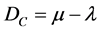(1)

where: μ is the favorable evidence degree to proposition P,

λ is the unfavorable evidence degree to proposition P.

Through this method, the contradiction degree displayed on the PAL2v vertical axis is obtained by

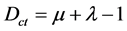(2)

The PAL2v logic is reversible and established by the following equations:

(3)

and

(4)

We can then relate the behavior and values of Paraconsistent logical states in the PAL2v Lattice, known as the Paraconsistent Universe, to evidence values that correspond to measurements in Observables of the physical world [8] - [12] .

The logical negation in PAL2v affects the certainty degree (D_C) signal and is obtained by changing evidence degrees in the annotation, such that:

(5)

when applied in the analysis of physical systems, PAL2v is called Paraquantum Logic (PQL). Therefore, the concept of Paraconsistent logical state, or Paraquantum logical state (ψ), detects a single point in the PQL Lattice formed by the pair of certainty (D_C) and contradiction (D_ct) degrees. These two values represented by a pair [8] - [12] form a single point in the PQL Lattice―a single Paraquantum logical state―represented by

(6)

A Vector of State P(ψ) in the PQL Lattice originates in one of the two vertices: True (t) or False (F), which compose the certainty degree horizontal axis. With its origin in one of the vertices of the PQL Lattice, the Vector of State P(ψ) has at its vertex a point formed by the pair indicated by the Paraquantum function [8] [12] - [17] :

.

The State Vector P(ψ) will always be the sum of its two component vectors:

Vector, with the same direction of the certainty degree axis (horizontal), whose module equals the intensity complement of the certainty degree:

Vector, with the same direction of the contradiction degree axis (vertical), whose module equals the intensity of the contradiction degree:

Given a Paraquantum logical state (ψ_cur) defined by Equation (6), we can calculate the module of Vector of State P(ψ) according to the equation:

(7)

where: = certainty degree calculated by Equation (1),

= contradiction degree calculated by Equation (2).

The angle formed by the module of the Vector of State P(ψ) and the certainty degree axis x, gives the inclination angle of the Vector of State α_ψ.

Paraquantum logical states ψ in the trajectory indicated by the vertex of State Vector P(ψ) of unitary module are defined as superposed Paraquantum logical states [8] [12] - [17] . For this one-dimensional space study, we divided the PQL Lattice into 4 quadrants.

Figure 1 shows the PQL Lattice represented by evidence degrees obtained in the physical medium and the State Vector P(ψ)_I of unitary module of quadrant I and inclination angle.

In order to advance in the study of the logical quantum model with two wave functions, a few concepts previously defined in Part I will be briefly presented.

2.1. Quantum Pulses of Concentrated Oscillation Energy

Studies on Young’s experience indicate the existence of interference phenomena beyond the two slits, in the 2W region. Quanta, or oscillation energy pulse, is thus formed by wave interference phenomena [1] [18] [19] occurring in the 2W region. For the first type of interference phenomenon, classified as Type I, we consider two waves traveling in the same direction, at the same frequency and wavelength, and at the same amplitude

but with a lag. For the second type of interference phenomenon, classified as Type II, we consider the interaction between two waves propagating in opposite directions.

The incidence of wave pulse on the two slits instantly reflects on the dynamic behavior of the waves in the 2W region. As a result, the two types of wave interference phenomenon occur simultaneously. The extraction equation of the favorable evidence degree is thus given by the following wave function equation:

(8)

With as the lag angle between two propagating waves.

Comparing Equation (3) to Equation (8), we find the wave function for the unfavorable evidence degree:

(9)

By comparing Equation (3) and Equation (4) to Equation (8) and Equation (9), we analyze wave functions that characterize the quantum in the 2W region. Therefore, the certainty degree involving its characteristic wave equation is

(10)

Likewise, the contradiction degree involving its characteristic wave equation is

(11)

After obtaining wave functions that represent evidence degrees obtained in the physical environment, in the 2W region, we can study the behavior of the quantum through the PQL Lattice [8] [12] - [17] .

In the PQL Lattice, the inclination angle of a State Vector P(ψ) of unitary module can be defined by wave functions characteristic of the quantum. By comparing the lag angle of waves in the physical environment (2W region) to the inclination angle of State Vector P(ψ) of unitary module, we observe that:

(12)

Based on these considerations, the tangent of the inclination angle of Vector of State P(ψ) is calculated with the complement value, which expresses the certainty degree:

(13)

Certainty degrees as a function of the inclination angle of the state vector P(ψ) of unitary module are expressed by the complement given by:

(14)

Similarly, contradiction degrees as a function of inclination angle of the State Vector P(ψ) of unitary module in the PQL Lattice are expressed as

(15)

According to Equation (8) and Equation (9), the certainty degree can satisfy the condition by factoring the inclination angle of the State Vector P(ψ) of unitary module into evidence degrees equations. These can be written as

(16)

(17)

Thus, each pair of evidence degrees defined by wave equations of the quantum in the 2W region corresponds to one of the superposed logical states ψ_su found in its trajectory at the vertex of the State Vector P(ψ) of unitary module in the PQL Lattice.

2.2. Complete Model for PQL-Based Quantum

For a complete one dimensional space model, we must consider that a particle, or quantum has its inflationary expansion represented in four directions (up, down, right, left) on the geometric plane. This complete geometric representation generates identical pulses for both directions of the slits in the double slit experiment. As a result, two additional 2W regions will be formed where Type I and Type II Interference phenomena occur simultaneously. Figure 2 shows this condition where the two 2W regions are

divided, thus forming evidence degrees for the correlation with the four quadrants in the PQL Lattice.

With the representation of the PQL Lattice in complex numbers, contradiction degrees, which are arranged along the vertical axis, will be represented by imaginary numbers (i); and certainty degrees, which are arranged along the horizontal axis, will be represented by real numbers.

Any Paraquantum logical state ψ located in Quadrant I of the PQL Lattice is represented by the complex number:

(18)

Through Equation (5), we can obtain the Logic negation of a Paraquantum logical state in Quadrant I, such that it will be located in Quadrant II:

(19)

The complex conjugate operator can be introduced in the Paraquantum Logical Model. Therefore, for a Paraquantum logical state in Quadrant I, its conjugated complex will be, located in Quadrant IV.

The Vector of State P(ψ)_I in Quadrant I has its intensity components on the horizontal axis and on the vertical axis, and its module will be given by:

(20)

With: and

The norm is

Following the same reasoning, the representation of complex numbers of the logical state on the Vector of State P(ψ)_IV vertex, in Quadrant IV, is given by its conjugated complex:

(21)

Using Dirac’s notation [20] combined with a nomenclature closer to that of quantum mechanics [21] [22] , we can consider for the four state vectors:

is the logical state on the vertex of the State Vector P(ψ)_I of unitary module, called Ket.

is the logic state on the vertex of the Vector P(ψ)_IV of unitary module, called Bra.

is the logical state on the vertex of the State Vector P(ψ)_II of unitary module, called ⌐Ket.

is the logical state on the vertex of the State Vector P(ψ)_III of unitary module, called ⌐Bra.

Figure 3 shows triangles in all four quadrants of the PQL Lattice and the Paraquan- tum logical states at the vertices of the four Vectors of State correlated to the 2W region through the two wave equations.

In a full model, the two information sources that appear simultaneously and with identical characteristics will create four modular State vectors P(ψ) in the PQL Lattice. In this study, we will initially highlight the Vector of State P(ψ)_I in Quadrant I, which is

characterized by a positive certainty degree of variation, and a positive contradiction degree of variation.

Vector of State P(ψ)_I moves around the origin of a True (t) logical state. This is described by 2 functions, the certainty degree function in Equation (19) and the contrad-

iction degree function in Equation (20), with inclination angle gradient of.

Given the equality in Equation (12), the lag angle ϕ of waves in 2W region will vary from 0 to π/2. Due to the unitary module of State Vector P(ψ), their vector components have amplitudes constrained to the maximum values of Certainty (D_C) and Contradiction (D_ct) Degrees. As the values depend on the lag angle ϕ of the two wave functions, consequently they also depend on the inclination angle α_ψ. From the variation of α_ψ, we will have variations for D_C and D_ct. Thus,

the horizontal component, which is related to the certainty degree, will vary, and the vertical component, which is related to the contradiction degree, will vary.

The increase of frequency f for wave functions implies a decreased in lag angle ϕ and, consequently, the maximum inclination angle α_ψmax of State Vectors will be lower than the fundamental’s angle. This increase in frequency of wave functions causes State Vectors to vibrate closer to the equidistant vertex point of PQL Lattice―the Undefined logical state (I). Thus, the smaller the inclination angle α_ψmax―meaning, the closer the state vector P(ψ) vertex is to the Undefined Logical state I represented in the PQL Lattice―the greater energy E―however, the lower its definition represented by the lowest certainty degree (D_C). Therefore, we can relate energy E and momentum M by the following equation:

(22)

And the relationship between Momentum and certainty degree is given by:

(23)

3. Energy Levels Represented by the Paraquantum Logical Model

The Paraquantum Logical Model has two Quantum-characteristic wave functions. Depending on the lag angle ϕ, functions establish a corresponding logical state in the PQL Lattice. Lag angle ϕ is represented in the PQL Lattice by the inclination angle α_ψ of the State Vector P(ψ) of unitary module. The Paraquantum logical state ψ(x, t) is represented in the lattice of the PQL at the vertex of the State Vector P(ψ) of unitary module. This will establish a trajectory with the gradient of the inclination angle α_ψ, which varies within certain limits of both components: certainty degrees (D_C) on the horizontal axis; and contradiction degree (D_ct) on the vertical axis.

The Equation for Determining Energy Levels

In the complete Paraquantum Model of one spatial dimension, the two simultaneous and identical information sources will create four State Vectors P(ψ) of unitary module in the PQL Lattice. This study highlights the State vector P(ψ)_I in Quadrant I, characterized by a positive certainty degree of variation, and a positive contradiction degree of variation.

Consider the representation of State vector P(ψ)_I, as shown in Figure 4, which indicates a Paraquantum logical state ψ located on the trajectory and on point.

A mathematical analysis is conducted in Figure 4 to determine the level of contradiction degree for each logical state ψ.

Firstly, the trajectory of the State vector P(ψ)_I vertex can be described by a circle of unitary radius around a True (t) logic state. In the PQL Lattice, contradiction degree values are on the vertical axis (y) and certainty degree on the horizontal axis (x). Therefore, any point on the circle is given by:. Line r is drawn tangentially to the trajectory of contradiction degrees’ vertical axis, in point B, where the Paraquantum logical state is located.

As shown in Figure 4, point B, for a certain wave number K and location x, can be represented by:.

In relation to the inclination angle α_ψ of the Vector of State P(ψ)_I, we have vertical and horizontal components.

Point B, where tangent line r meets contradiction degree’s vertical axis, establishes the intensity of the Paraquantum logical through the contradiction degree and can be found by the analysis shown below.

The circle equation, with its origin on the right corner of the PQL Lattice representing the True (t) logic state, is given by:.

Given that the radius and the state vector P(ψ)_I module coincide, R = 1 and the circle’s equation is given by:. For the components of the State Vector P(ψ)_I of unitary module, the circle equation is given as follows:

(24)

Equation (22) expresses values as a function of the state vector’s inclination angle α_ψ, such that:

(25)

Given any point on the circumference, the tangent line r to this point is perpendicular to the line passing through that same point and the circle’s origin.

Figure 4 shows that, in the analysis of the PQL Lattice, the point defining the tangent line r is a Paraquantum logical state, with the Vector of State P(ψ)_I defined by its components, such that:. Moreover, the angular coefficient of tangent line r is given by the derivative of the function at point.

Deriving the circle’s Equation (24) in relation to x, we have:

which is expressed by.

As a result, the angular coefficient of tangent line r that passes through the Para- quantum logical state in relation to axis x, is given by

(26)

With and we can write:

(27)

Equation (27) indicates that, for any variation of the inclination angle of the state vector P(ψ)_I―in this case varies from 0 to―the derivative of contradiction degree (on axis y) in relation to the complement of the certainty degree (on axis x) is equal to the angular coefficient m₁ of tangent liner that passes through the point defined as the Paraquantum logical state.

The equation of tangent line r is given by; with certainty and

contradiction degrees, we have:. As B is the linear coef-

ficient of tangent line r, its value corresponds, in Figure 4, to the point where tangent line r meets the contradiction degrees axis. Isolating B in the equation above, we have:

, which considering the functions’ values becomes:

(28)

We can consider B as the Paraquantum logical state intensity, which tangent line r crosses, and expressed by the contradiction degrees through PQL equations. B is, thus, the contradiction intensity standard value, obtained by the equation:

(29)

With: as the standard intensity associated to the Paraquantum logical state energy determined by the lag angles of quantum wave functions.

The function value related to the vertical component of the modular State vector P(ψ) at point A is. is the maximum inclination angle of Vector of State P(ψ)_I for the Paraquantum state to remain within the PQL Lattice. Applying Equation (29) under this assumption:

,

where we find:.

In Part I of this work, the same value was found by a different method and is connected to quantum leaps in relation to certain wave function frequencies in the 2W region.

The intensity of the contradiction degree associated to the energy of Paraquantum logical state is equal to, which is called the Paraquantum Logical Factor h_ψ. This value can be related Planck’s constant, as shown in [14] and [15] .

By locating the quantumenergy values along the contradiction degree axis of the PQL Lattice, we obtain the delta between their intensities, which is related to the tangent line r passing through this Paraquantum logical state.

As is seen in Figure 4, point B is the linear coefficient of the tangent line and indicates the intensity of the contradiction degree to which energy is attached.

At point A, the intensity of the contradiction degree equals that of the State vector P(ψ)I vertical component, which has the Paraquantum logical state ψ at its vertex crossed by tangent line r. Therefore, for point A, Intensity is related to the energy represented by the contradiction degree.

The delta between contradiction degrees is equal to the difference of corresponding Energies and is given by, where the contradiction degree intensity at point B is expressed by Equation (29). Therefore, one can obtain an equation to calculate the intensity delta of contradiction degrees. The difference between normalized energy levels results in:

(30)

For the inclination angle of State Vector P(ψ)_I at its maximum value, the difference between the intensities of the contradiction degree is given by:

A decrease in the inclination angle of State Vector P(ψ)_I below will reduce the intensity of the contradiction degree from to zero. In this variation we observe the occurrence of infinite superposed logical states. For inclination angle, intensity values would be identical and null. Therefore, the difference between their intensities would also be null. In contrast, an increase in the inclination angle of State Vector P(ψ)_I above will lead to the appearance of logical states that are not allowed by the Paraquantum Logical Model, given that they would be located outside the PQL Lattice. In the Paraquantum Model, , obtained by Equation (30), is associated to the energy potential of Schrödinger’s Equation [23] .

4. Schrödinger’s Equation in Paraquantum Analysis

To relate Schrödinger’s equation to PQL representation based on Young’s experiment (Double Slit), it is initially assumed that the energy intensity related to the quantum in the 2W region has two Observable measurements in the physical environment [1] .

These two Observables are analyzed together, with their values conforming to the principles of indeterminacy. This returns a Paraquantum logical state ψ located in the PQL Lattice, represented in the vertex of the state vector P(ψ) of unitary module. This paper considers a non-relativistic analysis that begins by relating the energy levels in Schrodinger’s equation in the PQL Lattice to values of Contradiction and certainty degrees.

4.1. Time-Independent Schrödinger’s Equation

For stationary states in quantum mechanics, Schrödinger’s equation is solved for obtaining a wave function at a given potential. Schrödinger’s Equation [17] [23] is postulated as a differential type:

(31)

where is Planck’s standard constant, m the particle mass, and V the potential involved.

This differential equation can be solved by the variable separation method, thus through product solution of simple equations that can be represented by:

where: is a function only for x, and a function only for t.

For separable solutions we have: and

Equation (31) thus becomes:

(32)

Dividing Equation (32) by, we have:

(33)

With the right side being a function only of t and the left only of x², the equality can only be real if both sides are truly constant. If this premise is false, then t variation (right side) could modify the equality’s other side (left side) without variations in x―or the two sides would no longer be equal. Based on these considerations, each side is matched to a separation constant called E.

The first equation refers to the equality’s right side of Equation (33): or

(34)

which is a common differential equation solved by:

(35)

Equation (35) can be written as

(36)

Since the angular frequency is the energy divided by Planck’s constant, then:

(37)

The second equation refers to the equality’s left side of Equation (33):

(38)

Or

(39)

Equation (39) is known as the time-independent Schrödinger’s equation whose resolution requires a potential V to be specified.

4.2. Representation of Schrödinger’s Equation in the PQL

For an analysis that allows the representation of Schrödinger’s equation in the PQL Lattice, we initially relate it [17] [23] to the Paraquantum Logical equations (PQL) [8] [15] [17] .

4.2.1. Relation between Schrödinger’s Equation and PQL Equations

In Figure 4 we observe that the analysis will be considered through the circumference’s equation as represented by the trajectories of Paraquantum logical states, which occur at the vertex of State Vector P(ψ)_I of unitary module.

4.2.2. Analysis of the Particle Equation under the Influence of Potential V

As in the Lattice of the PQL the vertical axis y represents the Contradiction Degrees, in the circumference represented representation in Figure 4, the angular coefficient m₁ of the tangent line r in relation to x, in Equation (24), can be expressed by:

.

Hence, the angular coefficient m₁ of the tangent line r in relation to x, in terms of the derivative of the contradiction degree function is

(40)

Applying the first derivative to x in the function of Equation (40), we have:

Applying the second derivative to x in the function of Equation (40), we have:

Solving only the right side of the contradiction degree function, we obtain:

(41)

Rearranging, we have:

(42)

We can make an analogy between Mechanics and (Hamilton) Optics, in which we

include a refractive index and wave number, obtaining K as subdivision is made afterwards, such that:.

, results in the equation for K squared:

Its application to Equation (40) results in:

Multiplying the denominator and divider by twice the mass m, Energy is entered by:

Finally, the entire equation is multiplied by, such that:

Thus resulting in:

(43)

A comparison between Equation (43) and Equation (39) shows that this is Schrödinger’s equation, time-independent, represented through PQL concepts. It proves that the wave function ψ of Schrödinger’s equation equals the contradiction degree function, which is exposed on the vertical axis of the PQL Lattice.

The contradiction degree function constitutes the axis of imaginary numbers in the complex numbers realm. The result of Equation (43) is thus a complex number represented by:

(44)

The second derivative of the function in relation to x is given by:

(45)

4.2.3. Analysis of the Free Particle Equation

For the ratio, where p is the particle’s momentum and is reduced Planck constant, Equation (39) can be written as

Multiplying factor by 2 times the mass m, both in the numerator and denominator, the equality corresponding to energy E can be separated:.

The equation thus becomes, from which we obtain:

(46)

Equation (46) is Schrödinger’s equation for free particles, which means, Equation (45) with potential V zeroed. In this case, the Paraquantum Logical Model represented by complex numbers indicates a wave function with values exposed in the vertical axis of the PQL Lattice. The result, which is a Contradiction degree function, is in the set of

complex numbers and can be written as. Solving

the equation’s second derivative, we have:

. Or, by Equation (45), without potential V:

(47)

4.2.4. Determination of Normalized k

The wave number K is obtained by applying the derivative of x only in the function of the contradiction degree in Equation (40), where:

(48)

Equating the result to Equation (26) or Equation (27) we have:

Suiting the signs:

From where we obtain K with normalized values through the PQL Lattice, as

(49)

For example, Equation (49) gives us K for the State vector P(ψ)_I maximum inclination angle:

With the Paraquantum logical factor, K can be written as or. Therefore, for K squared we have:.

This value is equivalent to the normalized energy value calculated through Equation (22). The value of K, after its normalization in the Lattice of the PQL, will be used in Schrödinger’s equation represented in the PQL Lattice.

4.2.5. Planck’s Constant h and the Reduced Paraquantum Logical Factor h_ψ

The intensity of contradiction degrees will shape both Planck’s units for the PQL Lattice as well as its relation to Schrödinger’s equation. Therefore, for the PQL Lattice analysis, it is possible to verify the value of its approximate value to the equivalent Paraquantum Logical factor h_ψ, such that.

For a Planck’s constant [15] - [18] equal to, its reduced value is

.

In electrovolt x seconds we have:

,

where e is the particle’s elementary charge. Assuming that the axis of contradiction degrees in the PQL Lattice is the value associated to the energy of the elementary charged particle, the corresponding electrovolt x seconds value of the Paraquantum Logical factor h_ψ is thus obtained:

derives its normalized value which, converted to elec- trovoltx seconds by

,

we find the equivalent of Planck’s reduced constant in the PQL Model as

.

And the relation between and is given by:

.

Therefore, the value of can be found from the value of, such that:

and.

4.3. Schrödinger’s Equation Represented in the PQL Lattice

For the analysis that allows the representation of Schrödinger’s equation in the PQL Lattice, we will consider the equation in Quadrant I and the circumference represented in the trajectories of Paraquantum logical states, as previously shown in Figure 4.

4.3.1. Representation Using a Time-Independent Schrödinger’s Equation

To represent Schrödinger’s equation as time-independent [17] [23] in the Lattice of the PQL, we will begin our analysis by taking Equation (43) as a reference, such that:

Since all terms are related to the sine of the inclination angle of the modular State vector P(ψ)_I, all values may be referenced to the axis of imaginary numbers in the PQL Lattice. This relation is given by:

(50)

Relating the energy intensity of Equation (39) to the term containing the Para- quantum logical factor h_ψ, we have:. Thus, we can write the contra-

diction degree in point B of Figure 4 as.

Because contradiction degree represents energy, can be considered the potential involving the energy differences in Schrödinger’s equation. Potential V of the energy difference in Schrödinger’s equation can thus be obtained in Paraquantum analysis and represented in the PQL Lattice. For this, consider Equation (30) to calculate the of intensity differences so that. Equation (50) establishes the energy values through the contradiction degrees axis, and is described as

(51)

In Figure 5 we observe the terms of Equation (50) and their equivalent intensities along the axis of contradiction degrees, where standard values are referenced by relating the energy levels obtained by the PQL to those of quantum mechanics.

For the maximum inclination angle of State Vector P(ψ)_I, Equation (51) will be equal to:

Given that:, and, thus, for this condition:

and

®

For an inclination angle and a particle under 0 potential, Equation (47) can be represented in the PQL Lattice. Therefore,

Given that:, and; thus, for this condition:

and

4.3.2. Representation Using a Time-Dependent Schrödinger’s Equation

For representing a time-dependent Schrödinger’s equation, we must initially study the condition shown in Figure 6, where Vector of State P(ψ) has a certain inclination angle α_ψ.

In the contradiction degrees’ axis for the condition shown in Figure 6, we observe that:

(52)

h₂ is the line segment above the unitary gain State Vector P(ψ). It is, thus, the hypotenuse of the right triangle, therefore:

(53)

where:

(54)

Turning Equation (54) into Equation (53) we have:

(55)

Or:

(56)

In complex numbers:

(57)

For the total energy along the contradiction degree axis, Equation (51) becomes:

(58)

where:

Or also:

In Figure 6 we observe that the angular coefficient of line r₂ that crosses over the state vector P(ψ) of unitary module is given by:

(59)

The angular coefficient of straight line r₂ is given by the derivative of function in relation to time t:

(60)

(61)

Making:

Hence:

(62)

Figure 7 shows values extracted from Schrödinger’s equation represented along the axis of Contraction Degrees of the PQL Lattice.

It’s shown that once the inclination angle of the modular state vector reaches its maximum, equals. Through Equation (60) we can calculate wi, such that:

,

and, which results in and.

The equations show that in Paraquantum analysis, Schrödinger’s equation can be studied and represented in the PQL Lattice by Contradiction (D_ct) and Certainty (D_C) Degrees. The latter are related to two wave functions, which are representatives of the quantum in the physical world.

5. Probabilistic Analysis in the Paraquantum Logic Model through Bonferroni’s Inequalities

A comparative analysis between values obtained by Schrödinger’s equation [17] [23] and those found by Paraquantum analysis allows a new approach to the discussion of

results obtained in the PQL lattice. Such considerations shall be based in values corresponding to the physical world, obtained by the two equations of wave functions characteristic of the quantum, linked to factors that can be expressed by Schrödinger’s equation. With this approach we can conduct studies on the quantum energy levels and compare results obtained with those found by Schrödinger’s equation while expanding these concepts to probabilistic analyzes, shown as follows.

Max Born’s investigations [2] [9] in quantum mechanics stood out for their statistical interpretation of the wave function and rules’ usage for probabilistic calculation [10] . We now present a probabilistic interpretation in the PQL lattice through Bonferroni Inequality [10] [11] .

5.1. Fundamental Concepts of Probabilistic Analysis

We start by presenting some fundamental concepts used in probability theory [10] .

5.1.1. Basic Notions of Probability

When an experiment is performed, the realization of the experiment is an outcome in the sample space. If the experiment is performed a number of times, different outcomes may occur each time or some outcomes may repeat. The frequency of occurrence of an outcome can be thought of as a probability, in which more probable outcomes occur more frequently. If the outcome of an experiment can be described probabilistically, we can analyze the experiment statistically.

5.1.2. Axiomatic Foundations

Definition 1.1. A set of subsets of S is called a sigma algebra (or Borel field), denoted by B, if it satisfies the following three properties:

a) (the empty set is an element of B).

b) If, then (B is closed under complementation).

c) If, then (B is closed under countable unions).

Definition 1.2 Given a sample space S and an associated sigma algebra B, a probability function is a function P with domain B that satisfies:

1) for all

2)

3) If are pairwise disjoint, then

The three properties given in the above definition are usually referred to as the Axioms of Probability or the Kolmogorov Axioms. Any function P that satisfies the Axioms of Probability is called a probability function. The following gives a common method for defining a legitimate probability function.

5.1.3. The Calculus of Probabilities

Theorem 1: If P is a probability function and A is any set in B, then;

a), where is an empty set.

b).

c)

Theorem 2: If P is a probability function and A and B are sets in B, then;

a)

b)

c) If then

5.2. Bonferroni’s Inequality and the Paraquantum Logical Model

In theorem 2, formula (b) shows an inequality which may be useful for the probability of an intersection. Given that, we have a particular inequality case, known as the Bonferroni Inequality [10] [11] :

(63)

This equation translates the relationship between values of Bonferroni’s inequality and the Paraquantum Logical Model. Therefore, in the Paraquantum analysis of Equation (63) and considering the origin of item b of Theorem 2, we have the following relationships:

↔ is associated with the favorable evidence degree given by Equation (16) and the Probability of event A.

↔ is associated with the unfavorable evidence degree given by Equation (17) and the Probability of event B.

The contradiction degree is associated with the Paraquantum Probability of an event A related to the vertical axis of the PQL Lattice:

(64)

where:

The certainty degree is associated with the Paraquantum Probability of an event A related to the horizontal axis of the PQL Lattice:

(65)

where:

The complement of the certainty degree is associated with the Paraquantum Probability of nonoccurrence of an event A related to the horizontal axis of the PQL Lattice:

(66)

Unit is associated with the State vector P(ψ) of unitary module, therefore:

(67)

We associate the complex number with the Paraquantum Probabilities and with the modular State Vector P(ψ) in Quadrant I, which establishes event’s A probability of occurrence on the vertical axis and the nonoccurrence of event A on the horizontal axis, such that:

(68)

With those considerations in mind, an increase in probability of an event A on the vertical axis decreases its probability of nonoccurrence on the horizontal axis. Conversely, as the probability of event A on the vertical axis decreases, its probability of nonoccurrence on the horizontal axis increases.

The complex value in the Paraquantum Logical Model in one spatial dimension can be determined if the quantum is in its elementary state. If so, the inclination angle of the state vector P(ψ) is maximum and we have: and. Through Equation (68):

which represents the maximum Paraquantum probability of Event A.

In its fundamental state, the event associated with the vertical axis may decrease probability of occurrence of event A until it reaches zero; while the association to the horizontal axis may increase in its probability of nonoccurrence of event A, and reach 1.

Under this condition, the quantum will be in an undefined state, with the Para- quantum logical state represented by a point equidistant from the four vertices of the PQL lattice. The complex value of the Paraquantum Logical Model in one spatial dimension can be determined if the quantum is in Undefined state.

If so, the inclination angle of the State Vector P(ψ) of unitary module is maximum, and we have: and. Through Equation (68):

which represents the minimum Paraquantum probability of Event A.

In Figure 8 we observe the Paraquantum Probability in Quadrant I of the PQL Lattice related to Bonferroni’s inequality, and its values for the fundamental state.

Therefore, wave functions represented by evidence degrees are probability functions hereby proven by Bonferroni’s inequality.

5.3. Probability Density with Analysis in the PQL Lattice

Quantum mechanics uses an interpretation initially proposed by Max Born [3] [9] , in

which a squared norm of the wave function provides the probability density of finding a particle within a certain region, in a measured position. If represents a single particle, then is the probability of finding it within interval (x, x + dx), at time t. Because particles exist at any point on axis x, the sum of probabilities of all x values must equal 1. In contrast, a total probability of zero would deny the particle’s existence [9] [23] .

The standardized condition can be expressed by since time variation is excluded from the calculation of the absolute square of the wave function:

Thus:

Wave amplitude associated with a particle, or the probability amplitude, is called wave function and is represented by. Generally, wave function is a complex variable function and the absolute square is the probability density:

(69)

where is the complex conjugate of.

As seen previously through Bonferroni’s inequality we connect the Probability theory to PQL theory; this relation is expressed through evidence degrees that represent the two wave functions obtained through studies of the interference phenomena in the 2W region that characterize the quantum. Thus, the probability amplitude, or Paraquantum wave function, is related to the Paraquantum logical state and to the State Vector P(ψ)I of unitary module represented in the PQL Lattice.

With the Paraquantum logical state represented in a set of complex numbers, as shown by Equation (18), we have:

.

where its complex conjugate is.

As references in the PQL Lattice, we have: and, and as a reference to the origin of the State Vector P(ψ) of unitary module, its module is calculated by:

For the maximum inclination angle of the State Vector P(ψ) we have:

,

and

.

The wave function of Paraquantum probability is given by the complex number:.

Given the Conjugate Complex:

The Paraquantum probability density will be

Hence, the Elementary state is identified through Probability rules in the PQL Lattice.

5.4. Representation of Complementarity in the PQL Lattice

The representation of the two wave functions and their variation in the physical environment, related to the trajectory of vertices of the State vector P(ψ)_I of unitary module in the PQL Lattice, indicates that the Ket vector becomes a Bra vector when its vertex passes through an Undetermined logic state. Thus, it can be represented as a single vector with a inclination angle variation of 0 to π/2. Furthermore, for a better representation, we can consider that the State Vector P(ψ)_I of unitary module called Ket―represented with its origin at the vertex of the True Logical State (t) of the PQL Lattice―has a Paraquantum inclination angle given by:

(70)

where the inclination angle α_ψ of the State Vector P(ψ)_I of unitary module now has a

variation from to. Thus, when the inclination angle α_ψ of the State vector P(ψ)_I of unitary module is, the Paraquantum inclination angle will be; the Paraquantum inclination angle will be when; and for, the Paraquantum inclination angle will be.

Considering point B, at the contradiction degrees axis shown in Figure 4, as the meeting point of the axis of contradiction degrees with tangent line r, the value of the contradiction degree computed by Equation (29) may reach the unit for a maximum inclination angle. For this maximum value, the intensity difference would be null and indicate a fundamental state with minimum frequency, minimum energy and maximum probability for event A.

As shown in Figure 8, if the probability favors the occurrence of event A, or of finding the particle, the certainty degree is maximum and the probability of not finding it is null. Likewise, when the inclination angle of the modular State Vector P(ψ) reaches its lowest, is null and indicates the state of maximum frequency, maximum energy and greatest likelihood of nonoccurrence of event A. If the probability is of not finding the particle, the Certainty Degree is minimal and the probability of not finding it would be total.

With the Paraquantum inclination angle obtained through Equation (70), we can determine the amount of energy (E) represented by the complemented value of the contradiction degree in Equation (22), and the probability of event A’s occurrence, or finding the particle, as the actual contradiction degree value represented in Equation (63). Thus:

And

.

Figure 9 shows this variation, in which the contradiction degree’s intensity increases with the increase of the inclination angle of State Vector P(ψ)_I, until it reaches; and then decreases once the angle is lower than, until it reaches zero.

In the analysis of the wave function of Paraquantum probability, State Vector P(ψ)I of unitary module can be represented with its origin at the equidistant point of the vertices of the PQL Lattice, where the undefined logical state occurs. Thus, with the contradiction degree at its maximum, the quantum’s energy will be minimum, or fundamental frequency, as will the Certainty Degree’s complement,. This is the maximum probability for locating the quantum.

A reduced inclination angle α_ψ corresponds to maximum energy E and momentum M, which is symbolized by the Certainty degree. Thus, the probability of finding the particle at a given location decreases until it reaches zero. Figure 10 depicts this wave function of Paraquantum probability in the PQL-based model.

With State Vectors and inclination angles as shown in Figure 10, visualization is obtained with a method that facilitates the definition of logic states within the PQL Lattice. Formalization can then be conducted by concepts close to that of quantum mechanics, such as Hilbert space, for example. Future work may thus develop into new approaches which will consider the quantum model in PQL equated in geometric space and research the effect of their interactions on particles.

6. Conclusion

This work established the concepts and formulas based on Paraquantum Logic (PQL) fundamentals, applied to the wave-particle theory. The calculations and values found through PQL analysis factored all of Schrödinger’s equation terms, which are one of the

main equations of particle wave theory. These procedures involving PQL concepts demonstrated that values found by Schrödinger equation exist within the Paraquantum Universe, as well as wave functions in this context that define quantum mechanics theories. At the end we presented the equations for quantum energy levels based on the Paraquantum Logical Model, which demonstrated that this work’s approach allowed a comparative study between Observable measurements in the physical environment and the behavior of logic states of pulses or particles associated to with the PQL Lattice, also called Paraquantum universe. We demonstrated the probabilistic study of the particle wave theory adapted to the Paraquantum Logical Model of the quantum, in one spatial dimension, using concepts of probability theory and Bonferroni’s Inequality. Given the vastness of quantum mechanics theory, we highlighted only its main topics―those deemed crucial to the development of more detailed PQL-based concepts. They revealed that the representation of the two quantum wave functions opened a wide field for new discoveries and considerations given that the model can be applied to new developments in the field of Physics. Our next work will be to develop algorithms for quantum computing based on this Paraquantum logical model proposed. These new PQL-algorithms will cover the phenomena of symmetry and entanglement as well as other quantum phenomena, which will allow the investigation of transmission capacity of cryptographic signals based on Paraquantum Logic PQL.

Acknowledgements

We thank Newton C. A. Da Costa (PhD) who was one of the creators of Paraconsistent Logic.

We thank Crimson Interactive Pvt. Ltd. (Ulatus)―www.ulatus.com.br for their assistance in manuscript translation.

Cite this paper

Da Silva Filho, J.I. (2016) Undulatory Theory with Paraconsis- tent Logic (Part II): Schrödinger Equation and Probability Representation. Journal of Quantum Information Science, 6, 181-213. http://dx.doi.org/10.4236/jqis.2016.63013

References

- 1. Qureshi, T. (2012) Modified Two-Slit Experiments and Complementarity. Journal of Quantum Information Science, 2, 35-40.
http://dx.doi.org/10.4236/jqis.2012.22007 - 2. Barr, E.S. (1963) Men and Milestones in Optics II. Thomas Young. Applied Optics, 2, 639-647.
http://dx.doi.org/10.1364/AO.2.000639 - 3. Griffiths, D. (1995) Introduction to Quantum Mechanics. Prentice Hall, Upper Saddle River, New Jersey.
- 4. Narasimhachar, V., Poostindouz, A. and Gour, G. (2016) Uncertainty, Joint Uncertainty, and the Quantum Uncertainty Principle. New Journal of Physics, 18, Article ID: 033019.
http://dx.doi.org/10.1088/1367-2630/18/3/033019 - 5. Da Costa, N.C.A. (1974) On the Theory of Inconsistent Formal Systems Notre Dame. Journal of Formal Logic, 15, 497-510.
http://dx.doi.org/10.1305/ndjfl/1093891487 - 6. Blair, A.H. and Subrahmanian, V.S. (1987) Paraconsistent Logic Programming. 7th Conference on Foundations of Software Technology and Theoretical Computer Science, Pune, 17-19 December 1987, 340-360.
http://dx.doi.org/10.1007/3-540-18625-5_59 - 7. Da Costa, N.C.A., Subrahmanian, V.S. and Vago, C. (1991) The Paraconsistent Logic PJ. Mathematical Logic Quarterly, 37, 139-148.
http://dx.doi.org/10.1002/malq.19910370903 - 8. Da Silva Fiho, J.I., Lambert-Torres, G. and Abe, J.M. (2010) Uncertainty Treatment Using Paraconsistent Logic: Introducing Paraconsistent Artificial Neural Networks. IOS Press, Amsterdam, 328.
- 9. Born, M. (1969) Physics in My Generation. Springer-Verlag, New York.
http://dx.doi.org/10.1007/978-3-662-25189-8 - 10. Hunter, D. (1976) An Upper Bound for the Probability of a Union. Journal of Applied Probability, 13, 597-603.
http://dx.doi.org/10.1017/S0021900200104164 - 11. Galambos, J. and Simonelli, I. (1996) Bonferroni-Type Inequalities with Applications, Probability and Its Applications. Springer-Verlag, New York, x+269.
- 12. Da Silva Filho, J.I. (2011) Algorithms Based on Paraconsistent Annotated Logic for Applications in Expert Systems. In: Segura, J.M. and Reiter A.C., Eds., Expert System Software: Engineering, Advantages and Applications, Nova Science Publishers, Hauppauge, 1-40.
- 13. Da Silva Filho, J.I. (2014) An Introduction to Paraconsistent Integral Differential Calculus: With Application Examples. Applied Mathematics, 5, 949-962.
http://dx.doi.org/10.4236/am.2014.56090 - 14. Da Silva Filho, J.I. (2011) Paraconsistent Annotated Logic in Analysis of Physical Systems: Introducing the Paraquantum Factor of Quantization hψ. Journal of Modern Physics, 2, 1397-1409.
http://dx.doi.org/10.4236/jmp.2011.211172 - 15. Da Silva Filho, J.I. (2011) Analysis of Physical Systems with Paraconsistent Annotated Logic: Introducing the Paraquantum Gamma Factor γψ. Journal of Modern Physics, 2, 1455-1469.
http://dx.doi.org/10.4236/jmp.2011.212180 - 16. Da Silva Filho, J.I. (2012) Analysis of the Spectral Line Emissions of the Hydrogen Atom
with Paraquantum. Journal of Modern Physics, 3, 233-254.
http://dx.doi.org/10.4236/jmp.2012.33033 - 17. Da Silva Filho, J.I. (2012) An Introductory Study of the Hydrogen Atom with Paraquantum Logic. Journal of Modern Physics, 3, 312-333.
http://dx.doi.org/10.4236/jmp.2012.34044 - 18. Tipler, P.A. and Llewellyn, R.A. (2007) A Modern Physics. 5th Edition, W. H. Freeman and Company, New York.
- 19. Mckelvey, J.P. and Grotch, H. (1978) Physics for Science and Engineering. Harper and Row, Publisher, Inc., New York, London, 426 p.
- 20. Dirac, P.A.M. (1958) The Principles of Quantum Mechanics. 4th Edition, Oxford University Press, Oxford, UK.
- 21. Bernstein, J., Fishbane, P.M. and Gasiorowicz, S.G. (2000) Modern Physics. Prentice-Hall, Upper Saddle River, New Jersey, 624 p.
- 22. Feynman, R.P., Leighton, R.B. and Sands, M. (1965) The Feynman Lectures on Physics, Vol. 3. Addison-Wesley Publishing Company, Boston.
- 23. SchrÖdinger, E. (1926) An Undulatory Theory of the Mechanics of Atoms and Molecules. The Physical Review, 28, 1049-1070.
http://dx.doi.org/10.1103/PhysRev.28.1049