Journal of Quantum Information Science
Vol. 3 No. 4 (2013) , Article ID: 40156 , 11 pages DOI:10.4236/jqis.2013.34017
A New Way to Implement Quantum Computation
University of Cassino, Cassino, Italy
Email: gennaro.auletta@gmail.com
Copyright © 2013 Gennaro Auletta. This is an open access article distributed under the Creative Commons Attribution License, which permits unrestricted use, distribution, and reproduction in any medium, provided the original work is properly cited.
Received September 10, 2013; revised October 23, 2013; accepted November 8, 2013
Keywords: Lindenbaum-Tarski Algebra; 3D Logical Space; Mechanical Computation; Inference; Quantum Computing; Raising Operators; Lowering Operators
ABSTRACT
In this paper, I shall sketch a new way to consider a Lindenbaum-Tarski algebra as a 3D logical space in which any one (of the 256 statements) occupies a well-defined position and it is identified by a numerical ID. This allows pure mechanical computation both for generating rules and inferences. It is shown that this abstract formalism can be geometrically represented with logical spaces and subspaces allowing a vectorial representation. Finally, it shows the application to quantum computing through the example of three coupled harmonic oscillators.
1. Introduction
I shall present an expansion of the Lindenbaum-Tarski algebra into a three-dimensional logical space [1-3]. The Venn diagrams are shown in Figure 1 while the relative truth-value assignation is in Table 1. Let us compute the combinatory of this logical space, considering that we have 8 truth-value assignation and therefore statements defined through a string of 8 numbers.
A combinatorial calculus gives 9 logical levels determined by the number of 1s or 0s (where the first figure denotes the number of 1s while the second open the numbers of 0s):
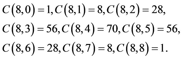
In this way, any (of the 256) statements occupy a well definite position and it is identified by a numerical ID. This allows pure mechanical computation both for generating rules and inferences. Let us therefore represent all the propositions at the different levels through Tables 2-10 (the expression  means the product of the complement sets of f and h).
2. Subspaces
A three-dimensional logical space embeds three twodimensional logical subspaces and three one-dimensional ones. A one-dimensional (1D) subspace is constituted by the following nodes: ,
,  ,
,  , and
, and . In the following, I shall use a number for each of the nodes
  and
and  and do not consider tautology and contradiction as long as we deal with subspaces (in fact, there is every time only one tautology and one contradiction for the whole space). This has the purpose to fully replace the calculus on variables with a
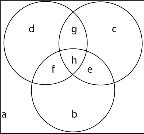
Figure 1. The Venn diagrams when the relations among three statements are considered. Note that we have: X = d + f + g + h, Y = c + e + g + h, Z = b + e + f + h.

Table 1. Inputs and outputs of 3-dimensional logic.

Table 2. C(8,8) = C(8,0).
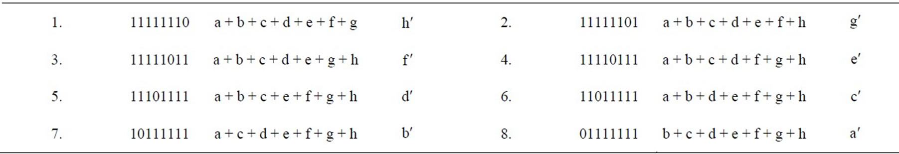
Table 3. C(8,7) = 8 disjunctive eptaplets, C(8, 1) = 8 conjunctive singlets.
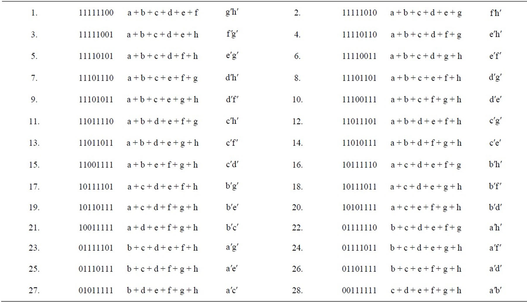
Table 4. C(8,6) = 28 disjunctive esaplets, C(8,2) = 28 conjunctive duplets.
calculus on the subspaces. Therefore, I shall assign the numbers 1 and 2 to nodes  and
and , respectively, and call each one the complement zero-dimensional (0D) space of the other. For the sake of simplicity, here and in the following I shall call also 1 or 2 simply subspaces although they are in fact nodes of a single onedimensional (1D) subspace or 0D spaces. Keeping this in mind, that widening of the term makes no problem but helps the simplification of the language. Therefore, the one-dimensional subspace can be represented as a thread connecting the nodes 1 and 2 as shown in Figure 2. Therefore, let us assign a (0D) subspace to each of the values displayed in Table 1 for each variable:
The six one-dimensional subspaces are therefore 1 - 2, 7 - 8 for , 3 - 4, 9 - 10 for
  and 5 - 6, 11 - 12 for
 . This generates three two-dimensional (2D) subspaces that are therefore embedded in the three-dimensional logical space:
As we can see in Figure 3, a single 2D space is build by creating a surface connecting the two 1D subspaces and therefore all their nodes. In order to generate all the possible three-dimensional combinations we need first to understand what means to be in a 3D space. Let us first understand what is the correct relation between subspaces and variables. For one-dimensional subspaces they obviously coincide. In this case, in fact the variable 
 is spanned by the subspace 2 (1). For the two-dimensional subspaces the same remains true, although here there is a multiplication of subspaces relative to the variables. However, as long as these 2D subspaces remain separated, the situation is not substantially different. However, in the three-dimensional space
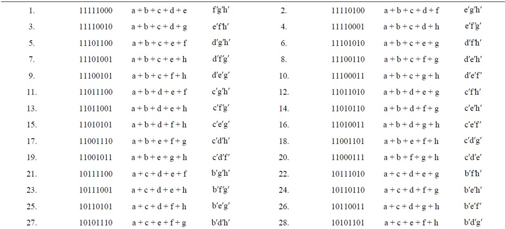
Table 5. C(8,5) = 56 disjunctive pentaplets, C(8,3) = 56 conjunctive triplets.
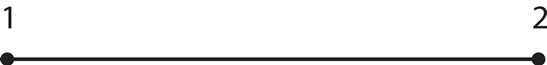
Figure 2. One-dimensional space.
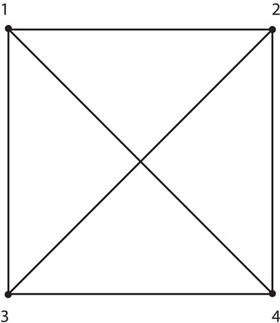
Figure 3. Two-dimensional space.
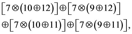
all variables and subspaces can be connected. In fact, we have e.g. that at the level 4 - 4 displayed in Table 6 we have the following combination of subspaces from below
where, when building subspaces, I shall consider the operation of sum  and product
  of these subspaces; and from above
These two expressions, somehow single out the subspace 1. However, since the subspace 1 is outside the 2D subspace represented by the intersection 9 - 11, 10 -
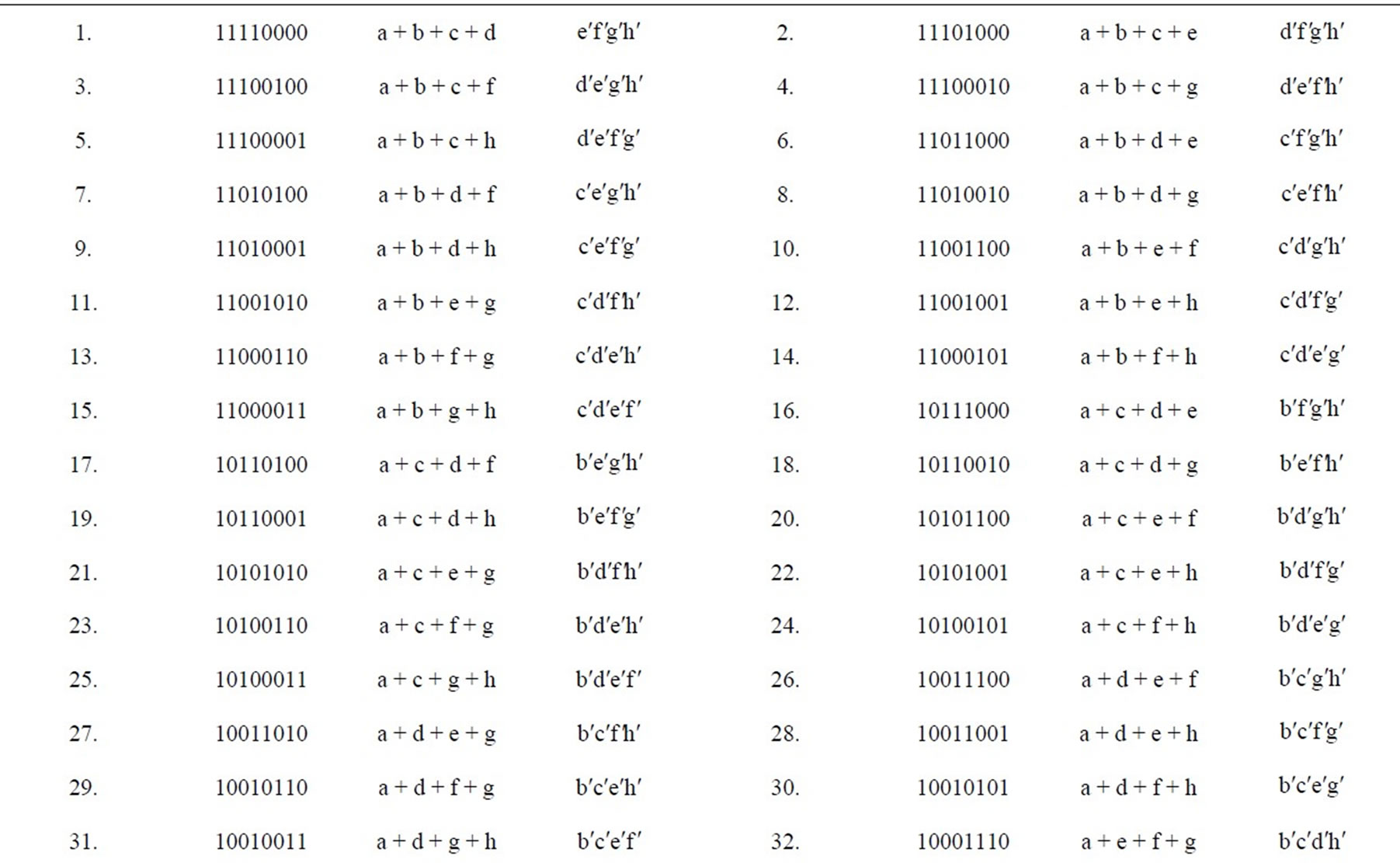
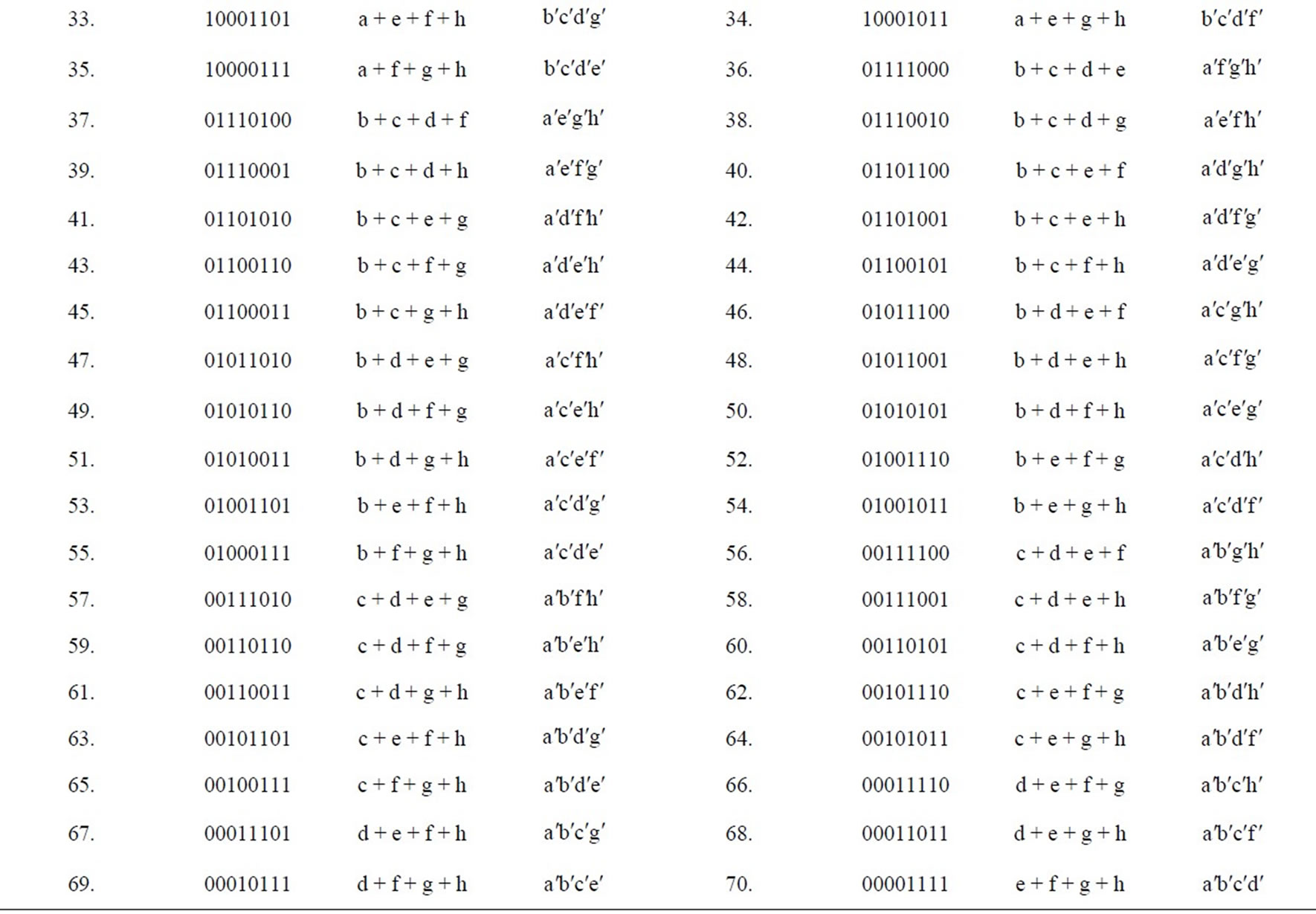
Table 6. C(8,4) = 70 disjunctive quadruplets, C(8,4) = 70 conjunctive quadruplets.
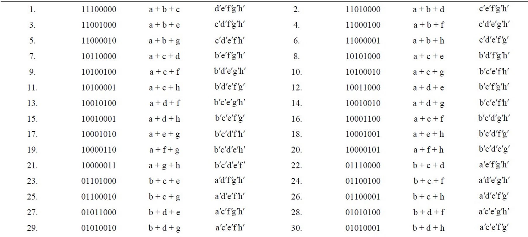
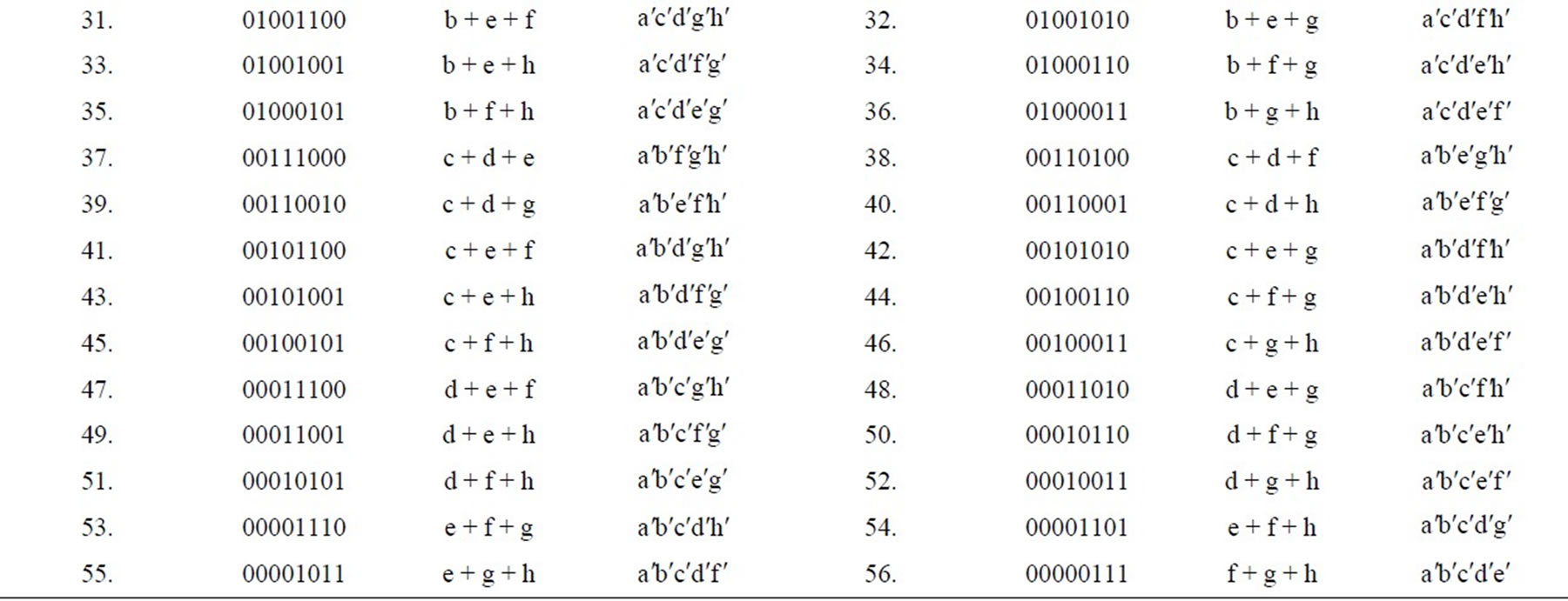
Table 7. C(8,3) = 56 disjunctive triplets, C(8,5) = 56 conjunctive pentaplets.
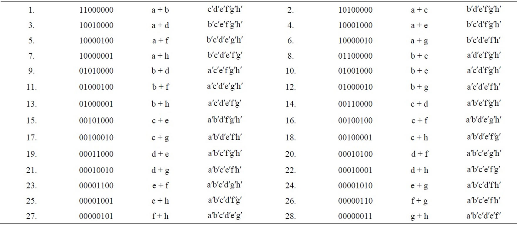
Table 8. C(8,2) = 28 disjunctive duplets, C(8,6) = 28 conjunctive esaplets.
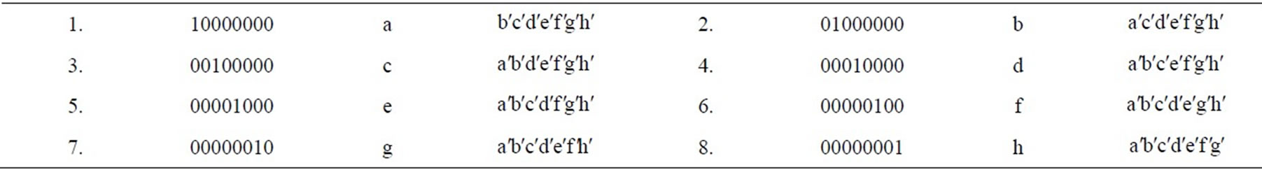
Table 9. C(8,1) = 8 disjunctive singlets, C(8,7) = 8 conjunctive eptaplets.

Table 10. C(8,0) = C(8,8).
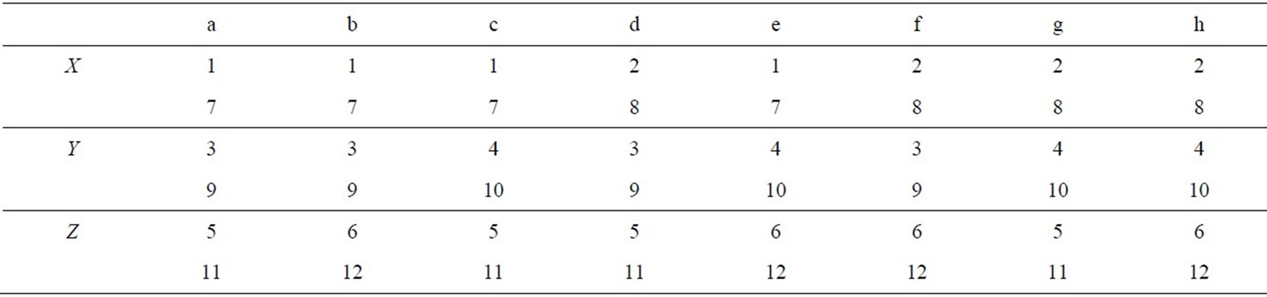
Table 11. One-dimensional subspaces in the tridimensional space.
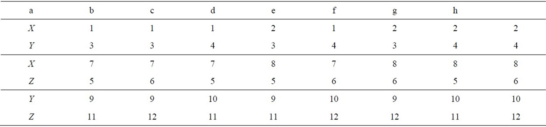
Table 12. Two-dimensional subspaces in the tridimensional space.
12, then we could also substitute 1 by 7 and write from below
and from above
This shows that both 1 and 7 point to the same variable  and therefore we can consider the variable
 to be the coincidence of these two subspaces. Let us symbolize it as
 , and similarly for the other variables. Therefore, when we deal with connections through the 3D space we always have these cross spaces. This is crucial, since in this way we are able to explicitly symbolize the range of each variable when it is taken in connection with other ones. This is what makes the use of subspaces more rigorous than those of variables and allows us both to drop any use of quantification and deal with generalized relations. Therefore, the 3D space takes the form of a pentahedron with three surfaces representing the three 2D subspaces that generate three triangles in which the three vertexes are nodes of all the three variables, as displayed in Figure 4.
From a geometrical point of view, each n-1D subspace can be seen as a projection of the nD overordined space. This allows us to make use of partial derivatives with the additional difficulty that the planes we deal with are not orthogonal.
This formalism allows in principle to treat subspaces as the main tool of logic and therefore as boxes in which we can insert some content, and the variables as “dummy” variables that can be put in those boxes according to needs of computation. Nevertheless I shall still keep the use of variables as far as it can help the reader to assimilate this new way to treat logic. I also remark that in order to ascertain how many subspaces we have for a n-dimensional logic, it suffices to multiply the number of subspaces of the n-1-dimensional logic with the number of variables of the n-dimensional logic. This makes the following series:
• 1 1D subspace (2 0D ones) for the one-dimensional logical spaceŸ  1D (4 0D) subspaces for the twodimensional logical spaceŸ
  1D (12 0D) subspaces for the threedimensional logical spaceŸ
  1D (48 0D) subspaces for the fourdimensional logical spaceŸ
  1D (240 0D) subspaces for the fivedimensional logical space, and so on.
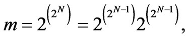
This is one of the main advantages of dealing with subspaces instead of logical expressions. In fact, whilst the number of monadic subspaces increases by a multiplication factor as the number of dimensions (variables) increases according to the formula , where
  parametrizes the subspaces and
  parametrizes the variables, the number
  of logical expressions grows exponentially as the number of variables increases:
 (1)
(1)
where again  is the number of variables.
In analogy with traditional logical expressions, the following formulae can be helpful:
 .
.
 .
.
• .
.
• .
.
 .
.
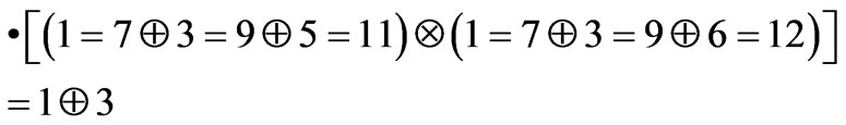
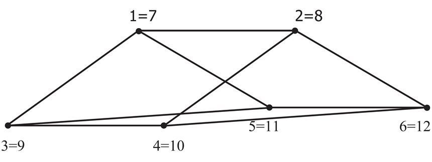
Figure 4. Three-dimensional space. Only the edges of the pentahedron are shown for the sake of representation.
These operations display the fact that the concept of subspace has certain analogies with that of logical expression. However, it is also slightly different. The last passage on the right shows only simplified connections between  and
and  since it involves only their 2D subspace.
Let us consider that the whole 3D space is constituted from a low level and an upper level instantiating formulae representing the combination of all three variables through product and sum, respectively (Levels 1 - 7 and 7 - 1as displayed in Tables 3 and 9, respectively: I do not consider here contradiction and tautology). The pairwise combination of both the first and the second kind of statements will generate binary relations in terms of product and sum (Levels 2 - 6 and 6 - 2as displayed in Tables 4 and 8, respectively), that is a piece of twodimensional logic. The pairwise combination of the first and second kind of binary relations will generate all cross triplets (Levels 3 - 5 and 5 - 3 as displayed in Tables 5 and 7, respectively). Finally, the combination of the latter two kinds of formulae will generate from above and below the same formulae (Level 4 - 4). Most of these expressions involve all three variables but some of them are also monadic expression, another piece of twodimensional logic and also the essence of one-dimensional one (Level 4-4). We may consider the expressions above for , as an example.
3. A Vectorial Representation
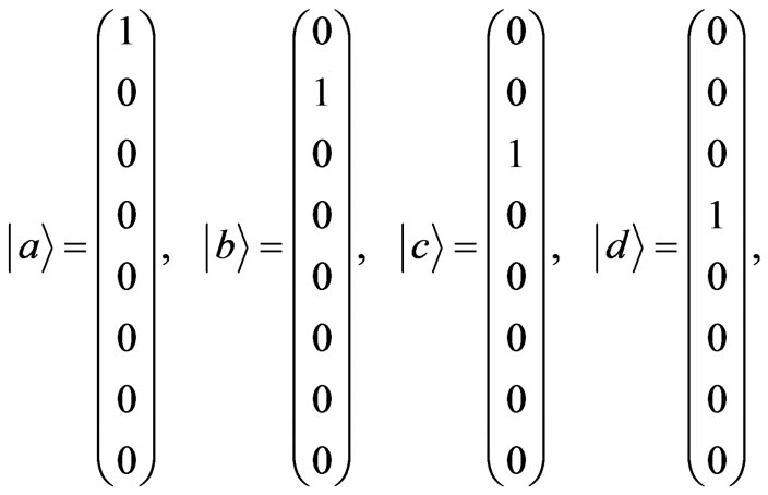
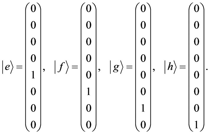
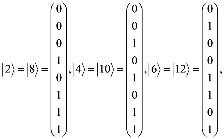
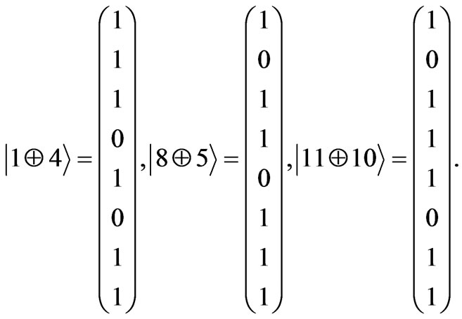
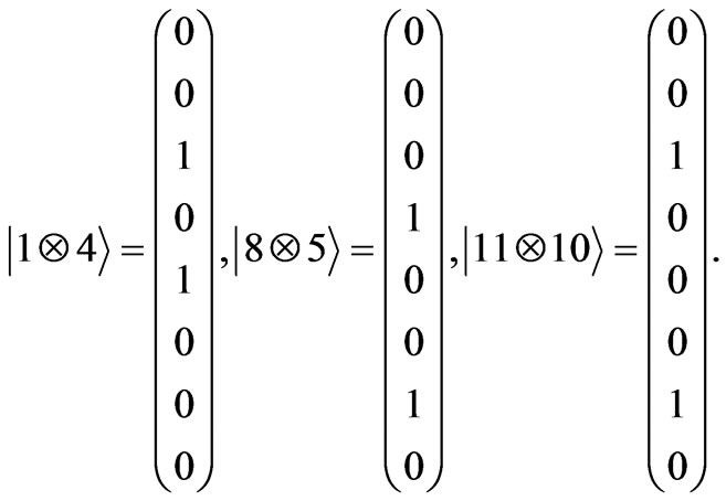
An interesting possibility is to conceive all logical statements and also subspaces in vectorial terms [4] . We can indeed represent the 8 value assignments in Tab. 1 in terms of the following orthogonal basis:
 (2)
(2)
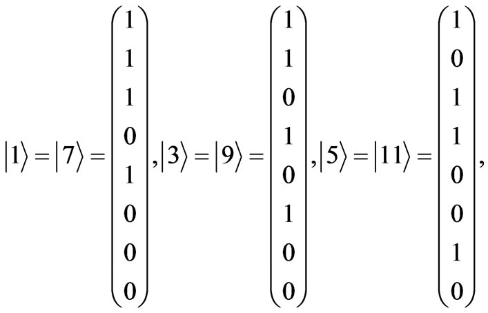
We are now in position to write any statement in the 3D space as a combination of these basis vectors. However, also the 0D components of any subspace can be written in this terms, since we have:
 (3)
(3)
where the columnar sequence of numbers corresponds to the ID of each denoted variable or statement. Note that 
 and
and 
 constitute an orthogonal basis for the 1D logical space and similarly for the other variables. Instead, all vectors on the first row are parallel (as well as those in the second row), what can be seen by the fact that they pairwise share 4 values out of 8 (2 out of the first 4 numbers and the other 2 out of the last 4 numbers of each column vector). This means that the 2D reference frame whose axes are
  and
and  is displaced of some length relative to reference frame constituted by axes
  and
and . This means that the line connecting the points individuated by
  and
and  and the line connecting the points individuated by
  and
and  are parallel, what allows to recover the plane shown in Figure 3, as displayed in Figure 5. Similarly, also the reference frame whose axes are
  and
and  is displaced of same length relative to the reference frame
 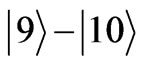 as well as the he reference frame whose axes are
  and
and  is displaced of same length relative to the reference frame
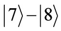 . This allows to fully recover the 3D logical space of Figure 4, as displayed in Figure 6. Note that at least one of the reference frames (here
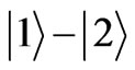 ) needs to be displaced along two directions, one for each of the other two reference frames.
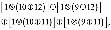
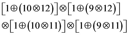
An alternative representation is to make use of 2D subspaces as vectors. For instance an orthogonal basis is constituted by subspaces
 , where
  stands for either sum or product between subspaces. If we take all these alternative choices together in the 3D space, we get an intersection of two planes as shown in Figures 7 and 8. Note that the vectors of the second representation can be considered as superpositions of the first one and vice versa.
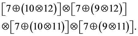
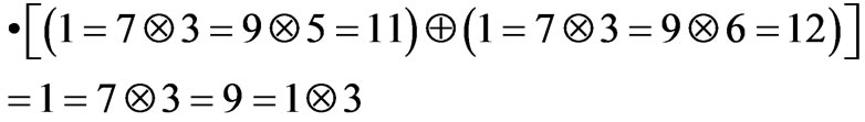
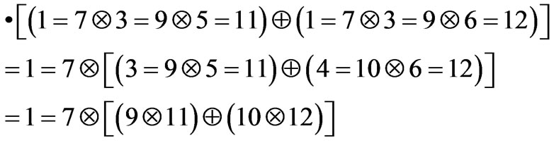
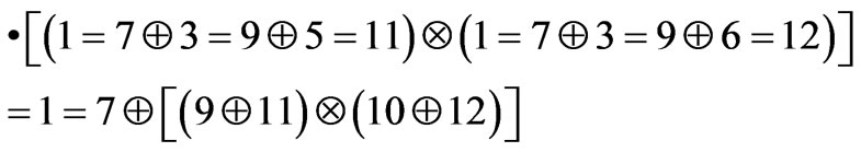
This representation allows us to write a classical derivation like the syllogism Barbara in this terms:
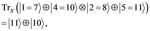 (4)
(4)
where  symbolizes the mathematical operation of tracing the “system”
  out. However, considered that
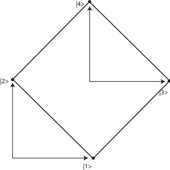
Figure 5. Relations between 2D vectorial spaces and 2D logical subspaces.
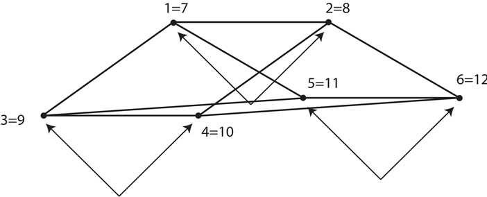
Figure 6. Relations between 3D vectorial spaces and 3D logical space.
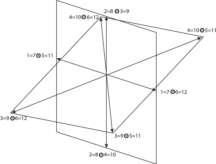
Figure 7. 2D subspaces as vectors: first two planes.
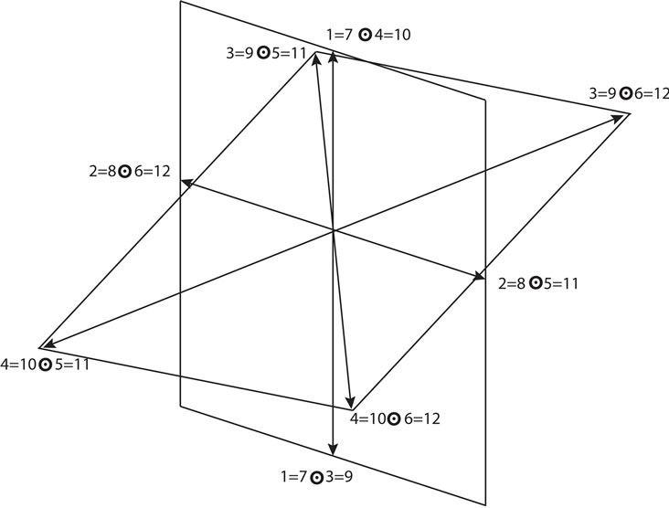
Figure 8. 2D subspaces as vectors: second two planes (the horizontal plane is only rotated relatively to the previous figure).
the nature of the connections (that have the value of operations on logical subspaces) the sign connecting (either  or
or ) the two states in the final state needs to correspond to logical rules. Such a tracing out corresponds to a kind of information election, what establishes an interesting connection between inferences and information [5]. These rules allow for following definitions:
 (5)
(5)
Analogously, we can define similar vectors in the case of subspaces product, for instance:
 (6)
(6)
Clearly, all of the above vectors represent the IDs of the relative statements.
4. Quantum Computing: Raising and Lowering Operators
The previous formalism can be easily used for implementing quantum computation [6-8; 9: Ch.17]. For instance, we can represent the three sets  and
and  as three harmonic oscillators that can be in ground (0) or excited (1) state each (it suffices to choose and arbitrary state
  as the threshold between ground and excited states; otherwise systems implementing binary choices can be chosen, for instance spin-particles). What we need then is a family of raising and lowering operators allowing us to climb or descend the ladder of the possible states. We focus on the tridimensional logic (the results can be easily extracted for the oneand bi-dimensional case). Obviously, the rules for product and sum established previously need always to be taken into account. We can build a family of raising operators whose combination can give rise to any of the passages from one level to the next higher one (see Figure 9). Any of these operators can be assumed to act on columnar vectors represented by the ID sequence of each statement of the starting level (as shown in the previous section) and produces other columnar vectors of the upper level as output (repetitions are not considered as well as results that are identical to the input).
Mathematically speaking, we cannot act with a raising operator on a vector composed only of zeros (Level 0 - 8). However, this can be easily done by adding a qubit representing the environment and keeping it constant (=1) so that it is irrelevant for the operations inside the logical space. Having said this, in the following I shall no longer deal with this problem.
A family of raising operators from Level 1 - 7 to Level 2 - 6 is shown in Figure 10. They are the result of the combination of the previously shown operators. Starting from the top line from the left to right (see Tables 8 and 9):
• The first operator allows the generation of Level 2 - 6 Statements 1, 8, 14, 19, 23, 26, and 28. Consider that the number of the propositions perfectly correspond to the number of the operator in the series displayed in Figure 9 and the same is true for each of the subsequent transformations. This is due to the fact that each of these statements is an eigenvector of this operator and the same is true for the following transformations.
• The second one the generation of Statements 2, 9, 15, 20, 24, and 27.
• The third the generation of Statements 3, 10, 16, 21, 25.
• The fourth (the first on left in the bottom line) the generation of Statements 4, 11, 17, and 22.
• The fifth the generation of Statements 5, 12, 18.
• The sixth the generation of Statements 6 and 13.
• Finally, the last operator generates Statement 7.
The raising operators allowing the ascension from
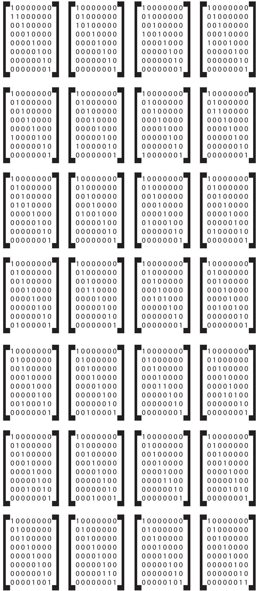
Figure 9. The 28 raising operators allowing the passage from any level to the next higher one.
Level 2 - 6 to Level 3-5 (see Tables 7 and 8) are represented in Figure 9 (always starting from the top line from the left to right):
• Operator 1 generates Level 5-3 Statements 1, 2, 3, 4, 5, 6.
• Operator 2 generates Statements 7, 8, 9, 10, 11.
• Operator 3 generates Statements 12, 13, 14, 15.
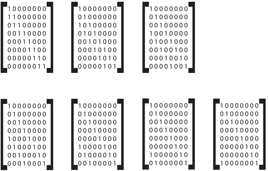
Figure 10. The seven raising operators allowing the passage from Level 1 - 7 to Level 2 - 6.
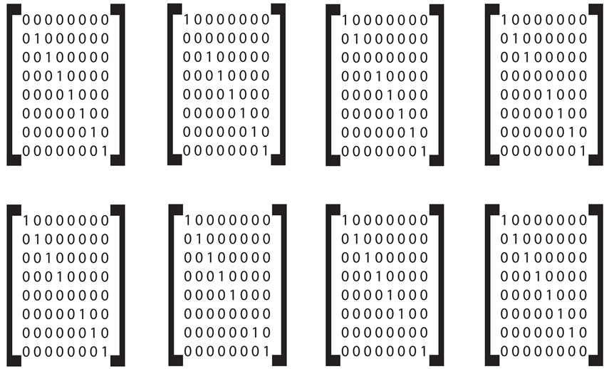
Figure 11. The eight lowering operators allowing the passage from any level to the next lower level.
• Operator 4 generates statements 16, 17, 18.
• Operator 5 generates Statements 19, 20.
• Operator 6 generates Statement 21. Operator 7 is redundant.
• Operator 8 generates Statements 22, 23, 24, 25, 26.
• Operator 9 generates Statements 27, 28, 29, 30.
• Operator 10 generates Statements 31, 32, 33.
• Operator 11 generates Statements 34 and 34.
• Operator 12 generates Statement 36. Operator 13 is redundant.
• Operator 14 generates Statements 37, 38, 39, 40.
• Operator 15 generates Statements 41, 42, 43.
• Operator 16 generates Statements 44 and 45.
• Operator 17 generates Statement 46. Operator 18 is redundant.
• Operator 19 generates Statements 47, 48, 49.
• Operator 20 generates Statements 50 and 51.
• Operator 21 generates Statement 52. Operator 22 is redundant.
• Operator 23 generates Statements 53 and 54.
• Operator 24 generates Statement 55. Operator 25 is redundant.
• Operator 26 generates Statement 56. Operators 27 and 28 are redundant.
Again I have not considered repetition, so that "later" operators are more diminished in their generating capacity than is actually the case. We can reiterate this procedure and generate any subsequent level.
The lowering operators that bring back statements from any given level to the next lower one can be built as in Figure 11. It is clear that the first one (always starting from the top line from the left to right) annihilates the term a in any statement, the second the term b, and so on. They are sort of negative projectors: instead of projecting e.g. on the component a they project on not-a.
5. Conclusion
What is interesting with the previous approach is that we can build a quantum computer that generates only logical statements (in fact any of the previous 256 statements and their connections in the 3D space are logical). This means that we can build in this way any kind of logical rule. Moreover, by implementing the procedures of tracing-out, we are able to generate any kind of inference on a quantum computer. In other words, a quantum “processor” would spontaneously generate both logical rules and inferences, which would represent a considerable progress.
REFERENCES
- G. Boole, “An Investigation of the Laws of Thought, on Which Are Founded the Mathematical Theories of Logic and Probabilities,” New York, Dover, 1958.
- A. Tarski, “On the Foundations of Boolean Algebra,” Vol. 10, 1935, pp. 320-341.
- G. Auletta, “Mechanical Logic in three-Dimensional Space,” PanStanford Pub, Peking, 2014.
- G. Auletta and S.-Y. Wang, “Quantum Mechanics for Thinkers,” Pan Stanford Pub, Peking, 2014.
- G. Auletta, “Inferences with Information,” Universal Journal of Applied computer Science and Technology, Vol. 2, No. 2, 2012, pp. 216-221.
- H.-K. Lo, S. Popescu and T. Spiller, “Introduction to Quantum Computation and Information,” World Scientific, Singapore, 1998.
- M. A. Nielsen and I. L. Chuang, “Quantum Computation and Quantum Information,” University Press, Cambridge, 2011.
- D. Bouwmeester, A. K. Ekert and A. Zeilinger, “The Physics of Quantum Information: Quantum Cryptography, Quantum Teleportation, Quantum Computation,” Springer, Berlin, 2000.
- G. Auletta, M. Fortunato and G. Parisi, “Quantum Mechanics,” University Press, Cambridge, 2009.
- A. Tarski, Logic, “Semantics, Meta-Mathematics,” University Press, Oxford, 1956.