Open Journal of Statistics
Vol.06 No.04(2016), Article ID:69318,25 pages
10.4236/ojs.2016.64048
Markov-Switching Time-Varying Copula Modeling of Dependence Structure between Oil and GCC Stock Markets
Heni Boubaker*, Nadia Sghaier
IPAG LAB, IPAG Business School, Paris, France

Copyright © 2016 by authors and Scientific Research Publishing Inc.
This work is licensed under the Creative Commons Attribution International License (CC BY).
http://creativecommons.org/licenses/by/4.0/


Received 26 May 2016; accepted 26 July 2016; published 29 July 2016
ABSTRACT
This paper proposes a Markov-switching copula model to examine the presence of regime change in the time-varying dependence structure between oil price changes and stock market returns in six GCC countries. The marginal distributions are assumed to follow a long-memory model while the copula parameters are supposed to evolve according to the Markov-switching process. Furthermore, we estimate the Value-at-Risk (VaR) based on the proposed approach. The empirical results provide evidence of three regime changes, representing pre-crisis, financial crisis and post-crisis, in the dependence structure between energy and GCC stock markets. In particular, in the pre- and post-crisis regimes, there is no dependence, while in the crisis regime, there is significant tail dependence. For OPEC countries, we find lower tail dependence whereas in non-OPEC countries, we see upper tail dependence. VaR experiments show that the Markov-switching time- varying copula model performs better than the time-varying copula model.
Keywords:
Time-Varying Copulas, Markov-Switching Model, Oil Price Changes, GCC Stock Markets, VaR

1. Introduction
It is widely recognized that the energy and stock markets are very closely tied. Theoretically, changes in the oil price are the most significant factor influencing the returns of stock market indices, either directly by affecting the future cash flows or indirectly through impacting the interest rate considered to discount the future cash flows.
Regarding the Gulf Cooperation Council (GCC) countries1, numerous empirical studies have been developed to examine the linkages between oil price changes and stock market returns using various econometric approa- ches. Previous studies rely on linear times series models like VAR and VAR-GARCH to study short-term dynamics [1] - [5] ; while other studies adopt linear cointegration techniques to test for a stable long-term rela- tionship between oil prices and stock market indices [6] - [8] .
An important precondition for the validation of the linear models is the stability of the models and the invariability of the parameters over time. In practice, this assumption is far from being satisfied due to the pre- sence of structural breaks [9] and regime change [10] . Consequently, the parameters are time-varying and the model seems to be non-linear.
The evidence of non-linearity of the relationship between oil price changes and GCC stock market returns has been provided by [11] for the case of Bahrain, Kuwait and Saudi Arabia and by [12] for Oman, Qatar and the UAE, but not for Bahrain, Kuwait or Saudi Arabia. Applying panel data with regime-shift techniques, [13] validates a non-linear long-run relationship between GCC stock market indices and three global factors in- cluding the oil price, the MSCI World index and the US one-month Treasury bill interest rate. Using the Markov-switching model, [14] find evidence of three regimes (low, high and crash volatility) on the relationship between oil price changes and stock market returns.
It is well-known that these models are limited because they do not allow for the asymmetric effect of increases and decreases in oil prices on stock markets returns. In this sense, some studies show that the stock markets are more sensitive to negative oil shocks than to positive oil shocks [15] - [17] . To reproduce this asymmetric effect in GCC countries, [18] introduce a dummy variable2 in the linear model and find that the decreases in oil prices have a significant negative impact on stock market returns, whereas the increases in oil prices present a strong positive effect on the stock market returns in Saudi Arabia and the UAE only. [19] employ a DCC-GARCH model and show that the correlation between stock market returns and oil price changes varies over time.
Although the DCC-GARCH model allows for the time-varying conditional correlation, it fails to reproduce the non-linear dependence that may exist between the variables and does not provide information about the tail dependence. The tail dependence corresponds to the possibility of joint events such as low or high extreme event occurrence. To do so, an alternative approach based on copula functions has been adopted. The main advantage of the copulas lies in separating the dependence structure from the marginals without making any assumptions about the distribution. Using several copula functions, [20] provide evidence of left tail dependence in Vietnam, whereas there is no tail dependence in China. For the case of six CEE countries (Bulgaria, Czech Republic, Hungary, Poland, Romania and Slovenia), [21] also find left tail dependence.
The main insufficiency of these copula functions is that the dependence structure is supposed to be constant over time. To allow for variability in the dependence structure, [22] develops the time-varying copula functions that suppose that the copula parameter evolves according the ARMA model. The time-varying copula functions have been adopted by [23] and [24] to examine the dynamic dependence structure between oil price changes and stock market returns in US/China and ten Asia-Pacific countries respectively. Though this approach permits for variability in the dependence structure, it assumes that the copula parameter evolves linearly and does not provide information about the change in the copula parameter.
More recent studies show that the financial crisis has a considerable impact on the dependence structure between oil price changes and stock market returns. For instance, [25] analyze the dependence structure between oil price changes and macroeconomic variables using Archimedean copulas in six GCC countries. They find that the dependence structures between the series differ in each country. In addition, they divide the period into two sub-periods: tranquil period and crisis period to check whether the dependence structure is affected by the financial crisis. They find different dependence structures: Before the financial crisis, they provide evidence of symmetric dependence, but after financial crisis they provide evidence of asymmetric dependence. The later study provides interesting findings about the change in the dependence structure. However, it can be criticized because it supposes that the change point exists and that its date is fixed and determined a priori.
To test for the presence of change in the dependence structure between oil price changes and GCC stock market returns, [26] apply a change point testing procedure. The main feature of this approach is that the existence and localization of the change point are assumed to be unknown. The authors provide evidence of one change point in the copula parameter. Furthermore, they show that the copula parameters are greater during the financial crisis period than the tranquil one. In the same context, [27] consider a local change point testing pro- cedure and find two change points in the dependence structure between oil price changes and MENA stock market returns.
Although the two later studies provide interesting findings about the existence of structural change in the dependence structure and the instability of the copula parameter, they do not give information about the existence of regime change in the dependence. In this paper, we propose a novel regime switching copula model that allows for regime change in the copula parameter in order to identify the financial crisis regime through the time-varying dependence structure between oil price changes and six GCC stock market returns. Interestingly, we employ Markov-switching copula functions that permit the copula parameter to evolve according to three regimes (pre-crisis, during crisis and post-crisis) depending on the state of an unobserved Markov chain with corresponding transition probabilities as suggested by [28] .
The main advantage of this model is that it does not require an ad hoc determination of change point in the dependence structure. Prior studies like [29] - [32] apply Markov-switching copula functions to examine the dependence between international stock markets. However, these studies consider a finite mixture of conditional bivariate copulas, where the copula parameter is fixed but the functional form of the copula functions follows a Markov-switching model. This approach seems limited, since it depends on the selection of suitable copulas. In this paper, we propose a more flexible approach, in which the copula function, remains constant but the copula parameter is subject to change over time according a Markov-switching model (see [33] for an application to stock market returns dependence).
The rest of this paper is organized as follows. Section 2 describes the econometric methodology. Section 3 presents the data, gives the empirical results and discusses the policy implications. Section 4 concludes.
2. Econometric Methodology
This section introduces the econometric methodology that we adopt to reproduce the presence of regime change in the dynamic dependence structure between oil prices and stock markets. We firstly recall the bivariate copulas. Secondly, we discuss the Markov-switching time-varying copula functions. Finally, we present the method considered to estimate the copula parameter.
2.1. Bivariate Copulas
A copula is a function that allows to join different univariate distributions to form a valid multivariate dis- tribution without losing any information from the original multivariate distribution3. According to theorem of [34] , any joint distribution function F of k continuous random variables  can be decomposed into k marginal distributions
  and a copula C that describes the dependence structure between the com- ponents.
Formally, let  be a two-dimensional random vector with joint distribution function
  and marginal distributions
 ,
, . There exists a copula
  such that:
 (1)
(1)
The theorem also states that if  are continuous then the copula
  is unique. The density function related to the joint distribution in (1) can be obtained as follows:
 (2)
(2)
where the copula density c is obtained by differentiating (1).
An important property of a copula is that it can capture the tail dependence: the upper tail dependence  exists when there is a positive probability of positive outliers occurring jointly while the lower tail dependence
  is a negative probability of negative outliers occurring jointly. Formally,
  and
and  are defined respectively as:
 (3)
(3)
 (4)
(4)
where  and
and  are the marginal quantile functions.
2.2. Markov-Switching Time-Varying Copula Functions
The time-varying copulas have been introduced by [22] to allow for time-variation in the dependence structure4. They constitute an extension of Sklar’s theorem, which shows that any joint distribution function may be decomposed into its marginal distributions and a copula that describes the dependence between the variables, for conditional case. In what follows, we give a general definition of the conditional copula and we present the time-varying copula functions used to examine the dependence between the series over time. We consider several time-varying copulas that capture different patterns of dependence, namely, time-varying Normal, time- varying Student, time-varying Gumbel, time-varying Clayton and time-varying Symmetrized Joe-Clayton copulas. The time-varying Gaussian and Student are characterized by symmetric dependence while the time- varying Gumbel and Clayton are used to capture the right and the left dependences respectively. The SJC copula is more general because it allows the tail dependences to be either symmetric or asymmetric.
Definition The conditional copula C is the joint distribution function of  and
and , where
  and
and  are the conditional marginals of
  and
and  given a conditioning variable Y.
Theorem extension of Sklar’s ( [22] )
Let  be the bivariate conditional distribution of
  with continuous con- ditional marginals
  and
and . Then, there is a unique conditional copula C such that:
 (5)
(5)
To model the joint conditional distribution the evolution of the conditional copula C has to be specified and the functional form of C is fixed (see [22] ).
In this paper, we assume that the dependence parameter is allowed to vary over time follows a restricted ARMA(1,10) process where the intercept term switches according to some homogeneous Markov process. However, we consider 
 Markov (P), where
  is a Markov chain irreducible and ergodic with three possible state space5, i.e., P is a
  for these states and the transition probabilities
where  for all i.
  is the probability of being in regime i at time t given that the market was in
regime j at time , where i and j take values in
 . This matrix will control the probabilities of making a switch from one state to the other can be represented as:
 (6)
(6)
2.2.1. Time-Varying Normal Copula
The Normal copula is the copula of the multivariate normal distribution and is given by:
 (7)
(7)
where  is the inverse of the standard normal distribution function and
  is the general linear correlation coefficient. This copula has zero tail dependence
 .
.
In order to allow for time-varying dependence, we assume the parameter  evolves according to:
 (8)
(8)
where  is the modified logistic transformation needed to maintain
 within the interval
  at all times.
Equation (8) reveals that the copula parameter follows an ARMA(1,10) type process in which the auto- regressive term  captures the persistence effect and the mean of the product of the last 10 observations of the transformed variables
  and
and  captures the variation effect in dependence. The inter- cept term
  suppose switches according to a first order Markov chain.
2.2.2. Time-Varying Student Copula
The Student copula proposed is defined as:
 (9)
(9)
where  is the inverse of the univariate Student distribution with
  degrees of freedom. This copula has
symmetric non-zero tail dependence .
.
Similar to the Normal copula, we assume that the dynamics of  follows an ARMA(1,10) type process where the intercept switch according to some Markov process described above:
 (10)
(10)
2.2.3. Time-Varying Gumbel Copula
The Gumbel copula introduced by [38] is expressed as:
 (11)
(11)
where  is the degree of dependence between
  and
and .
.  implies no dependence and
  represents a fully dependence structure. This copula has an upper tail dependence with
 .
.
For the non-Gaussian case, we consider that the dependence parameter varies over time. More precisely, we consider that the Kendall’s tau , defined as
 , evolves according to:
 (12)
(12)
where  is the logistic transformation used to keep
  in
in  at all times.
Equation (12) shows that the Kendall’s tau follows an ARMA(1,10) type process in which the autoregressive term  captures the persistence effect and the forcing variable represented by the mean absolute difference between
  and
and  over the previous 10 observations captures the variation effect in dependence where the intercept switch according to Markov chain irreducible and ergodic.
2.2.4. Time-Varying Clayton Copula
The Clayton copula proposed by [39] is defined as:
 (13)
(13)
where  is the degree of dependence between
  and
and .
.  implies no dependence and
  represents a fully dependence structure. This copula has a lower tail dependence with
 .
.
To allow for time-varying dependence, we assume that  varies according to:
 (14)
(14)
where  is the logistic transformation used to guarantee
  between −1 and 1.
2.2.5. Time-Varying Symmetrized Joe Clayton Copula
The SJC copula is [22] modification of the Joe-Clayton copula. It can be written as:
 (15)
(15)
where  and
and , are the measures of dependence of the upper and lower tail, respectively and
  is the Joe-Clayton copula given by:
 (16)
(16)
With ,
,  and
and 
In contrast to the Clayton and the Gumbel copulas, the SJC copula considers both the lower and the upper tail dependence. If , the dependence is symmetric, otherwise it is asymmetric. To allow for time-varying dependence, we specify that
  and
and  vary over time according to:
 (17)
(17)
 (18)
(18)
where  is the logistic transformation used to keep
  and
and  within the interval
at all times.
Equation (17) and Equation (18) show that the upper and lower tail dependence parameters follow an ARMA(1,10) type process in which the autoregressive terms  and
and  capture the persistence effect and the forcing variables represented by the mean absolute difference between
  and
and  over the previous 10 observations captures the variation effect in dependence. However, the intercept term switches according to Markov chain witch three state space.
2.3. Estimation of Copula Parameters
To estimate the vector with all model parameters of the time-varying copula  where
where ,
,  are the marginal distribution parameter and
  are the time-varying dependence parameter, several methods are proposed in the literature including the exact maximum likelihood method, the inference functions for margins (IFM) method advanced by [40] and the canonical maximum likelihood (CML) method proposed by [41] .
Considering  a 2-dimensional time series vector,we can write the log-likelihood as follows:
 (19)
(19)
In this paper, the estimation process is performed in two steps adopting the IFM method. This method consists of estimating the parameters of the univariate marginal distributions in a first step and then using these estimates to estimate the dependence parameters in a second step.
In a first step, the each marginal distributions of dataset  is modeled as dual long- memory type adaptation6 presented in section 3.2. After fitting marginal distributions, the filtered (standardized) residuals are used to specified the copula parameters.
The approximate log-likelihood function is given by the following equation:
 (20)
(20)
where ,
,  and
and .
.
Thus, the approximate log-likelihood copula function is obtained via:
 (21)
(21)
However, the dependence parameter estimation through copula in our case depends on a non-observable discrete variable  which a Markov chain with three state space. Taking into account non-observable vari- ables, log-likelihood copula function may be rewritten as:
 (22)
(22)
where the set  includes the up to time
  information on both considered series.
To calculate the conditional probabilities  and
and  we use the Hamilton’s filter [28] based upon the iterative algorithm through the simple
  given formally by the two following equations:
 (23)
(23)
and
 (24)
(24)
where  are the transition probabilities from the Markov chain between the states i
end j.
However, the smoothed probabilities regarding  which can be obtained from predicted (Equation (23)) and filtered (Equation (24)) probabilities using the backward recursion:
 (25)
(25)
In a second step, the time-varying dependence parameter  are estimated as follows:
 (26)
(26)
Under certain regularity conditions (for more details, see [22] and [35] ) for both the multivariate and the marginal models, the parameters estimated by IFM can be considered asymptotically multivariate normal7. After estimating the parameters of the copula, a typical problem that arises is how to choose the best copula, i.e., the copula that provides the best fit with the data set at hand. To this purpose, we consider the log likelihood (LL), the Akaike Information Criterion (AIC) and the Bayesian Information Criterion (BIC).
3. Empirical Results
This section presents the data, gives the empirical results and discusses some policy implications.
3.1. Data and Statistical Properties
Our data set consists of daily oil prices and stock market indices in six GCC countries, namely, Bahrain, Kuwait, Oman, Qatar, Saudi Arabia and the United Arab Emirates (UAE) over the period May 25, 2005 until March 31, 2015. The chosen period allows us to take into account the effect of the recent global financial crisis of 2007- 2009. We obtain a total of 2555 observations. These countries may be divided into two groups: 1) OPEC (Organization of Petroleum Exporting Countries) including Kuwait, Qatar, Saudi Arabia and the UAE and 2) non-OPEC including Bahrain and Oman.
As a proxy for stock markets, we use the major stock market index for each country extracted from MSCI (Morgan Stanley Capital International). To represent the world oil price, we use the Brent crude oil price collected from the US Energy Information Administration (EIA) website. We consider the Brent crude oil price rather than the West Texas Intermediate (WTI) crude oil price to represent the international oil market because the Brent crude oil price is widely used as the benchmark for oil-pricing. In addition, the Brent crude oil price is closely related to other crude oils such as WTI, Maya, Dubai (see [42] ). All data are expressed in US dollars to avoid the impact of exchange rates.
These data are transformed into logarithm form and considered in first difference, so the series obtained correspond to stock market returns and oil price changes. More precisely, we consider the stock market returns (resp. oil price changes)  defined by
 , where
  is stock market index (resp. oil price). The application of standard unit root tests and unit root tests with structural breaks show evidence of stationarity8, which is a standard finding in the literature for such series.
Table 1 contains the descriptive statistics and stochastic properties for each series.
We see that the average stock market returns are negative for all GCC countries while the average oil price changes are positive. Moreover, we observe that the UAE shows the highest risk degree as measured by the standard deviation (2.095%) followed by Saudi Arabia (1.840%) and Qatar (1.677%), while Bahrain experiences the lowest risk (1.335%) followed by Oman (1.396%), indicating that the OPEC stock markets are more risky than the non-OPEC stock markets. The oil price changes show a higher average return (0.044%) and a higher standard deviation (2.226%) than those of stock markets since oil prices doubled during the study period from $50.46 to $118.29. All series exhibit negative skewness and show excess kurtosis. The Jarque-Bera test strongly rejects the null hypothesis of normality for all series, which justifies the choice of copula theory.The Ljung-Box test shows significant evidence of serial correlation for all series and the ARCH-LM test indicates presence of heteroskedasticity in all series.
3.2. Marginal Distributions
Prior studies have documented that stock market returns and oil price changes exhibit some common charac- teristics such as fat-tails, conditional heteroskedasticity and long-memory behavior. The most popular approach used is the ARFIMA-FIGARCH model introduced by [43] . An interesting feature of the FIGARCH specification is that it nests both the GARCH model of [44] for  and the IGARCH model of [45] for

Table 1. Descriptive statistics of each series.
Notes: JB is the statistic of Jarque and Bera test for normality, Q(10) is the statistic of Ljung-Box test for serial correlation, corrected for heteroskedasticity, computed with 10 lags and ARCH(10) is the statistic of ARCH test for heteroskedasticity for order 10. ***indicates a rejection of the null hypothesis at the 1% level.
 . In the GARCH model, the shocks to the conditional variance decay at an exponential rate with the lag length, while in the IGARCH model, the shocks remain important for all forecast horizons, thus revealing an infinite persistence behavior. If
 , there is long-term dependence in the conditional variance indicated by a hyperbolic decay of the autocorrelation and autocovariance functions. However, the FIGARCH model fails to reproduce the asymmetry and leverage effects which correspond to negative correlations between past returns and future volatility. To overcome this shortcoming, some authors use GJR model proposed by [46] , while other authors consider the FIAPARCH model developed by [47] .
In this paper, we use the ARFIMA-FIAPARCH (Autoregressive Fractionally Integrated Moving Average- Fractionally Intergrated Asymmetric Power AutoRegressive Conditionally Heteroskedastic) model proposed by [47] to capture all the stylized facts. The choice of this model can be justified empirically by analysis of the autocorrelation functions of series and squared series, which show an hyperbolic decrease to zero as lags increase. In addition, the associated spectral densities seem not to be bounded, which may indicate the presence of long-memory behavior in both mean and variance9.
Let  denotes the stock market return or the oil price changes at time t, the specification of the ARFIMA
 -FIAPARCH
 model is given by:
 (27)
(27)
 (28)
(28)
 (29)
(29)
 (30)
(30)
Equation (27) represents the mean equation.  is a constant.
  is the fractional integration parameter. L is the lag operator.
  and
and  are polynomials of order p and q respectively whose roots are distinct and lie outside the unit circle10.
Equation (28) defines the residual terms of the mean equation  as a product of the conditional variance of the series
  and innovations
 , where
  is an independently and identically distributed (i.i.d.) skewed-t distribution process with
  and
and . By definition,
  is serially uncorrelated with a mean equals to zero but its conditional variance equals to
  and, therefore, may change over time.
Equation (29) assumes that the standardized residuals  follow a skewed-t distribution proposed first by [48] and extended by [49] . The advantage of this distribution is to capture both skewness and kurtosis.
  is the kurtosis parameter and
  is the asymmetry parameter. These are restricted to
  and
and  respectively. The normal distribution is obtained when
  while the Student-t distribution is for
  and
and 
Equation (30) corresponds to the FIAPARCH  process used to model the conditional variance of the series.
  is a constant.
  is the fractional integration parameter.
  and
and  are polynomials of order P and Q respectively whose roots are distinct and lie outside the unit circle.
  is the power term that plays the role of a Box-Cox transformation of the con- ditional standard deviation
 .
.  is the leverage coefficient that accounts for the asymmetric effect of the volatility, in which positive and negative returns of the same magnitude do not generate an equal degree of volatility: when
 , negative shocks give rise to higher volatility than positive shocks and when
  and
and , the process in Equation (30) reduces to the FIGARCH
  process.
Table 2 reports the estimated parameters of the ARFIMA-FIAPARCH-skewed-t model, using quasi maxi- mum likelihood, for each series.
We see that the fractional integration parameter in mean  is significant, positive and less than 1/2 in all series, indicating the presence of long-range dependence in the return. The fractional integration parameter in variance
  is significant, positive and less than 1 in all series, implying the existence of long-range de- pendence in the volatility.
It should be stressed that, within the FIAPARCH model, we can test for the restrictions embodied in the FIGARCH model, i.e.,  and
and  relying on the likelihood ratio (LR) type test. Formally, the LR test is a
Table 2. Estimates of ARFIMA-FIAPARCH model for each series.
Notes: The values in parenthesis are the t-Student. Skw is Skewness. Ex. Kurt is Excess of Kurtosis.  is the Ljung-Box statistic for serial correlation in the standardized residuals for order 20.
  is the Ljung-Box statistic for serial correlation in the squared standardized residuals for order 20. *, ** and *** denote significance at the 10%, 5% and 1% levels respectively.
statistical test used to compare the in-sample performance of nested models. The statistic test is asymptotically Chi-squared distributed with a degree of freedom equal to the number of restrictions being tested. Let  denotes the log-likelihood value under the null hypothesis that the true model is FIGARCH and
  is the log-likelihood value under the alternative hypothesis that the true model is FIAPARCH, the statistic of test is given by
  should follow a
  11.
11.
For all series, we find that the statistic of test exhibits higher values than 9.21012, and we find that the statistic test clearly rejects the constraint implied by the FIGARCH-type specification at the 1% significance level. Hence, we can conclude that the FIAPACH adaptation appears to be the most satisfactory representation to describe the long-memory behavior in the second conditional moment.
For all series, the leverage coefficient  is significant and positive. Evidence regarding leverage effects implies that news in stock and oil markets has an asymmetric impact on volatility: bad news or negative shocks give more rise than good news and positive shocks.
For all series, the kurtosis parameter  is significant and greater than 2, while the asymmetry parameter
  is significant and lies between −1 and 1. Consequently, for all considered series, the suitable model is the ARFIMA-FIAPARCH-skewed-t distribution. This specification seems to be adequate to model the stock market return series, since the Ljung-Box statistic in the standardized residuals and the standardized squared residuals indicate the absence of autocorrelation and heteroskedastic effects.
3.3. Markov-Switching Dynamic Dependence
Now, we focus on the regime change dynamic dependence between oil price changes and stock market returns in six GCC countries. For each country, we estimate the Markov-switching time-varying copula functions presented in section 2.2 (Equations (8), (10), (12), (14), (17) and (18). The obtained results are displayed in Tables 3-7. To determine the number of regimes of the appropriate specification for Markov-switching time- varying copula, we consider null hypothesis of  regimes against the alternative hypothesis of (n) regimes. However, testing this hypothesis by means of a likelihood ratio test is not valid, because the pro- babilities associated with the additional regime are not identified in the null hypothesis due to the presence of nuisance parameters. Given that this test has no a standard distribution, the method used in this paper consists in approximation to the asymptotic distribution of the test (see [50] and [51] ). The test statistics is significant at 1% level, indicating that the necessity for a model with a three regimes, therefore we find that the time-varying
Table 3. Estimated parameters for Markov-switching time-varying Normal copulas.
Note: The numbers in parentheses are t-student. ***, ** and * indicate statistical significance at 1%, 5% and 10% levels respectively. The symbols 
 indicates that the value is <10−5 (>10−5).
Table 4. Estimated parameters for Markov-switching time-varying Student copulas.
Note: see note of Table 3.
Table 5. Estimated parameters for Markov-switching time-varying Gumbel copulas.
Note: see note of Table 3.
Table 6. Estimated parameters for Markov-switching time-varying Clayton copulas.
Note: see note of Table 3.
copula exhibits three possible state space13.
We find that the Markov-switching dynamic SJC copula gives a better fit for Qatar, Saudi Arabia and UAE, since it exhibits the smallest LL14, AIC and BIC. The Markov-switching dynamic Clayton copula gives a better fit for Kuwait. Bahrain and Oman show the same dependence structure as described by the Markov-switching dynamic Gumbel copula.
For all countries, we see that the estimates of  are significant, implying that the dependence is time-varying. In addition, we observe a substantial change in the intercept term
  according to the three regimes (pre-crisis, during crisis, post-crisis regimes). Moreover, these regimes are persistent, as indicated by the high values of the probabilities
 ,
,  and
and . This result indicates that the dependence structure between oil price changes and GCC stock market returns is Markov-switching time-varying and that a constant copula or time-varying models may be not adequate for describing the dependence between oil price changes and stock market returns.
3.4. Estimating the Value at Risk
This section shows how the proposed copula model with Markov-switching dynamic dependence can improve the accuracy of market risk forecasts for an equally weighted energy and stock markets in GCC countries portfolio15. We indeed consider the Value-at-Risk (VaR) as the portfolio’s market risk measure and estimate it using Monte Carlo simulations, instead of the analytical method that is only valid for Gaussian copula models. It is worth noting that when copula functions are used to gauge the dependence structure between two variables, it
Table 7. Estimated parameters for Markov-switching time-varying SJC copulas.
Note: see note of Table 3.
is relatively easy to construct and simulate random scenarios from their joint distribution, based on any choice of marginals and any type of dependence structure.
The VaR is a forecast of a given percentile, usually in the lower tail, of the distribution of returns on a portfolio over a given time period. At time t, the VaR of a portfolio, with confidence level , is defined as
 , where
  is the distribution function of the portfolio return
  and
and ;
;
as a result .
.
Our method for computing the VaR requires the following steps. First, we simulate dependent uniform variates from the fitting copula model and transform them into standardized residuals by inverting the semi-parametric marginal Cumulative Distribution Function (CDF) of each index. We then consider the simulated standardized residuals and calculate the returns by reintroducing the FIAPARCH volatility and the ARFIMA parameters observed in the original return series. Finally, given the simulated return series , we compute the value of the global portfolio
  for each pair.
In order to asses the accuracy of the VaR estimates we backtest the method at 99% and 99.5% confidence levels by the following procedure. We start by estimating the model using the first 1655 observations; then, we simulate 2000 values of the standardized residuals, estimate the VaR and count the number of losses that exceeds the estimated VaR values. This procedure can be repeated until the last observation and we compare the estimated VaR with the actual next-day value change in the portfolio. The whole process is repeated only once in every 75 observations owing to the computational cost of this procedure. Table 8 displays the out-of-sample proportions of each portfolio returns for both selected copula, i.e., the Markov-switching time-varying copula and time-varying copula. We show that the Markov-switching time-varying copula model provides the best performance for VaR estimation for all  levels considered.
3.5. Tail Dependence, Financial Crisis and Policy Implications
Turning to tail dependence, for OPEC countries, there is evidence of significant low tail dependence between oil price changes and stock market returns16, whereas the non-OPEC stock market returns and oil price changes exhibit upper tail dependence17. The tail dependence indicates extreme co-movements and means that oil price changes and stock market returns crash together in OPEC countries, but boom together in non-OPEC countries. This could possibly be explained by the volatility of the stock market as measured by the standard deviation, since OPEC stock markets present a higher risk degree compared with non-OPEC stock markets (see Table 1). Another explanation, as suggested by [5] , is relative to the oil position of the country, oil consumption and the importance of oil to its national economy. Indeed, Saudi Arabia and the UAE experience larger oil consumption, production and exportation compared to Oman and Bahrain.
Figures 1-6 plot the copula parameters and the probabilities of being in regime 1, 2 and 3 for each pair of oil
Table 8. Out-of-sample performance.
Notes: This table reports the VaR backtesting results with the number of exceedances is given in brackets.
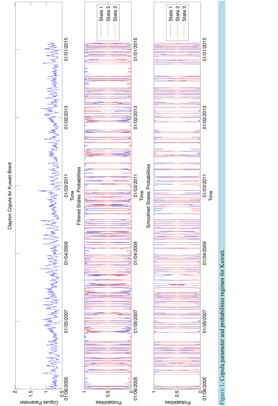
Figure 1.Copula parameter and probabilities regimes for Kuwait.
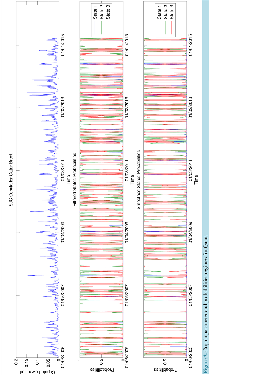
Figure 2.Copula parameter and probabilities regimes for Qatar.
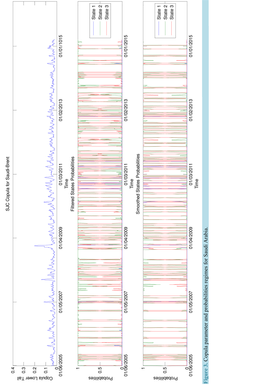
Figure 3.Copula parameter and probabilities regimes for Saudi Arabia.
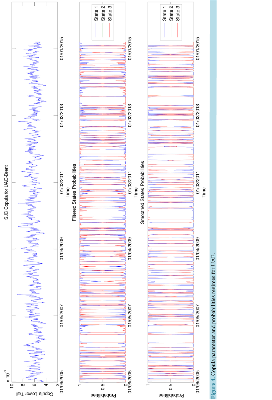
Figure 4.Copula parameter and probabilities regimes for UAE.
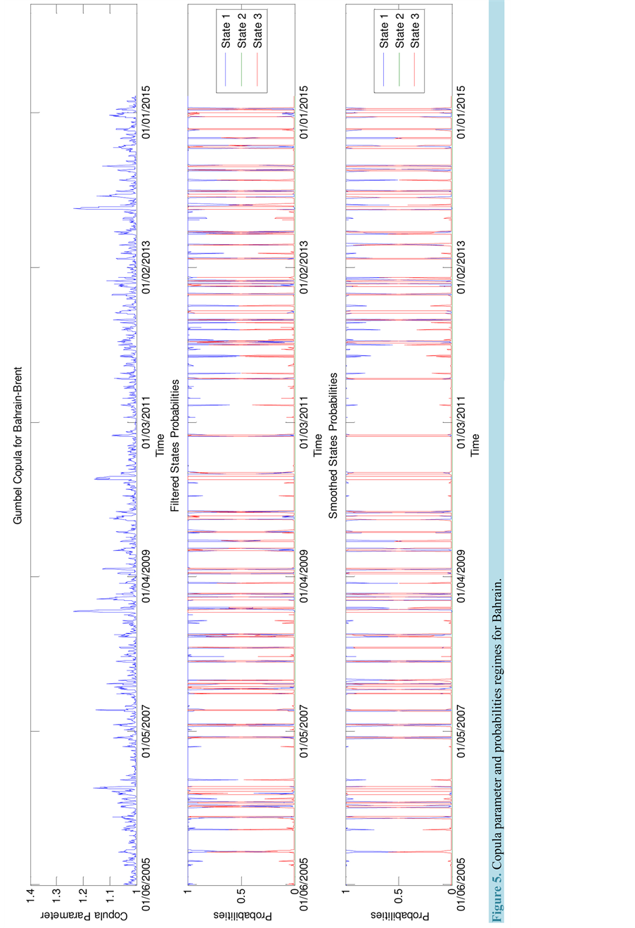
Figure 5.Copula parameter and probabilities regimes for Bahrain.
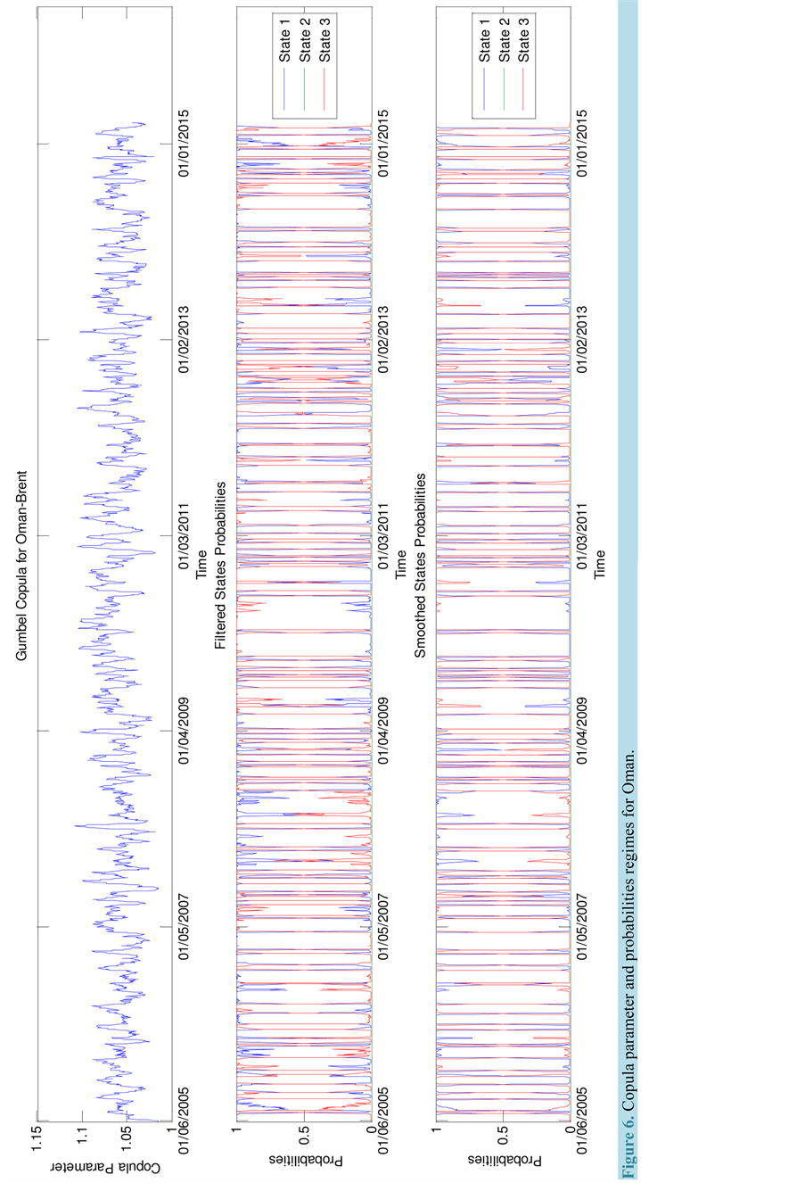
Figure 6.Copula parameter and probabilities regimes for Oman.
price changes and stock market returns. For Qatar, Saudi Arabia and the UAE (Figures 2-4), we can see a considerable change of dependence as the copula parameter varies over time. In regime 1 (pre-crisis regime), the tail dependence is relatively low, indicating no tail dependence. In regime 2 (crisis regime), the lower tail dependence drops significantly and positively with a biggest drop for Saudi Arabia. This could be attributed to the fact that Saudi Arabia is the largest oil producer and exporter. In regime 3, the lower tail dependence seems to be to the one found in the first regime. A similar behavior is observed in Kuwait (Figure 1), where the Clayton copula parameter is near 0 in regimes 1 and 3, reflecting independence. In regime 2, the Clayton copula parameter is positive, implying a strong positive dependence. For Bahrain and Oman (Figure 5 and Figure 6), the Gumbel copula parameter is close to 1 in regimes 1 and 3, thus indicating no dependence. In regime 2, the Gumbel copula parameter is greater than 1, implying a strong positive dependence.
These findings suggest some important implications. First, there is a higher dependence structure between oil price changes and all GCC stock market returns during the financial crisis period than during the calm ones (pre-crisis or post-crisis). This result means that the dependence structure between oil price changes and stock market returns is more intensified and suggests the presence of a contagion effect in sense of [52] and implies that diversification will be less effective and that holding a portfolio with oil assets and the stock market index during a financial crisis is subject to systematic risk. This result is in line with that of [3] , who reports that the sensitivity of GCC stock markets to oil price changes has jumped following the financial crisis period. It is similar to [25] , who find that the dependence between GCC stock market returns and oil price changes is regime-dependent. It is also consistent with that obtained by [21] [23] [24] [26] [27] , who find that the dependence structure between oil price changes and stock market returns has been strengthened following the financial crisis. As advanced by [24] , this result may be explained by the sharp decline in energy demand, caused by the economic downturn, which heavily affects the stock markets or by the rapid development of financial markets, that increases the exposure of oil prices to financial turmoil.
Second, during the financial crisis period, there is evidence of lower tail dependence in OPEC countries whereas in the non-OPEC countries, there is rather evidence of upper tail dependence. These findings have important implications for both investors who are interested in GCC stock markets, and for policymakers. During pre- and post-crisis periods, they can invest in all GCC stock markets to benefit from diversification and to reduce exposure to risk because the series are independent. During the financial crisis period, the investors who include oil as an asset in a diversified portfolio or energy risk managers who consider VaR (or other downside energy risk measures) should be particularly concerned about downside risk exposure and should emphasize the left side of the portfolio return distribution. Indeed, the risk diversification is less effective due to their stronger dependence and the investor must pay attention and the choice of the portfolio is related to whether the oil price is expected to increase or decrease. More precisely, if the oil price is expected to increase, a portfolio of OPEC stock market indices and oil can be better in terms of diversification because the series are not expected to boom together. In contrast, if the oil price is expected to decrease, a portfolio of non-OPEC stock market indices and oil can be preferred because the series are not expected to crash together.
4. Conclusions
This paper examines the presence of regime change in the dynamic dependence structure between oil price changes and stock market returns in six GCC countries during the period May 25, 2005 to March 31, 2015. In particular, we assume that there are three regime changes corresponding to low, high and crash volatility. The transition from one regime to other is conducted.
The econometric approach adopted is based on two steps. In a first step, we model the marginal distributions using an ARFIMA-FIAPARCH model with skewed-t distribution. We find evidence of dual long-range de- pendence and asymmetric reactions of the conditional variance to positive and negative shocks. In a second step, we focus on the dependence structure between filtered returns series using different Markov-switching time-varying copula functions.
For all countries, we find evidence of three-state Markov-switching regimes corresponding to pre-crisis, financial crisis and post-crisis regimes. More precisely, we see that in pre- and post-crisis regimes, there is no de- pendence. In contrast, in the financial crisis regime, there is a significant tail dependence. In particular, in OPEC countries (Qatar, Saudi Arabia, the UAE and Kuwait), we find lower tail dependence. In non-OPEC countries (Bahrain and Oman), we see upper tail dependence. The dependence structure seems to be related to oil production and consumption as well as to the importance of oil to its national economy. In particular, we find that Saudi Arabia, which is the largest oil producer and exporter and which presents the biggest market capitalization, shows the highest increase in lower tail dependence during the financial crisis period. Simulation results of VaR show that the proposed model outperforms the traditional time-varying copula model. Fur- thermore, these empirical findings are of great interest for investors in order to build profitable investment strategies. The fact that GCC stock market returns have different dependence structures to oil price changes implies valuable risk diversification opportunities across countries.
Cite this paper
Heni Boubaker,Nadia Sghaier, (2016) Markov-Switching Time-Varying Copula Modeling of Dependence Structure between Oil and GCC Stock Markets. Open Journal of Statistics,06,565-589. doi: 10.4236/ojs.2016.64048
References
- 1. Abou Zarour, B.A. (2006) Wild Oil Prices, but Brave Stock Markets! The Case of GCC Stock Markets. Operational Research, 6, 145-162.
http://dx.doi.org/10.1007/BF02941229 - 2. Basher, S.A. and Sadorsky, P. (2006) Oil Price Risk and Emerging Stock Markets. Global Finance Journal, 17, 224-251.
http://dx.doi.org/10.1016/j.gfj.2006.04.001 - 3. Arouri, M.E.H., Lahiani, A. and Nguyen, D.K. (2011) Return and Volatility Transmission between World Oil Prices and Stock Markets of the GCC Countries. Economic Modelling, 28, 1815-1825.
http://dx.doi.org/10.1016/j.econmod.2011.03.012 - 4. Jouini, J. (2013) Return and Volatility Interaction between Oil Prices and Stock Markets in Saudi Arabia. Journal of Policy Modeling, 35, 1124-1144.
http://dx.doi.org/10.1016/j.jpolmod.2013.08.003 - 5. Wang, Y., Wu, C. and Yang, L. (2013) Oil Price Shocks and Stock Market Activities: Evidence from Oil-Importing and Oil-Exporting Countries. Journal of Comparative Economics, 41, 1220-1239.
http://dx.doi.org/10.1016/j.jce.2012.12.004 - 6. Hammoudeh, S. and Aleisa, E. (2004) Dynamic Relationship among GCC Stock Markets and NYMEX Oil Futures. Contemporary Economic Policy, 22, 250-269.
http://dx.doi.org/10.1093/cep/byh018 - 7. Hammoudeh, S. and Choi, K. (2006) Behavior of GCC Stock Markets and Impacts of US Oil and Financial Markets. Research in International Business and Finance, 20, 22-44.
http://dx.doi.org/10.1016/j.ribaf.2005.05.008 - 8. Arouri, M.E.H. and Rault, C. (2010) Oil Prices and Stock Markets: What Drives What in the Gulf Corporation Council countries. Economie Internationale, 56, 41-56.
- 9. Arouri, M.E.H., Dinh, T.H. and Nguyen, D.K. (2010) Time-Varying Predictability in Crude Oil Markets: The Case of GCC Countries. Energy Policy, 38, 4371-4380.
http://dx.doi.org/10.1016/j.enpol.2010.03.065 - 10. Aloui, C. and Jammazi, R. (2009) The Effects of Crude Oil Shocks on Stock Market Shifts Behaviour: A Regime Switching Approach. Energy Economics, 31, 789-799.
http://dx.doi.org/10.1016/j.eneco.2009.03.009 - 11. Maghyereh, A. and Al-Kandari, A. (2007) Oil Prices and Stock Markets in GCC Countries: New Evidence from Nonlinear Cointegration Analysis. Managerial Finance, 33, 449-460.
http://dx.doi.org/10.1108/03074350710753735 - 12. Arouri, M.E.H. and Fouquau, J. (2009) On the Short-Term Influence of Oil Price Changes on Stock Markets in GCC Countries: Linear and Nonlinear Analyses. Economics Bulletin, 29, 806-815.
- 13. Jouini, J. (2013) Stock Markets in GCC Countries and Global Factors: A Further Investigation. Economic Modelling, 31, 80-86.
http://dx.doi.org/10.1016/j.econmod.2012.11.039 - 14. Balcilar, M., Demirer, R. and Hammoudeh, S. (2013) Investor Herds and Regime-Switching: Evidence from Gulf Arab Stock Markets. Journal of International Financial Markets Institutions and Money, 23, 295-321.
http://dx.doi.org/10.1016/j.intfin.2012.09.007 - 15. Hamilton, J.D. (2003) What Is an Oil Shock. Journal of Econometrics, 113, 363-396.
http://dx.doi.org/10.1016/S0304-4076(02)00207-5 - 16. Zhang, D. (2008) Oil Shock and Economic Growth in Japan: A Nonlinear Approach. Energy Economics, 30, 2374-2390.
http://dx.doi.org/10.1016/j.eneco.2008.01.006 - 17. Cologni, A. and Manera, M. (2009) The Asymmetric Effects of Oil Shocks on Output Growth: A Markov-Switching Analysis for the G-7 Countries. Economic Modelling, 26, 1-29.
http://dx.doi.org/10.1016/j.econmod.2008.05.006 - 18. Mohanty, S.K., Nandha, M., Turkistani, A.Q. and Alaitani, M.Y. (2011) Oil Price Movements and Stock Market Returns: Evidence from Gulf Cooperation Council (GCC) Countries. Global Finance Journal, 22, 42-55.
http://dx.doi.org/10.1016/j.gfj.2011.05.004 - 19. Awartani, B. and Maghyereh, A.I. (2013) Dynamic Spillovers between Oil and Stock Markets in the Gulf Cooperation Council Countries. Energy Economics, 36, 28-42.
http://dx.doi.org/10.1016/j.eneco.2012.11.024 - 20. Nguyen, C.C. and Bhatti, M.I. (2012) Copula Model Dependency between Oil Prices and Stock Markets: Evidence from China and Vietnam. Journal of International Financial Markets, Institutions and Money, 22, 758-773.
http://dx.doi.org/10.1016/j.intfin.2012.03.004 - 21. Aloui, R., Hammoudeh, S. and Nguyen, D.K. (2013) A Time-Varying Copula to Oil and Stock Market Dependence: The Case of Transition Economies. Energy Economics, 39, 208-221.
http://dx.doi.org/10.1016/j.eneco.2013.04.012 - 22. Patton, A.J. (2006) Modelling Asymmetric Exchange Rate Dependence. International Economic Review, 47, 527-556.
http://dx.doi.org/10.1111/j.1468-2354.2006.00387.x - 23. Wen, X., Wei, Y. and Huang, D. (2012) Measuring Contagion between Energy Market and Stock Market during Financial Crisis: A Copula Approach. Energy Economics, 34, 1435-1446.
http://dx.doi.org/10.1016/j.eneco.2012.06.021 - 24. Zhu, H.-M., Li, R. and Li, S. (2013) Modelling Dynamic Dependence between Crude Oil Prices and Asia-Pacific Stock Market Returns. International Review of Economics and Finance, 29, 208-223.
http://dx.doi.org/10.1016/j.iref.2013.05.015 - 25. Naifar, N. and Al Dohaiman, M.S. (2013) Nonlinear Analysis among Crude Oil Prices, Stock Markets Return and Macroeconomic Variables. International Review of Economics and Finance, 27, 416-431.
http://dx.doi.org/10.1016/j.iref.2013.01.001 - 26. Boubaker, H. and Sghaier, N. (2014) Instability and Dependence Structure between Oil Prices and GCC Stock Markets. Energy Studies Review, 20, 50-65.
http://dx.doi.org/10.15173/esr.v20i3.555 - 27. Boubaker, H. and Sghaier, N. (2014) Measuring the Contagion Effect between Energy and Stock Markets in Ten MENA Countries Using Copulas with Local Change Points. Working Paper, IPAG Business School.
- 28. Hamilton, J.D. (1994) Time Series Analysis. Princeton University Press, Princeton.
- 29. Rodriguez, J.C. (2007) Measuring Financial Contagion: A Copula Approach. Journal of Empirical Finance, 14, 401-423.
http://dx.doi.org/10.1016/j.jempfin.2006.07.002 - 30. Garcia, R. and Tsafack, G. (2011) Dependence Structure and Extreme Comovements in International Equity and Bond Markets. Journal of Banking and Finance, 35, 1954-1970.
http://dx.doi.org/10.1016/j.jbankfin.2011.01.003 - 31. Cholette, L., Heinen, A. and Valdesogo, A. (2009) Modeling International Financial Returns with a Multivariate Regime-Switching Copula. Journal of Financial Econometrics, 7, 437-480.
http://dx.doi.org/10.1093/jjfinec/nbp014 - 32. Wang, Y.-C., Wu, J.-L. and Lai, Y.-H. (2013) A Revisit to the Dependence Structure between the Stock and Foreign Exchange Markets: A Dependence-Switching Copula Approach. Journal of Banking and Finance, 37, 1706-1719.
http://dx.doi.org/10.1016/j.jbankfin.2013.01.001 - 33. Da Silva Filho, O.C., Ziegelmann, F.A. and Dueker, M.J. (2012) Modeling Dependence Dynamics through Copulas with Regime Switching. Insurance: Mathematics and Economics, 50, 346-356.
http://dx.doi.org/10.1016/j.insmatheco.2012.01.001 - 34. Sklar, A. (1959) Fonctions de Répartition à n Dimensions et Leurs Marges. Publications de l’Institut Statistique de l’Université de Paris, 8, 229-231.
- 35. Joe, H. (1997) Multivariate Models and Dependence Concepts. Monographs in Statistics and Probability. Chapman and Hall, London.
http://dx.doi.org/10.1201/b13150 - 36. Nelson, R. (2006) An Introduction to Copulas. Springer-Verlag, New York.
- 37. Patton, A.J. (2012) A Review of Copula Models for Economic Times Series. Journal of Multivariate Analysis, 110, 4-18.
http://dx.doi.org/10.1016/j.jmva.2012.02.021 - 38. Gumbel, E.J. (1960) Distributions de valeurs extrêmes en plusieurs dimensions. Publications de l’Institut de Statistique de l’Université de Paris, 9, 171-173.
- 39. Clayton, D.G. (1978) A Model for Association in Bivariate Life Tables and Its Applications in Epidemiological Studies of Familial Tendency in Chronic Disease Incidence. Biometrika, 65, 141-151.
http://dx.doi.org/10.1093/biomet/65.1.141 - 40. Joe, H. and Xu, J. (1996) The Estimation Method of Inference Functions for Margins for Multivariate Models. Technical Report No. 166, Department of Statistics, University of British Columbia, Vancouver.
- 41. Genest, C., Ghoudi, K. and Rivest, L.-P. (1995) A Semiparametric Estimation Procedure of Dependence Parameters in Multivariate Families of Distributions. Biometrika, 82, 543-552.
http://dx.doi.org/10.1093/biomet/82.3.543 - 42. Reboredo, J.C. (2011) How Do Crude Oil Prices Co-Move? A Copula Approach. Energy Economics, 33, 948-955.
http://dx.doi.org/10.1016/j.eneco.2011.04.006 - 43. Baillie, R.T., Bollerslev, T. and Mikkelsen, H.O. (1996) Fractionally Integrated Generalized Autoregressive Conditional Heteroskedasticity. Journal of Econometrics, 74, 3-30.
http://dx.doi.org/10.1016/S0304-4076(95)01749-6 - 44. Bollerslev, T. (1986) Generalized Autoregressive Conditional Heteroskedasticity. Journal of Econometrics, 31, 307-327.
http://dx.doi.org/10.1016/0304-4076(86)90063-1 - 45. Engle, R.F. and Bollerslev, T. (1986) Modelling the Persistence of Conditional Variance. Econometric Reviews, 5, 1-50.
http://dx.doi.org/10.1080/07474938608800095 - 46. Glosten, L.R., Jagannathan, R. and Runkle, D. (1993) On the Relation between the Expected Value and the Volatility of the Nominal Excess Return on Stocks. Journal of Finance, 48, 1779-1801.
http://dx.doi.org/10.1111/j.1540-6261.1993.tb05128.x - 47. Tse, Y.K. (1998) The Conditional Heteroscedasticity of the Yen-Dollar Exchange Rate. Journal of Applied Econometrics, 13, 49-55.
http://dx.doi.org/10.1002/(SICI)1099-1255(199801/02)13:1<49::AID-JAE459>3.0.CO;2-O - 48. Hansen, B. (1994) Autoregressive Conditional Density Estimation. International Economic Review, 35, 705-730.
http://dx.doi.org/10.2307/2527081 - 49. Fernández, C. and Steel, M. (1998) On Bayesian Modelling of Fat Tails and Skewness. Journal of the American Statistical Association, 93, 359-371.
- 50. Garcia, R. (1998) Asymptotic Null Distribution of the Likelihood Ratio Test in Markov Switching Models. International Economic Review, 39, 763-788.
http://dx.doi.org/10.2307/2527399 - 51. Ang, A. and Bekaert, G. (2002) Regime Switches in Interest Rates. Journal of Business and Economic Statistics, 20, 163-182.
http://dx.doi.org/10.1198/073500102317351930 - 52. Forbes, K.J. and Rigobon, R. (2002) No Contagion, Only Interdependence: Measuring Stock Market Comovements. Journal of Finance, 57, 2223-2261.
http://dx.doi.org/10.1111/0022-1082.00494
NOTES

*Corresponding author.

1The GCC countries include six countries, namely, Bahrain, Kuwait, Oman, Qatar, Saudi Arabia and United Arab Emirates (UAE).
2The dummy variable takes the value of 1 if the oil price changes are positive and 0 otherwise.

3For an introduction to copulas, see [35] and [36] and for a recent review, see [37] .

4There are many mays of capturing possible time variation in the dependence structure. In this paper, we assume following [22] that the functional form of the copula remains fixed over the sample while the parameters vary according to some evolution equation.
5This choice is justified by the empirical results obtained in Section 3.3.

6The choice of the dual long-memory model is proved by the empirical results obtained for the returns series considered.

7For providing asymptotic theory for the estimator, see [33] .

8To check the stationarity, we apply the unit root tests without and with structural breaks. We find evidence of stationarity. These results are not reported here but are available upon request.

9We do not report autocorrelation functions and spectral densities. These are available on request.
10p and q are determined according to information criteria.

11Note that  at the 1% level.
12In this paper, we do not report the results of statistic LR test. These are available on request.

13Here, we do not report the empirical results, these are supplied upon request.
14We note that the selected copula in terms of LL is one with lowest LL, since in our estimation we minimize (-LL) rather than maximize (LL).
15Here we consider a portfolios composed of two assets.

16Recall that the Clayton copula is characterized by lower tail dependence. For SJC copula  are higher than
  indicating also lower tail dependence.
17Note that the Gumbel copula is characterized by upper tail dependence.