Open Journal of Statistics
Vol.05 No.03(2015), Article ID:55993,17 pages
10.4236/ojs.2015.53021
Trace of the Wishart Matrix and Applications
T. Pham-Gia1*, Dinh N. Thanh2, Duong T. Phong3
1Université de Moncton, Moncton, Canada
2University of Science, Hochiminh City, Vietnam
3Ton Duc Thang University, Hochiminh City, Vietnam
Email: *thu.pham-gia@umoncton.ca, dnthanh@hcmus.edu.vn, dtphong@itam.tdt.edu.vn
Copyright © 2015 by authors and Scientific Research Publishing Inc.
This work is licensed under the Creative Commons Attribution International License (CC BY).
http://creativecommons.org/licenses/by/4.0/


Received 19 January 2015; accepted 22 April 2015; published 27 April 2015
ABSTRACT
The trace of a Wishart matrix, either central or non-central, has important roles in various multivariate statistical questions. We review several expressions of its distribution given in the literature, establish some new results and provide a discussion on computing methods on the distribution of the ratio: the largest eigenvalue to trace.
Keywords:
Trace, Wishart Matrix, Sphericity, Latent Roots, A-Hypergeometric Functions, Humbert Function

1. Introduction
Let  be a normal vector and
  be a sample taken from this multivariate normal
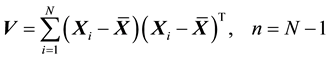
population. Classical results show that the sample mean vector  is independent of the sample
covariance matrix , where
 ,
,
and they are distributed respectively, as a normal vector  and a central Wishart matrix
 , with
  degrees of freedom and covariance matrix
 , with density
 , (1)
, (1)
where ,
,  means that
  is positive definite matrix, and
 ,
,
 .
.
If , the distribution is singular and no density exists. The case of pseudo-Wishart matrices will not be considered in detail here.
Several important results in Multivariate analysis are associated with either the determinant, trace or the eigenvalues of this matrix.
For , we have the non-central Wishart
 , with non-centrality parameter
 , which has the more complicated density expression:
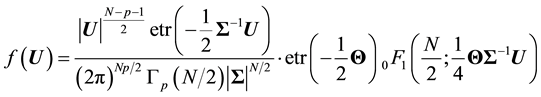 , (2)
, (2)
where , and
, and  is the hypergeometric function with one matrix argument, and reduces to (1) when
 .
.
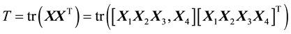
We can also have the matrix  formed by the n column vectors
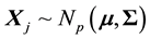 , and consider the product matrix
 . We have then
 , where
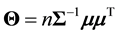 . More general is the case where
  are independent observations from
 ,
,  , with different values for
 . We then form the
  matrix
  and we again have:
 , where.
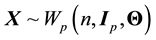
If we consider at the start the  rectangular matrix as variate, i.e.
 ,
,  , the product matrix
  is Wishart, i.e.
 , where
 , central if
  and
and , or non-central with density (2) otherwise.
We wish to avoid too technical results in this article, that could digress us from the real purpose of this survey- type article, which is to gather results on the distribution of the trace of the Wishart matrix, that are still scattered in the literature. But several new research results related to this trace, are also presented. In most cases, we will present both the central and the non-central cases, or the null and non-null distributions of a test criterion. It is also natural that we will encounter zonal polynomials, the values of which are not completely known. Finally, due to the extremely complicated mathematical expressions of certain results we will refer the reader to the original publications when this approach appears to be more convenient.
The non-central Wishart distribution has an important role in theoretical Multivariate analysis, but recently has also found some applications, for example in Image Processing [1] .
The Wishart distribution has been generalized in several directions and the most general extension of the Wishart is made by Díaz-García and Guttiérez-Jáimez [2] to which we refer the reader for additional details. Concerning the product of several positive common random univariate random variables, or the ratio of two positive random variates, H-function, or G-function distributions [3] will be used but we will not discuss the best technique to compute the values of these functions by the residue theorem, since this challenging mathematical problem is already an important topic in itself. Maple and Mathematica can deal with fairly complex cases.
In Section 2 we will first recall several special functions that will be used later. In Section 3 we consider the central Wishart distribution and its trace. Similar results are established for the non-central Wishart and its trace in Section 4. Section 5 studies the moments of the trace while Section 6 considers the Wishartness of some quadratic forms. Section 7 considers the sphericity problem where the trace of the Wishart matrix has an important role. Finally, Section 8 considers the latent roots and their ratios to the trace and shows the need of further research in this area. It also proposes the simulation approach that has proven to be very effective in some of our previous works.
2. Some Special Functions
2.1. Special Functions
Table 1 gives all the probability densities treated here.
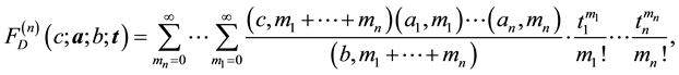
Advanced statistics make use of several special functions and integral transforms: the Humbert function of the second kind and the Lauricella D-function. They are both defined as infinite series, and extended by analytic continuation and are related to each other. We define:

Table 1. Table of densities.
1) The Lauricella D-function, in  parameters and
  scalar variables, by:
where
 ,
,
and , which converges for all values of
 ,
, .
.
2) Similarly, we define the Humbert function, in  parameters and
  scalar variables, by:
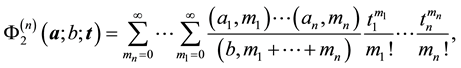
which converges for all values of .
.
We have the Dirichlet distribution (in n + 1 parameters and n variables), 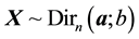 , with
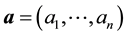 , which also has a key role in multivariate analysis. It has density:
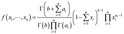 ,
,
where ,
, .
.
The  function in
  variables is, in fact, the Laplace transform of the Dirichlet distribution. We have:
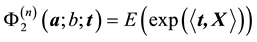 ,
,
where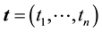 ,
, 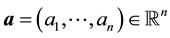 and
and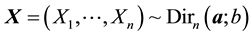 .
.
The relation between  and
and  is [4] :
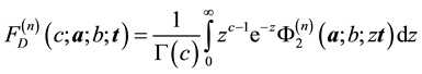 . (3)
. (3)
An extension of  to the matrix variates is given by [5] and an application of
  in renewal processes can be found in [6] . On the other hand,
 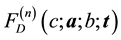 has several integral representations, the most interesting one should be Euler’s type representation, as an hypergeometric integral in one variable:
 , (4)
, (4)
also known as Picard’s integral for .
.
2.2. Integral Representations
Formulas (3) and (4) above allow us to use several interesting mathematical results related to Hypergeometric integrals, which are the focus of much recent work by Gelfand, Krapalov and Zelevinsky [7] , named GKZ integrals. They are also known under the topic of A-Hypergeometric functions [8] during the last thirty years. The various hypergeometric functions in several variables, defined differently according to how variables are summed, and named as Horn, Lauricella, Wright, MacRobert functions etc., can now be integrated into a single approach. The introduction of Grobner basis in their study, by Saito, Sturmfels and Takayama [9] , has lead to other important results.
Since some of the results obtained by our research group are highly mathematical we do not reproduce them here but they can be obtained by writing to the third author.
The trace of a square matrix is defined as the sum of its diagonal elements, and is sometimes used to measure the total variance. So, let , and its univariate density is under study in this article.
For the central Wishart distribution, we will show in the next two sections that when , the trace,
  , is a central Chi-square variable.
3. Central Wishart Distribution
3.1. Two Cases for 
Essentially there are two cases:
1) The matrix sigma is diagonal, : There are several ways to determine the distribution of
 :
:
Bartlett’s classical decomposition of the Wishart matrix, 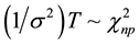 , is as follows: Let
  where
where  is upper-triangular
  matrix with positive diagonal elements. Then the elements,
  ,
,  , are all independent, with the diagonal elements
  being
being ,
,  , while the off-diagonal elements
  being
being
 .
.
Since we have , the diagonal elements will give a chi square with
  degree of freedom, while the off-diagonal give a chi square with
  degree of freedom. Adding them together we then have a chi square with
  degree of freedom, i.e.
 .
.
Another approach: Consists in considering the latent roots on the diagonal matrix  equivalent to
 ,
,  , with
  is orthogonal matrix. These latent roots are
 ,
,  being in-
dependent, with  being a chi square with
  degree of freedom.
REMARK: In the more general case when , then
 . The trace is then a
linear combination of independent central Chi-squares, each with  degree of freedom.
PROPOSITION 1. Let ,
,  be the traces of
  independent Wishart matrices
 .
.
Then we have , with
 . Furthermore, the product
  and ratios
 ,
,  ,
,  ,
,
can have their densities expressed as G-functions.
PROOF: Immediate from the above results and from [10] , where products and ratios of G-functions are presented.
QED.
2) The matrix sigma is not diagonal, :
:
Results are quite complicated for this case since it involves zonal polynomials, whose expressions are only known for simple cases ([11] , p. 341).
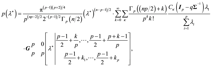
For , the density is a mixture of gamma distributions, and various expressions of it are available in the statistical literature.
For ,
,  has density
 ,
,
where ,
,  and
and  is the zonal polynomial.
We have the usual notations:  is arbitrary (chosen to be
 ), where
  and
and 
are respectively the largest and the smallest latent roots of matrix ,
, is a partition of
with ,
,  is the zonal polynomial corresponding to
 ,
,  and
and
 .
.
3.2. Other Expressions
Mathai and Pillai (1980) give another expression, quite similar:
 .
.
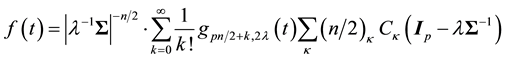
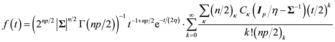
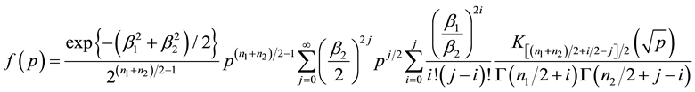
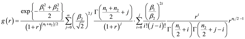
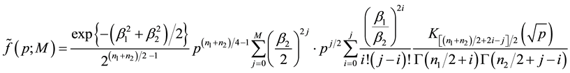
However, using Mellin Transform methods [12] gives the following density function for , which avoids the use of zonal polynomials
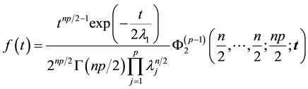 , (5)
, (5)
where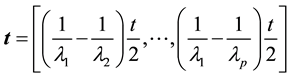 , and
, and  is the Humbert hypergeometric function of the second type mentioned earlier.
4. Non-Central Wishart Distribution
4.1. The Non-Central Chi-Square Distribution
This distribution is present in many aspects of statistics. Its density is given in our table of densities but below is an alternate expression.
Let  be the modified first Bessel function of the 1st kind
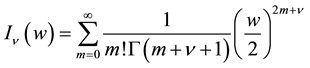 .
.
The associated Bessel density is:
 . (6)
. (6)
A particular case of (6) is the non-central Chi-square density with  degrees of freedom and non-centrality parameter
 ,
,  , obtained when
 .
.
Its density is then [13] :
 , (7)
, (7)
where .
.
Using the above functions Laha [14] proved that the reproductive property of the non-central Chi-square, i.e. the sum of  independent non-central Chi-square is itself a non-central Chi-square, with parameters
  and
and  being the corresponding sums of the related parameters.
The density of the product or quotient of two non-central chi square variables can be established in closed form using either Fourier transform [14] or Mellin Transform [13] . Following the latter we have:
PROPOSITION 2. Let ,
,  , be two independent non-central Chi-square random variables
 , with densities given by (7). Then the product
  has as density
 , (8)
, (8)
where  is the modified Bessel function of the third kind and given by
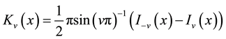 .
.
While the ratio  has as density
 . (9)
. (9)
4.2. The Non-Central Wishart Distribution
As given by (2), its trace  can now be shown to be a non-central Chi-square in some cases.
First, a simple case is the linear non-central case where the non-centrality parameter is concentrated at one component, can be treated as the central case [15] . For a normal vector , this will happen when only the first component of
  is different from 0 and for a normal
  matrix
 , when only the first line of
  is different from 0. More precisely, let
 ,
,
where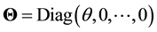 . Then there is a decomposition of
 , where
  is lower triangular with independent elements such that only the first element is a non-central Chi-square, i.e.
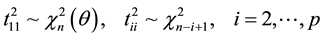 ,
,
and ,
, .
.
Hence we have
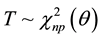 . (10)
The above result on Bessel function distributions now allows us to have the density of sums, product and ratios of the traces of independent linear non-central Wishart distributions. We have the following
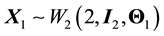
THEOREM 1. Let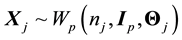 ,
,  with
with  and
and  and
and  be independent, and let
  and
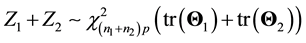
and  be the two respective traces. The sum
  is a non-central Chi-square, while for the product
  and ratio
 , their densities can be expressed in closed form, using (8) and (9).
PROOF. Applying (10), we have , and similarly for
 .
.
For , we have
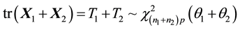 .
.
For the product, we have  having density given by (8) for its first component, while for the ratio
 , it has density (9) where
  and
and , also for its first component. We then use the reproductive property of the non-central Chi-square.
QED.
4.3. Numerical Example
We can use (8) and (9) to graph the density of the product and quotient of the two traces. Some computer algebra software, Maple and Mathematica, for example, can do the computation in (8) (9) as an infinite series. But the computation, especially for (8), is very slow. Here, we approximate (8) by taking a large number of terms.
 ,
,
with the value , this approximation seems to be very good. Let
 and,
and,
where 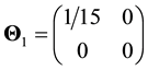 and
and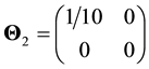 . We get the following graphs of densities of
 ,
,
 ,
,  and
and , where the horizontal scales are very different (Figure 1).
In the case of planar non-centrality, i.e. , as remarked by Anderson [16] , we run into an infinite series of Bessel functions and formulas become very complicated.
4.4. Case 
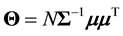
We have the following argument, based on the Moment Generating Function (MGF) of  given by [17] :
For ,
,  , we let
 ,
,  , and
, and  , we have
 .
.
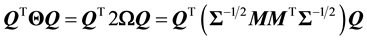
Here we set , as in [17] where it is shown that the MGF of
  is given by
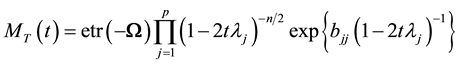 ,
,
where  is the j-th diagonal element of
 ,
,  is the orthogonal matrix such that
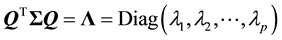 .
.
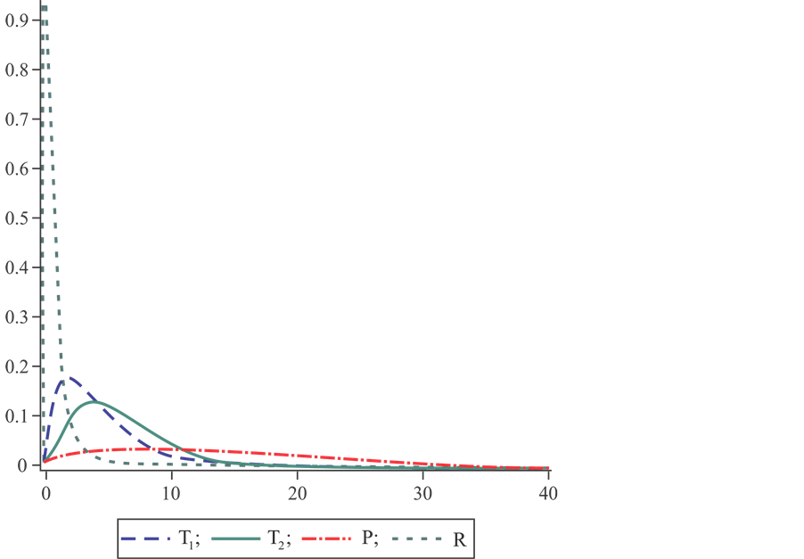
Figure 1. Density of ,
,  ,
,  and
and .
.
Using  and, writing
 , we have
 .
.
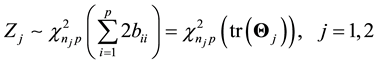
Using the MGF of the Non-Central Chi-square in our table of densities we have the expression of the trace  in terms of a linear combination of non-central Chi square variables with
  degrees of freedom each and non- centrality parameter
 , the j-th diagonalelement of
 , i.e.
 , (11)
where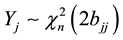 , with
  independent.
The density of  can be given under a variety of forms by inverting the MGF of
 . [12] , for example, gives 3 forms (see Section 4.7).
The density of a linear combination of non-central chi-square variables has been the subject of investigation by several authors, since it is associated with quadratic forms in normal variables. Ruben [18] , Press [19] and Hartville [20] seemed to be among the first investigators. More recent is the work of Provost and Ruduik [21] .
The approach using Laguerre expansions seems promising, as shown by some authors, including Castano- Martinez and Lopez-Blasquez [22] . But all the formulas obtained are quite complicated and we refer the readers to these articles. It should be mentioned that using the same MGF, Kourouklis and Moschopoulos [23] give this density as an infinite combination of gamma densities.
4.5. A Simulation Study
Simulation for the density of the trace of non-central Wishart matrix. Following 4.4, let the covariance matrix be
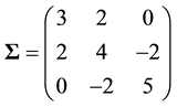 , positive, definite. And the four means be:
 .
.
With the above means and covariance matrix, we have:
 , ,
, ,
 , ,
, ,
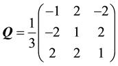
and the matrix  is computed using:
 .
.
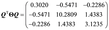 .
.
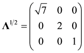
We finally have: ,
,  ,
,  and
and ,
,  ,
, .
.
Now, two approaches are used to obtain the density of :
:
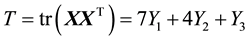
1) Direct approach 1: We use
 .
.
We use Matlab command  to generate 4 normal vectors
 ,
,  , from which we obtain a value of the trace
 . Doing this operation 10,000 times we have the density of
  given by Figure 2.
2) Approach using non-central Chi-squares: We use
 ,
,
where ,
,  , and
, and .
.
We use Matlab routine  to generate observations
  from
from , and compute
 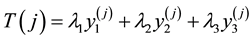 10000 times and we have Figure 3.
We can see that the two graphs are very close to each other.
4.6. Modified Traces
The influence of  on
on  is through the coefficients
 . If we remove these coefficients we have the modi-
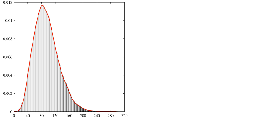
Figure 2.  using Matlab. mndvn.
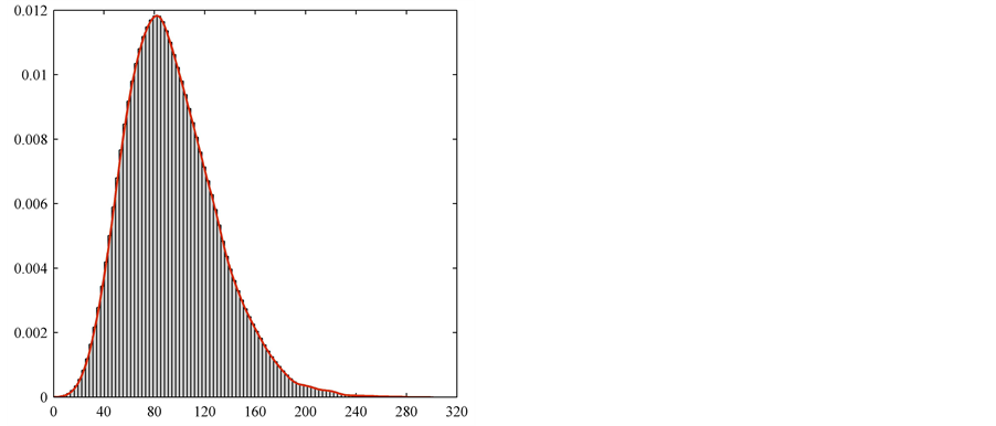
Figure 3.  using Matlab.ncxrdn.
fied trace .
.
PROPOSITION 3: Let ,
,  with non-diagonal
 , be independent and
 ,
,  be their traces. Let Zi,
  be the “modified traces” obtained from Ti by taking
 . Then the sum
 , and of the product,
  and ratio
 , can be obtained in closed form.
PROOF: Using (11) with  and
and
 .
.
Thus, we have
 ,
,
and their sum  is itself a non-central Chi- square, with, as parameters the corresponding sums of individual parameters, i.e.
 .
.
For the product: , we have the same distribution as the product of two non-central Chi-squared random variables, i.e. its density is given by (8). Similarly for the ratio, using (9).
QED.
Glueck and Muller [24] also relate the trace of any type of Wishart, singular or nonsingular, central or non- central, true or pseudo, to a weighted sum of non-central Chi-squared random variables and constants. However, the expression of this density is not given, although computational methods are presented, either approximate or permitting to prescribe a degree of accuracy.
4.7. Some Expressions of the Density of 
For some values of the parameters, there can be closed form expression for the density of . For example, [12] gives this density when
  is even (or the sample size
  is odd). The formula is however complicated, with reference to other works.
When the general case we have an expression similar to (5), but preceded by the non-central factor:
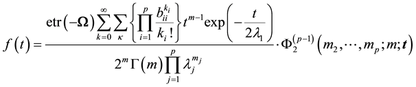 , (12)
with ,
, , and
, and ,
, .
.
where ,
, ,
,  ,
,  ,
, .
.
In terms of zonal polynomials, we have Formula (14) of [12] using common zonal polynomials, or a more compact formula, using Davis expended zonal polynomials .
.
 . (13)
For  and
and ,
, .
.
5. Moments of the Trace
The trace of  is present in the expressions of several of its moments, and moments are frequently easier to
obtain than densities themselves. For example, the r-th cumulant of ,
,  , which is the coefficient of
  in
in
the expansion of , where
  is the moment generating function of
  is found in [17] to be
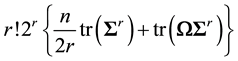 , which gives the mean of the trace
 , a result
also found in [25] . Saw [26] , and Shah and Khatri [27] proved several other results on moments of the trace of the non-central Wishart.
Some results are unexpected. For example, for , and
, and  is a
is a  constant matrix:
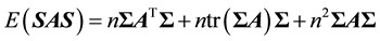 , and using zonal polynomials,
 ([15] , p. 98 and p. 106).
Several other equalities can be found in the same reference.
Letac and Massam [28] , on the other hand, computed the moments of the Wishart matrix , of the form
 , where
  is an invariant polynomial in the entries of the matrix
 , i.e. depending only on the eigenvalues of
 . Finally, there are several results available in the literature on the expectation of
 , which is the sum of all principal minors of order j of matrix
 . For example, for
 , we have:
 and,
and,
where .
.
6. The Wishartness of Certain Quadratic Forms
For , it is of interest to look for more general quadratic forms that could also be Wishart.
There are 3 cases of Quadratic forms:
・  is a unidimensional random variable when
 . We are interested at
  being a non-central Chi-square variable.
・  is a matrix if
 , where
 . We are interested in the condition for this matrix to be Wishart.
・ Similarly,  is a random matrix, possibly Wishart when
  is a
is a  normal random matrix.
PROPOSITION 4. ([15] , p. 256-257) Let , where
 . Then the necessary
and sufficient condition for  to be distributed as
  is that
  is idempotent of rank
 . A similar condition applies to
  to be
to be .
.
The trace  of
of  in these cases can be studied as previously. We will not elaborate on this point.
7. Sphericity Testing Criterion
In this section we limit ourselves to the vector case, i.e. of . Understandably, as seen from what precedes, the case
  is important, and this test would permit us to accept, or not, that the matrix is diagonal with same diagonal value.
7.1. Sphericity Test
An interesting property of the Gamma distribution in shape parameter  and scale parameter
 ,
,  , is that, for a random sample of observations the distribution of the arithmetic mean to the geometric mean is independent of the parameters [29] . An application in telecommunication is given by [30] .
Let  and let
  be a sample from this distribution. Let
 .
.
In testing the hypothesis 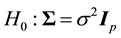 (or the
  components are equally variable), called sphericity, we can use:
1) The classical likelihood ratio criterion (LRC),  , first used by Mauchly [31]
 . (14)
The LRC above is hence the ratio of the geometric mean of the eigenvalues to their arithmetic mean. The null-distribution is the distribution of this criterion under  is the density of the product of betas of the first kind,
 , (15)
where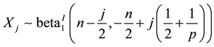 ,
,
as shown by [32] . This product can be shown to have a G-function density, namely
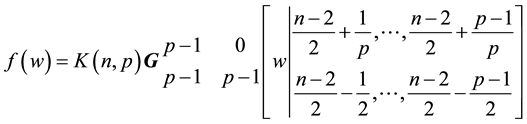 , (16)
where , and
, and
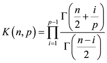 .
.
2) The product of 2 independent beta products [16] :
 ,
,
with 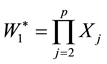 and
and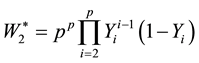 , where
 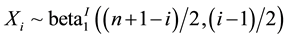 are mutually independent from each other, while
 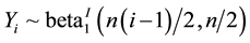 are also mutually independent.
・  is the test criterion for
 : The matrix is diagonal, and
・  is the criterion for
 : The diagonal elements are equal.
Their product is
 .
.
Since these two tests are in fact independent the product of the two criteria gives the above sphericity test criterion. [32] has adopted a simulation approach to deal with this product.
7.2. Bartlett’s Test
In univariate statistics, using  different samples to test that the variances of
  independent normal popula-
tions are equal, we have Bartlett’s test for homogeneity, based on , where
 ,
,
with .
.
When the samples have the same size, Glaser [33] has shown that the null distribution of  is a product
of independent betas: , where
 ,
,
n is sample size and  is shape parameter of the Gamma distribution.
  is the ratio of the geometric mean to the arithmetic mean.
But when these sizes are different [33] shows that the distribution of Bartlett’s statistic, which now is the adjusted ratio of weighted geometric mean of the sample variances to their weighted arithmetic mean, can be obtained with incomplete beta functions.
Gleser ([34] ) considered the two criteria  and
and  above and discussed the interesting relationship between Bartlett’s test and the sphericity test, which become equivalent under a change of variables. In the case of non-normality, Hartley’s test or Levene’s test, can be used to the same purpose.
Accepting the hypothesis of sphericity allows us to proceed on to other topics, such as analysis of variance using repeated measures. A generalization of this test to  covariance matrices is possible, and is often known as the Mendoza test.
7.3. Non-Null Distribution
When , we have the non-null distribution of
 .
.
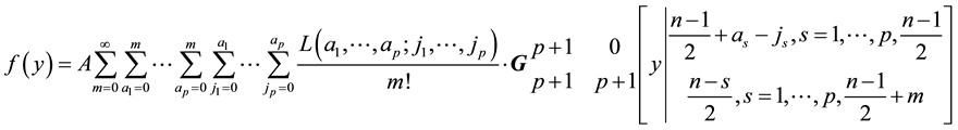
1) Khatri and Srivastava [35] gives the following expression for the density of the LRC, using both zonal polynomials and Meijer functions:
where  is the zonal polynomial associated with
 .
.
2) [36] propose a convenient strictly numerical method to approximate the power and test size under non- sphericity.
REMARKS. The non-null density in testing diagonality, as given in [37] , is a multiple infinite series involving Meijer functions:
 ,
,
where ,
,  is defined in [37] .
Again, here, the computation of the values of this expression is very complicated and we refer the reader to the original paper.
8. Distribution of Ratios of Latent Roots to the Trace
This distribution has attracted renewed interest lately due to its uses in Physics, on random matrices. Krishnaiah and Shurmann [38] were among the first authors to investigate the distributions of these ratios.
The Simulation approach: These distributions have been mentioned by [39] and Johnstone [40] in the context of random matrices. There, the limit theorems are those of Tracy-Widom, or TW, and Wigner. In particular, Nadler reports that, under the hypothesis that , with
 , than an approximate explicit expression of the distribution of this ratio
 , where
  is the largest latent root, can be derived, taking into consideration the second derivative of the TW distribution. Computation and simulation methods are used to derive numerical results.
1) Central case:
a) When the matrix sigma is diagonal:
Let  be the latent roots of the sample covariance matrix
 . The ratio of two latent roots
  is also called “condition number” in regression and is associated with collinearity. Troskie [41] gives a very complicated formula based on change of variable technique for the densities of these ratios, which we do not reproduce here. For the ratio of the largest to the trace
 , this density is not even tractable. However, [42] gives a relation between the exact null-distribution of the j-th largest root and the distribution of the ratio of this root to the trace, but only for
 .
.
b) When the matrix sigma is not diagonal:
This is even more complex and no result is available on this case. The only resort is by simulation, as in Pham-Gia and Turkkan (2010). Simulation of random matrices, using the appropriate technique, can be very accurate, as shown by several articles by Pham-Gia and Turkkan [39] [43] .
2) Non-central case:
This case is naturally more complicated than the previous one and the simulation approach seems to be the only recourse.
Example
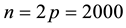
We give below the simulation results related to the ratio . Where
  are latent roots of matrix
  with 10,000 generated observations in cases:
1) ,
,  ,
, .
.
2) ,
,  , and
, and , where
 ,
, .
.
The simulation results are given by Figure 4 & Figure 5.
9. Conclusions
We have gathered here several important research results related to the trace of a Wishart matrix, and also indicated some potential research topics. Moreover, we have established several connections among these results and proved a few original results. The two main important applications of the trace are the sphericity test and the distribution of the ratio of a latent root to the trace. The lack of results in the second topic clearly shows that research efforts should be made there, as already pointed out by some researchers. Matrix simulation can clearly supply several useful answers.
Figure 4. Density function  for
for .
.
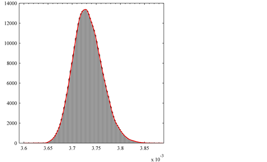
Figure 5. Density function  for
for .
.
Finally, as shown in our table of densities, the trace can be further investigated by considering the Gamma random matrix, of which the Wishart is only a special case.
References
- Tourneret, J.Y., Ferrari, A. and Letac, G. (2005) The Non-Central Wishart Distribution: Properties and Application to Speckle Imaging. 2005 IEEE/SP 13th Workshop on Statistical Signal Processing, Novosibirsk, 17-20 July 2005, 924-929.
- Díaz-García, J.A. and Gutiérrez-Jáimez, R. (2011) On Wishart Distribution: Some Extensions. Linear Algebra and its Applications, 435, 1296-1310.
- Pham-Gia, T. and Turkkan, N.T. (2011) Distributions of Ratios: from Random Variables to Random Matrices. Open Journal of Statistics, 1, 93-104.
- Chamayou, J.F. and Wesolowski, J. (2009) Lauricella and Humbert Functions through Probabilistic Tools. Integral transforms and Special Functions, 20, 529-538. http://dx.doi.org/10.1080/10652460802645750
- Mathai, A.M. and Pederzoli, G. (1995) Hypergeometric Functions of Many Matrix Variables and Distributions of Generalized Quadratic Forms. American Journal of Mathematical and Management Sciences, 15, 343-354.
- Pham-Gia, T. and Turkkan, T.N. (1999) System Availability in a Gamma Alternating Renewal Process. Naval Research Logistics, 46, 822-844. http://dx.doi.org/10.1002/(SICI)1520-6750(199910)46:7<822::AID-NAV5>3.0.CO;2-D
- Gelfand, I.M., Kapronov, W.M. and Zelevinsky, A.V. (1991) Hypergeometric Functions, Toric Varieties and Newton Polyhedra. In: Kashiwara, I.M. and Miwa, T., Eds., ICM 90 Satellite Conference Proceedings, Springer-Verlag, Tokyo, 104-121.
- Aomoto, K. and Kita, M. (2011) Theory of Hypergeometric Functions. Springer, New York. http://dx.doi.org/10.1007/978-4-431-53938-4
- Saito, M., Sturmfels, B. and Takayama, N. (2000) Grobner Deformations of Hypergeometric Differential Equations. Springer, New York. http://dx.doi.org/10.1007/978-3-662-04112-3
- Pham-Gia, T. (2008) Exact Distribution of the Generalized Wilks’s statistic and Applications. Journal of Multivariate Analysis, 99, 1698-1716. http://dx.doi.org/10.1016/j.jmva.2008.01.021
- Muirhead, R. (1982) Aspects of Multivariate Statistical Analysis. Wiley, New York.
- Mathai, A.M. and Pillai, K.C.S. (1982) Further Results on the Trace of a Non-Central Wishart Matrix. Communications in Statistics―Theory and Methods, 11, 1077-1086. http://dx.doi.org/10.1080/03610928208828294
- Kotz, S. and Srinivasan, R. (1969) Distribution of Product and Quotient of Bessel Function Variates. Annals of the Institute of Statistical Mathematics, 21, 201-210. http://dx.doi.org/10.1007/BF02532244
- Laha, R.G. (1954) On Some Properties of the Bessel Function Distributions. Bulletin of the Calcutta Mathematical Society, 46, 59-71.
- Gupta, A.K. and Nagar, D.K. (2000) Matrix Variate Distributions. Chapman and Hall/CRC, Boca Raton.
- Anderson, T.W. (1982) An Introduction to Multivariate Statistical Analysis. John Wiley and Sons, New York.
- Mathai, A.M. (1980) Moments of the Trace of a Non-Central Wishart Matrix. Communications in Statistics―Theory and Methods, 9, 795-801.
- Ruben, J. (1962) Probability Content of Regions under Spherical Normal Distribution, IV: The Distribution of Homogeneous and Non-Homogeneous Quadratic Functions in Normal Variables. The Annals of Mathematical Statistics, 33, 542-570. http://dx.doi.org/10.1214/aoms/1177704580
- Press, S.J. (1966) Linear Combinations of Non-Central Chi-Square Variates. The Annals of Mathematical Statistics, 37, 480-487.
- Hartville, D.A. (1971) On the Distribution of Linear Combinations of Non Central Chi Squares. The Annals of Mathematical Statistics, 42, 809-811.
- Provost, S. and Ruduik, E. (1996) The Exact Distribution of Indefinite Quadratic Forms in Noncentral Normal Vectors. Annals of the Institute of Statistical Mathematics, 48, 381-394. http://dx.doi.org/10.1007/BF00054797
- Castano-Martinez, A. and Lopez-Blaquez, F. (2006) Distribution of a Sum of Weighted Non Central Chi-Square Variables. TEST, 14, 397-115.
- Kourouklis, S. and Moschopoulos, P.G. (1985) On the Distribution of the Trace of a Non-Central Wishart Matrix. Metron, 43, 85-92.
- Glueck, D.H. and Muller, K.E. (1998) On the Trace of a Wishart. Communications in Statistics―Theory and Methods, 27, 2137-2141. http://dx.doi.org/10.1080/03610929808832218
- De Waal, D.J. (1972) On the Expected Values of the Elementary Symmetric Functions of a Non-Central Wishart Matrix. The Annals of Mathematical Statistics, 43, 344-347.
- Saw, J.G. (1973) Expectation of Elementary Symmetric Functions of a Wishart Matrix. Annals of Statistics, 1, 580- 582.
- Shah, B.K. and Khatri, C.G. (1974) Proofs of Conjectures about the Expected Values of the Elementary Symmetric Functions of a Non-Central Wishart Matrix. Annals of Statistics, 2, 833-636.
- Letac, G. and Massam, H. (2004) All Invariant Moments of the Wishart Distribution. Scandinavian Journal of Statistics, 31, 295-318.
- Glaser, R.E. (1976) The Ratio of the Geometric Mean to the Arithmetic Mean from a Random Sample from a Gamma Distribution. Journal of the American Statistical Association, 71, 480-487. http://dx.doi.org/10.1080/01621459.1976.10480373
- Cheng, J., Wag, N. and Tellambura, C. (2010) Probability Density Function of Logarithmic Ratio of Arithmetic Mean to Geometric Mean for Nakagami-m Fading Power. Proceedings of the 25th Biennial Symposium on Communications, Kingston, 12-14 May 2010, 348-351. http://dx.doi.org/10.1109/BSC.2010.5472954
- Mauchly, J.W. (1940) Significance Test for Sphericity of a Normal n-Variate Distribution. The Annals of Mathematical Statistics, 11, 204-209. http://dx.doi.org/10.1214/aoms/1177731915
- Pham-Gia, T. and Turkkan, T.N. (2010) Testing Sphericity Using Small Samples. Statistics, 44, 601-616.
- Glaser, R.E. (1980) A Characterization of Bartlett’s Statistic Involving Incomplete Beta Functions. Biometrika, 67, 53- 58.
- Gleser, L. (1966) A Note on Sphericity Test. The Annals of Mathematical Statistics, 37, 464-467. http://dx.doi.org/10.1214/aoms/1177699529
- Khatri, C.G. and Srivastava, M.S. (1971) On Exact Non-Null Distributions of Likelihood Ratio Criteria for Sphericity Test and Equality of Two Covariance Matrices. Sankhyā, 33, 201-206.
- Muller, K.E. and Barton, C.N. (1989) Approximate Power for Repeated-Measures ANOVA Lacking Sphericity. Journal of the American Statistical Association, 84, 549-555.
- Mathai, A.M. and Tan, W.Y. (1977) The Non-Null Distribution of the Likelihood Ratio Criterion for Testing the Hypothesis That the Covariance Matrix Is Diagonal. Canadian Journal of Statistics, 5, 63-74.
- Krishnaiah, P.R. and Shurmann, F.J. (1974) On the Evaluation of Some Distributions That Arise in Simultaneous Tests for the Equality of the Latent Roots of the Covariance Matrix. Journal of Multivariate Analysis, 4, 265-282. http://dx.doi.org/10.1016/0047-259X(74)90033-5
- Nadler, B. (2011) On the Distribution of the Ratio of the Largest Eigenvalue to the Trace of a Wishart Matrix. Unpublished Manuscript on the Internet.
- Johnstone, I. (2001) On the Distribution of the Largest Eigenvalue in Principal Components Analysis. Annals of Statistics, 29, 295-327.
- Troskie, C.G. and Conradie, W.J. (1986) The Distribution of the Ratios of the Characteristic Roots (Condition Numbers) and Their Applications in Principal Component or Ridge Regression. Linear Algebra and Its Applications, 82, 255-279. http://dx.doi.org/10.1016/0024-3795(86)90156-4
- Davis, A.W. (1972) On the Ratios of the Individual Latent Roots to the Trace of a Wishart Matrix. Journal of Multivariate Analysis, 2, 440-443. http://dx.doi.org/10.1016/0047-259X(72)90037-1
- Pham-Gia, T. and Turkkan, T.N. (2009) Testing a Covariance Matrix: Exact Null Distribution of Its Likelihood Criterion. Journal of Statistical Computation and Simulation, 79, 1331-1340.
NOTES

*Corresponding author.