Open Journal of Statistics
Vol.05 No.01(2015), Article ID:53436,10 pages
10.4236/ojs.2015.51002
Comparison of the Sampling Efficiency in Spatial Autoregressive Model
Yoshihiro Ohtsuka1, Kazuhiko Kakamu2
1Department of Economics, University of Nagasaki, Nagasaki, Japan
2Faculty of Law, Politics and Economics, Chiba University, Chiba, Japan
Email: ohtsuka@sun.ac.jp, kakamu@le.chiba-u.ac.jp
Copyright © 2015 by authors and Scientific Research Publishing Inc.
This work is licensed under the Creative Commons Attribution International License (CC BY).
http://creativecommons.org/licenses/by/4.0/


Received 29 December 2014; accepted 18 January 2015; published 22 January 2015
ABSTRACT
A random walk Metropolis-Hastings algorithm has been widely used in sampling the parameter of spatial interaction in spatial autoregressive model from a Bayesian point of view. In addition, as an alternative approach, the griddy Gibbs sampler is proposed by [1] and utilized by [2] . This paper proposes an acceptance-rejection Metropolis-Hastings algorithm as a third approach, and compares these three algorithms through Monte Carlo experiments. The experimental results show that the griddy Gibbs sampler is the most efficient algorithm among the algorithms whether the number of observations is small or not in terms of the computation time and the inefficiency factors. Moreover, it seems to work well when the size of grid is 100.
Keywords:
Acceptance-Rejection Metropolis-Hastings Algorithm, Griddy Gibbs Sampler, Markov Chain Monte Carlo (MCMC), Random Walk Metropolis-Hastings Algorithm, Spatial Autoregressive Model

1. Introduction
Spatial models have been widely used in various research fields such as physical, environmental, biological science and so on. Recently, a lot of researches are also emerging in econometrics (e.g., [3] [4] and so on), and [5] gave an excellent survey from the viewpoint of econometrics. When we focus on the estimation methods, properties of several estimation methods are studied. For example, the efficient maximum likelihood (ML) method was proposed by [6] , and [7] first formally proved that the quasi maximum likelihood estimator had the usual asymptotic properties, including  -consistency, asymptotic normality, and asymptotic efficiency. A class of moment estimators was examined by [8] and [9] . The Bayesian approach was first considered by [10] and [11] proposed a Markov chain Monte Carlo (hereafter MCMC) method to estimate the parameters of the model. We have to mention that in economic analysis typically the sample size is small, for instance, areal data such as state-level data is widely used. The maximum likelihood methods depend on their asymptotic properties while the Bayesian method does not, because the latter evaluates the posterior distributions of the parameters conditioned on the data. Therefore, it is reasonable to examine the properties of Bayesian estimators (see [12] ).
Although there are a lot of works using spatial models in a Bayesian framework, previous literature has rarely examined sampling methods for the parameter of spatial correlation. [13] proposed a random walk Metropolis- Hastings (hereafter RMH) algorithm. This method is widely used (e.g., [11] [12] [14] and so on). On the other hand, [2] applied a griddy Gibbs sampler (hereafter GGS) proposed by [1] and showed the GGS got an advantage over the RMH method from a simulated data and estimated the regional electricity demand in Japan. However, [2] has examined only one case. In this paper, we compare the properties of the GGS in the case that the number of observation is small (or large) through the Monte Carlo experiments. Desirable properties for sampling methods in the Bayesian inference are efficiency and well mixing, which yield fast convergence. In addition to these properties, computational requirements and model flexibility are important for applied econometrics. Therefore, the purpose of this paper is to investigate the properties of some sampling algorithms given several parameters of a model.
In this paper, we examine the efficiency of the existing Markov chain Monte Carlo methods for the spatial autoregressive (hereafter SAR) model which is the simplest and most commonly used model in the spatial models. Moreover, we propose an acceptance-rejection Metropolis-Hastings (hereafter ARMH) algorithm as an alternative MH algorithm, which is proposed by [15] because it is well known that the RMH is inefficient. This algorithm is widely used for the acceleration of MCMC convergence, for example, in the time series models (see [16] - [18] and so on). The advantage of this method is that the computational requirement is very small since it is irrelevant to the shape of the full conditional density. Therefore, we apply the algorithm to the SAR model.
We illustrate the properties of these algorithms using simulated data set given the three number of observations and the seven values of spatial correlation. From the results, we find that the GGS is the most efficient method whether the number of observations is small or not in terms of both the computation time and the inefficiency factors. Furthermore, we show that it is efficient when the number of grid in the GGS sampler is one hundred. These results give a benchmark of sampling the spatial correlation parameter of the models.
The rest of this paper is organized as follows. Section 2 summarizes the SAR model. Section 3 discusses the computational strategies of the MCMC methods, and reviews three sampling methods for spatial correlation parameter. Section 4 gives the Monte Carlo experiments using simulated data set and discusses the results. Finally, we summarize the results and provide concluding remarks.
2. Spatial Autoregressive (SAR) Model
Spatial autoregressive model explains the spatial spillover using a weight matrix (see [19] ). There are numerous approaches to construct the weight matrix, which plays an important role in the model. For example, those are a first order contiguity matrix, inverse distance one and so on. Among the approaches, [20] recommended the first order contiguity dummies, because they showed that the first order contiguity weight matrix identifies the true model more frequently than the other matrices through the Monte Carlo simulations. Thus, we also utilize the first order contiguity dummies as the weight matrix.
Let  be an
be an  matrix of contiguity dummies, with
  if areas
  and
and  are adjacent and
  otherwise (with
 ). We standardized the weight matrix as follows

and we define , where
  denotes the spatial weight on the
  -th unit with respect to the
  -th unit. Note that we have
  for all
 .
.
Next, let  and
and  be a dependent variable and a
  vector of covariates on the
  th unit for
 , respectively. Then, the SAR model conditioned on the parameters
 ,
,  ,
,  is written as follows:
 (1)
(1)
where  and
and  indicates the spatial correlation, and the variance of the disturbance term, respectively. As is shown in [21] , we know that
  amd
amd , where
  and
and  denote the minimum and maximum eigenvalue of
 , since we standardize the weight matrix like
 . Thus, we restrict
  to
to .
.
Then the likelihood function of the model (1) is given as follows:
 (2)
(2)
where ,
,  ,
,  ,
,  , and
, and  is an
is an  unit matrix.
3. Posterior Analysis and Simulation
3.1. Joint Posterior Distribution
Since we adopt the Bayesian approach, we complete the model by specifying the prior distribution over the parameters. We use the following independent prior distribution:

Given a prior density  and the likelihood function given in (2), the joint posterior distribution can be expressed as
 (3)
(3)
Finally, we assume the following prior distributions:

where  denotes an inverse gamma distribution with scale and shape parameters
  and
and .
.
Since the joint posterior distribution is given by (3), we can now adopt the MCMC method. The Markov chain sampling scheme can be constructed from the full conditional distributions of ,
,  and
and .
.
3.2. Sampling 
From (3), the full conditional distribution of  is written as
 (4)
(4)
As it is difficult to sample from the standard distribution, we examine three approaches for sampling . First, we introduce the GGS, which is applied by [2] . Second, we overview the RMH algorithm, which is extended by [13] . Finally, we propose an ARMH algorithm. These sampling methods are summarized in the following.
3.2.1. Griddy Gibbs Sampler
The GGS was proposed by [1] . This sampling algorithm approximates a cumulative distribution function of the full conditional distribution by each kernel function over a grid of points and uses a numerical integration method, and is sampling method from the full conditional distribution by using the inverse transform method. Let the grid be as follows

and , which is centered in the interval
 . Then, the full conditional distribution in the interval
  is approximated as follows

Thus, we select the grid  with probabilities,

Finally, we sample  from the uniform
 . [22] stated that the choice of the grid of points has to be made carefully and constitute the main difficulty in applying GGS. In this paper, we select the equal interval among
  as in [1] . Then, our numerical experiments examines to choice the size of grid for estimating the spatial correlation.
3.2.2. Random Walk Metropolis-Hastings Algorithm
The RMH method is a simple algorithm because it needs the previous value and a random walk process such as , where
  is the parameter of the previous sampling, and
  denotes the tuning para- meter, respectively. Therefore, the following Metropolis step is used: Sample
  from
from

where  is the tuning parameter. In the numerical example below, we select the tuning parameter such that the acceptance rate lies between 0.4 and 0.6 (see [13] ). Next, we evaluate the acceptance probability

And finally set  with probability
 , otherwise
 . The proposal value of
  is not truncated to the interval
  because the constraint is part of the target density. Thus, if the proposed value of
  is not within the interval, the conditional posterior is zero, and the proposal value is rejected with probability one (see [23] ). It is well known that the method is not efficient because the convergence is slow for using the previous sampled parameter.
3.2.3. Acceptance-Rejection Metropolis-Hastings Algorithm
An acceptance-rejection Metropolis-Hastings (ARMH) algorithm method was proposed by [15] . This algorithm samples the parameter using the AR and MH steps. Suppose that there is a candidate function  such that it is possible to sample directly from
  by some known method. Then, the AR step proceeds as follows. We sampling the parameter from the candidate function
 , and accepts the candidate draw with probability
 . This step is iterated until the candidate draw is accepted.
Next, suppose the candidate  is produced from above AR step. The MH part proceeds as follows. We calculate the acceptance probability,
  as following:
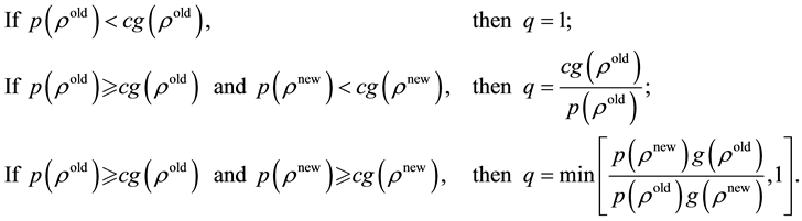
In this step, the candidate draw is accepted with probability  and rejected with probability
 . If the draw is rejected, the previously sampled value is sampled again. If
  is small, the probability of sampling the same value consecutively is high, causing high autocorrelation across sample values (see [24] ). Hence, we should also make
  as close to one as possible.
The advantage of this method is that it is free to functional form which differs from the GGS and RMH. In this paper, in order to construct the candidate function, we utilize the result of [7] , which showed the consistency and asymptotic normality of quasi-ML estimators of model parameters, to the candidate density. Then, we construct the candidate density  as an approximation to the the conditional posterior density by omitting the determinant
  as follows:
 (5)
(5)
where  and
and . Thus we sample
  from the distribution, and apply the ARMH algorithm.
3.3. Sampling Other Parameters
The full conditional distributions of  and
and  are
are

where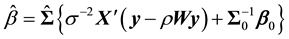 ,
,  ,
,  , and
, and . These parameters are easily sampled from the Gibbs sampler (see [25] ).
4. Comparison of MCMC Methods
4.1. Measures of Efficiency for Comparison
In this section, we examine the properties of three MCMC methods by simulated data sets. Desirable properties for sampling methods in MCMC are efficiency and well mixing, which yield fast convergence. [17] compared from the view point of acceptance rate in the AR and MH step. [26] [27] evaluated the efficiency of sampling methods, comparing the inefficiency factor and time of MCMC simulation. Following previous literatures, we also compare inefficiency factor and computational time.
The inefficiency factor is defined as  where
where  is the sample autocorrelation at lag
  calcu-
lated from the sampled values. It is used to measure how well the chain mixes and is the ratio of the numerical variance of the sample posterior mean to the variance of the sample mean from the hypothetical uncorrelated draws (see [28] ).
4.2. Data Generating Process and Estimation Procedures
We now explain the simulated data for an experiment. First, we give the weight matrix as an exogenous variable. We construct the spatial weight matrix  as follows: 1) generate
  for
for  from Bernoulli distribution with a probability of success 0.3, 2) set
  for
for  and
and  for
for , and 3) compute
  for all
 ,
, . Next, for the independent variables
 , we take the standard normal variates and set the
 , which are
  covariate matrices.
Given ,
,  ,
,  , and
, and , the true data generating process is as follows:
 (6)
(6)
where the  is normally and independently distributed with
  and
and . The parameter is set to be
  and
and , respectively. The parameters of
  for simulated data reflect the values obtained in [12] . All the results in this paper were calculated using the Ox version 5.1 (see [29] ).
The prior distributions are as follows:

We perform the MCMC procedure by generating 35,000 draws in a single sample path and discard the first 20,000 draws as the initial burn-in. For the GGS, we consider the number of grid,  for estimating the parameters.
4.3. Results of Comparison
Table 1 reports inefficiency factors by using three methods. Although there are some differences, the performances of the GGS are almost equivalent to those of the ARMH. In addition, these algorithms are more efficient than RMH. For example, from the table in , the inefficiency factors calculated by the ARMH are smaller than the other methods. However, if spatial correlation is positive strong such as
 , the value by the GGS
  has the smallest inefficiency factor. Next, we focus on the results in
 . In this case, the GGS
  perform the best for
 , respectively. In the case of
 , the values of the GGS
  and the ARMH are similar in each parameter. We can also find such similarity in sample paths and autocorrelation functions. Figure 1 shows the results of MCMC simulation in each method in the cases of
 ,
,  and
and . The figure shows that the marginal posterior densities (middle of the figure)

Table 1. Inefficiency factor of models.
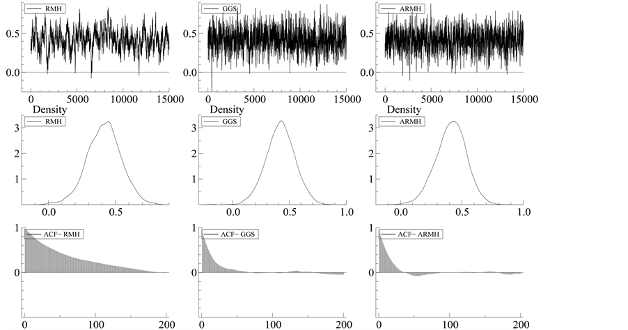
Figure 1. Sample paths, sample autocorrelation and posterior density of ,
, .
.
have similar shapes but that the sample paths (top of the figure) and autocorrelation functions (bottom of the figure) are different. From the sample paths, we can find that the ARMH and GGS mix better than the RMH. As same as the sample paths, autocorrelation functions shows the same tendency. The figure of autocorrelation indicates that both GGS and ARMH perform similarly in the autocorrelation disappear. On the contrary, the result for the RMH indicates that serious autocorrelation for parameter at large lag length.
Table 2 shows CPU time on a Pentium Core2 Duo 2.4GHz including discarded and rejected draws. For the GGS, the computation time depends on the number of grid because the increase of grid number causes the cost of computation time. In all cases, the GGS  overwhelms the others. If we focus on the case of
 , the computational time of the GGS
  are as same as those of the RMH and ARMH methods. Futhermore, if
 , the GGS needs much shorter time than the RMH and ARMH methods. Summarizing the results of inefficiency factors and computational time, if the number of observation is not only small (like
 ) but also large, then it is suitable to use the GGS. In addition, the choice of grid number affects to the computational time. In this numerical experiments, the results of selecting
  seem to work well in terms of inefficiency factors and computational time.
Table 3 shows the results with acceptance probabilities in both AR and MH parts in the ARMH. From the table, the acceptance probabilities in those part are exceed 89%. This result shows that our candidate function seems to work well, and the probabilities of sampling the same value consecutively are low. However, our ARMH algorithm does not improve the values of inefficiency factor. Thus, we think that the SAR model has the problem of identification.
Figure 2 and Table 4 depict the sample path and the correlation among the parameters in the case of ,
,  ,
,  using the GGS. From
  to
to  and
and  in the figure, the MCMC draws seem to be well mixing. In addition, correlations among these parameters are very small. On the other hand, strong correlation between
  and
and  can be found from the figure. Moreover, the correlation between
  and
and  is
is  from the table. Therefore, we assume that the spatial correlation and constant term is weakly identified.
5. Concluding Remarks
This paper reviewed the MCMC estimation procedures for sampling the spatial correlation of SAR model, and proposed the ARMH algorithm as more efficient than the RMH in order to show the property of the GGS proposed by [2] . To illustrate the differences between the estimates of three MCMC methods, we compared these algorithms by simulated data set. From the Monte Carlo experiments, we found that the GGS was the most efficient algorithm with respect to the mixing, efficiency and computational requirement of the MCMC. Moreover,
Table 2. Time of convergence.
Note: Time denotes CPU time on a Pentium Core2 Duo, including discarded and rejected draws.
Table 3. Acceptance probability of the ARMH methods.
Table 4. Correlation of parameters.
Note: True parameter is 0.9. The number of observation set to be 100.
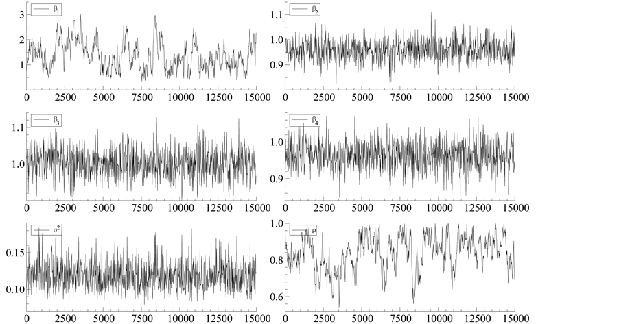
Figure 2. Sample paths of SAR model with GGS ( ,
,  ,
, ).
).
the results of selecting  seem to work well in terms of inefficiency factors and computational time. Therefore, the GGS is beneficial algorithm for estimating the spatial parameter as same as the result of [22] .
Finally, we will state our remaining issues. In this paper, we found that the GGS was the most efficient algorithm in sampling the intensity of spatial interaction. On the other hand, we showed the problem of the SAR model such that the spatial correlation and constant term was weakly identified. Thus, we have to construct the model which is identified, or appropriate algorithm to sample the intensity of spatial interaction. Furthermore, we found that the number of grids is appropriate when . In this paper, we could not derive the theoretical reason why
  was appropriate number of grids, that was, we only showed the results of Monte Carlo experiments. However, it is important to know the properties of the existing sampling methods, though research on the convergence of the GGS algorithm has never been examined. We think that, in this respect, our experiment gives the benchmark in applied econometrics.
Acknowledgements
We gratefully acknowledge helpful discussions and suggestions with Toshiaki Watanabe on several points in the paper. Mototsugu Fukushige gave insightful comments and suggestions when we made a presentation at Japan Association for Applied Economics in June, 2009. This research was partially supported by KAKENHI # 25245035 for K. Kakamu.
Cite this paper
YoshihiroOhtsuka,KazuhikoKakamu, (2015) Comparison of the Sampling Efficiency in Spatial Autoregressive Model. Open Journal of Statistics,05,10-20. doi: 10.4236/ojs.2015.51002
References
- 1. Ritter, C. and Tanner, M. (1992) Facilitating the Gibbs Sampler: The Gibbs Stopper and the Griddy-Gibbs Sampler. Journal of the American Statistical Association, 87, 861-868.
http://dx.doi.org/10.1080/01621459.1992.10475289 - 2. Ohtsuka, Y. and Kakamu, K. (2009) Estimation of Electric Demand in Japan: A Bayesian Spatial Autoregressive AR(p) Approach. In: Schwartz, L.V., Ed., Inflation: Causes and Effects, Nova Science Publisher, New York, 156-178.
- 3. Anselin, L. (2003) Spatial Externalities, Spatial Multipliers, and Spatial Econometrics. International Regional Science Review, 26, 153-166.
http://dx.doi.org/10.1177/0160017602250972 - 4. Gelfand, A.E., Banerjee, S., Sirmans, C.F., Tu, Y. and Ong, S.E. (2007) Multilevel Modeling Using Spatial Processes: Application to the Singapore Housing Market. Computational Statistics and Data Analysis, 51, 3567-3579.
http://dx.doi.org/10.1080/01621459.1990.10476213 - 5. Anselin, L. (2010) Thirty Years of Spatial Econometrics. Papers in Regional Science, 89, 3-25.
http://dx.doi.org/10.1111/j.1435-5957.2010.00279.x - 6. Ord, K. (1975) Estimation Methods for Models for Spatial Interaction. Journal of the American Statistical Association, 70, 120-126.
http://dx.doi.org/10.1080/01621459.1975.10480272 - 7. Lee, L.F. (2004) Asymptotic Distributions of Quasi-Maximum Likelihood Estimators for Spatial Autoregressive Models. Econometrica, 72, 1899-1925.
http://dx.doi.org/10.1111/j.1468-0262.2004.00558.x - 8. Conley, T.G. (1999) GMM Estimation with Cross Sectional Dependence. Journal of Econometrics, 92, 1-45.
http://dx.doi.org/0.1016/S0304-4076(98)00084-0 - 9. Kelejian, H.H. and Prucha, I.R. (1999) A Generalized Moments Estimator for the Autoregressive Parameter in a Spatial Model. International Economic Review, 40, 509-533.
http://dx.doi.org/10.1111/1468-2354.00027 - 10. Anselin, L. (1980) A Note on Small Sample Properties of Estimators in A First-order Spatial Autoregressive Model. Environment and Planning A, 14, 1023-1030.
http://dx.doi.org/10.1068/a141023 - 11. LeSage, J.P. (1997) Regression Analysis of Spatial Data. The Journal of Regional Analysis and Policy, 27, 83-94.
- 12. Kakamu, K. and Wago, H. (2008) Small-Sample Properties of Panel Spatial Autoregressive Models: Comparison of the Bayesian and Maximum Likelihood Methods. Spatial Economic Analysis, 3, 305-319.
http://dx.doi.org/10.1080/17421770802353725 - 13. Holloway, G., Shankar, B. and Rahman, S. (2002) Bayesian Spatial Probit Estimation: A Primer and an Application to HYV Rice Adoption. Agricultural Economics, 27, 383-402.
http://dx.doi.org/10.1111/j.1574-0862.2002.tb00127.x - 14. Ohtsuka, Y., Oga, T. and Kakamu, K. (2010) Forecasting Electricity Demand in Japan: A Bayesian Spatial Autoregressive ARMA Approach. Computational Statistics & Data Analysis, 54, 2721-2735.
http://dx.doi.org/10.1016/j.csda.2009.06.002 - 15. Tierney, L. (1994) Markov Chains for Exploring Posterior Distributions (with Discussion). Annals of Statistics, 22, 1701-1728.
http://dx.doi.org/10.1214/aos/1176325750 - 16. Chib, S. and Greenberg, E. (1994) Bayes Inference in Regression Models with ARMA( ) Errors. Journal of Econometrics, 64, 183-206.
http://dx.doi.org/10.1016/0304-4076(94)90063-9 - 17. Watanabe, T. (2001) On Sampling the Degree-of-Freedom of Student’s-t Disturbances. Statistics & Probability Letters, 52, 177-181.
http://dx.doi.org/10.1016/S0167-7152(00)00221-2 - 18. Mitsui, H. and Watanabe, T. (2003) Bayesian Analysis of GARCH Option Pricing Models. Journal of the Japan Statistical Society (Japanese Issue), 33, 307-324.
- 19. LeSage, J.P. and Pace, R.K. (2008) Introduction to Spatial Econometrics (Statistics: A Series of Textbooks and Monographs). Chapman and Hall/CRC, London.
- 20. Stakhovych, S. and Bijmolt, T.H.A. (2009) Specification of Spatial Models: A Simulation Study on Weights Matrices. Papers in Regional Science, 88, 389-408.
http://dx.doi.org/10.1111/j.1435-5957.2008.00213.x - 21. Sun, D., Tsutakawa, R.K. and Speckman, P.L. (1999) Posterior Distribution of Hierarchical Models Using CAR(1) Distributions. Biometrika, 86, 341-350.
http://dx.doi.org/10.1093/biomet/86.2.341 - 22. Bauwens, L. and Lubrano, M. (1998) Bayesian Inference on GARCH Models Using the Gibbs Sampler. The Econometrics Journal, 1, 23-46.
http://dx.doi.org/10.1111/1368-423X.11003 - 23. Chib, S. and Greenberg, E. (1998) Analysis of Multivariate Probit Models. Biometrika, 85, 347-361.
http://dx.doi.org/10.1093/biomet/85.2.347 - 24. Chib, S. and Greenberg, E. (1995) Understanding the Metropolis-Hastings Algorithm. The American Statistician, 49, 327-335.
- 25. Gelfand, A.E. and Smith, A.F.M. (1990) Sampling-Based Approaches to Calculating Marginal Densities. Journal of the American Statistical Association, 85, 398-409.
http://dx.doi.org/10.1080/01621459.1990.10476213 - 26. Asai, M. (2005) Comparison of MCMC Methods for Estimating Stochastic Volatility Models. Computational Economics, 25, 281-301.
http://dx.doi.org/10.1007/s10614-005-2974-4 - 27. Asai, M. (2006) Comparison of MCMC Methods for Estimating GARCH Models. Journal of the Japan Statistical Society, 36, 199-212.
http://dx.doi.org/10.14490/jjss.36.199 - 28. Chib, S. (2001) Markov Chain Monte Carlo Methods: Computation and Inference. In: Heckman, J.J. and Leamer, E., Eds., Handbook of Econometrics, Elsevier, Amsterdam, 3569-3649.
- 29. Doornik, J.A. (2006) Ox: An Object Oriented Matrix Programming Language. Timberlake Consultants Press, London.