Open Journal of Statistics
Vol.4 No.5(2014), Article ID:48571,15 pages
DOI:10.4236/ojs.2014.45033
Distribution of the Sample Correlation Matrix and Applications
Thu Pham-Gia, Vartan Choulakian
Department of Mathematics and Statistics, Université de Moncton, Moncton, Canada
Email: Thu.pham-gia@umoncton.ca, Vartan.choulakian@umoncton.ca
Copyright © 2014 by authors and Scientific Research Publishing Inc.
This work is licensed under the Creative Commons Attribution International License (CC BY).
http://creativecommons.org/licenses/by/4.0/


Received 29 May 2014; revised 5 July 2014; accepted 15 July 2014
ABSTRACT
For the case where the multivariate normal population does not have null correlations, we give the exact expression of the distribution of the sample matrix of correlations R, with the sample variances acting as parameters. Also, the distribution of its determinant is established in terms of Meijer G-functions in the null-correlation case. Several numerical examples are given, and applications to the concept of system dependence in Reliability Theory are presented.
Keywords: Correlation, Normal, Determinant, Meijer G-Function, No-Correlation, Dependence, Component, Formatting, Style, Styling, Insert

1. Introduction
The correlation matrix plays an important role in multivariate analysis since by itself it captures the pairwise degrees of relationship between different components of a random vector. Its presence is very visible in Principal Component Analysis and Factor Analysis, where in general, it gives results different from those obtained with the covariance matrix. Also, as a test criterion, it is used to test the independence of variables, or subsets of variables ([1] , p. 407).
In a normal distribution context, when the population correlation matrix , the identity matrix, or equivalently,
the population covariance matrix
, the identity matrix, or equivalently,
the population covariance matrix
 is diagonal, i.e.
 , the distribution of the sample correlation
matrix R is relatively easy to compute, and its determinant has a distribution that
can be expressed as a Meijer G-function distribution. But when
, the distribution of the sample correlation
matrix R is relatively easy to compute, and its determinant has a distribution that
can be expressed as a Meijer G-function distribution. But when
 no expression for the density of R is presently available in the literature, and
the distribution of its determinant is still unknown, in spite of efforts made by
several researchers. We will provide here the closed form expression of the distribution
of R, with the sample variances as parameters, hence complementing a result presented
by Fisher in [2] .
no expression for the density of R is presently available in the literature, and
the distribution of its determinant is still unknown, in spite of efforts made by
several researchers. We will provide here the closed form expression of the distribution
of R, with the sample variances as parameters, hence complementing a result presented
by Fisher in [2] .
As explained in [3] , for a random matrix, there
are at least three distributions of interest, its “entries distribution” which gives
the joint distribution of its matrix entries, its “determinant distribution” and
its “latent roots distribution”. We will consider the first two only and note that,
quite often, the first distribution is also expressed in terms of the determinant,
and can lead to some confusion. In Section 2 we recall some results related to the
case where , and establish the new exact
expression of the density of R, with the sample variances
, and establish the new exact
expression of the density of R, with the sample variances
 as parameters, denoted
 . In Section 3, some simulation
results are given. The distribution of
. In Section 3, some simulation
results are given. The distribution of , the determinant
of R, is given in Section 4 for
, the determinant
of R, is given in Section 4 for . Applications of the above
results to the concept of dependence within a multi-component system are given in
Section 5. Numerical examples are given throughout the latter part of the paper
to illustrate the results.
. Applications of the above
results to the concept of dependence within a multi-component system are given in
Section 5. Numerical examples are given throughout the latter part of the paper
to illustrate the results.
2. Case of the Population Correlation Matrix Not Being Identity
2.1. Covariance and Correlation Matrices
Let us consider a random vector X with mean
 and covariance matrix
 , of the form of
a (p × p) symmetric positive definite random matrix
, of the form of
a (p × p) symmetric positive definite random matrix
of pairwise covariances between components in the matrix.
We obtain the population correlation matrix
 by diving each
 by
by . Then
 , where
 , is symmetrical, with diagonals
 ,
,
 , i.e.
 .
.
For a sample of size n of observations from , the sample mean
 and the “adjusted sample covariance” matrix
 , (1)
, (1)
(or matrix of sums of squares and products, ) are independent,
with the latter having a Wishart distribution
) are independent,
with the latter having a Wishart distribution . Similarly, the correlation
matrix
. Similarly, the correlation
matrix
 is obtained from S by using the relations:
 , or
, or , where
 . We also have the relation
between determinants:
. We also have the relation
between determinants: , and, similarly,
 .
.
It is noted that by considering the usual sample covariance matrix , which is
 , we have the relation
 , between the
two diagonal elements, but the sample correlation matrix is the same.
, between the
two diagonal elements, but the sample correlation matrix is the same.
The
 coefficients
 are (marginally) distributed independently of both the sample and population means
[2] . It is to be noticed that while R can always be defined
from S, the reverse is not true since S has
are (marginally) distributed independently of both the sample and population means
[2] . It is to be noticed that while R can always be defined
from S, the reverse is not true since S has
 independent parameters. This fact explains the differences between results when
either R or S is used.
independent parameters. This fact explains the differences between results when
either R or S is used.
In the bivariate case, Hotelling’s expression [4]
clearly shows that the density of r depends only on the population correlation coefficient
 and the sample size n (see Section 4.3) and we will see that, similarly, the density
of the sample correlation matrix, with the sample variances as parameters, is dependent
on the population variances and the sample size. However,
and the sample size n (see Section 4.3) and we will see that, similarly, the density
of the sample correlation matrix, with the sample variances as parameters, is dependent
on the population variances and the sample size. However,
 are biased estimators of
 , and Olkin and
Pratt [5] have suggested using the modified estimator
, and Olkin and
Pratt [5] have suggested using the modified estimator , with a table of corrective multipliers for
 for convenience.
2.2. Some Related Work
Several efforts have been carried out in the past to obtain the exact form of the
density of R for the general case, where ,
,
 and
and . For example,
Joarder and Ali [6] derived the distribution of
R for a class of elliptical models. Ali, Fraser and Lee
[7] , starting from the identity correlation matrix case, derived the
density for the general case when
. For example,
Joarder and Ali [6] derived the distribution of
R for a class of elliptical models. Ali, Fraser and Lee
[7] , starting from the identity correlation matrix case, derived the
density for the general case when , again by modulating the likelihood
ratio to obtain a density of R containing the function
, again by modulating the likelihood
ratio to obtain a density of R containing the function , already used by Fraser ([8]
, p. 196) in the bivariate case. But here,
, already used by Fraser ([8]
, p. 196) in the bivariate case. But here,
 , expressed as an infinite series, has a much
more complicated expression. Schott ([9] , p. 408),
using
, expressed as an infinite series, has a much
more complicated expression. Schott ([9] , p. 408),
using , gives for a first-order approximation for
R and the expression of
, gives for a first-order approximation for
R and the expression of , and Kollo and Ruul
[10] , also using
, and Kollo and Ruul
[10] , also using , presented a general
method for approximating the density of R through another multivariate density,
possibly one of higher dimension. Finally, Farrell ([11]
, p. 177) has approached the problem using exterior differential forms. However,
no explicit expression for the density of R is given in any of these works, and
the question rightly raised is whether that such an expression really exists.
, presented a general
method for approximating the density of R through another multivariate density,
possibly one of higher dimension. Finally, Farrell ([11]
, p. 177) has approached the problem using exterior differential forms. However,
no explicit expression for the density of R is given in any of these works, and
the question rightly raised is whether that such an expression really exists.
2.3. Some New Results
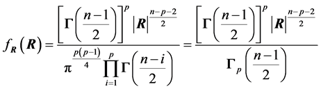
We begin with the case of . Then it can be easily established that
the density of R is ([12] , p. 107):
. Then it can be easily established that
the density of R is ([12] , p. 107):
 (2)
(2)
By showing that the joint density of the diagonal elements
 with R, denoted
 , can be factorized into the
product of two densities,
, can be factorized into the
product of two densities,
 and
and , which has expression
(2) above.
, which has expression
(2) above.
 and R are hence independent.
We can also show that (2) is a density, i.e. it integrates to 1 within its definition domain, by using the approach given in Mathai and Haubold ([13] , p. 421), based on matrix decomposition.
In what follows, following Kshirsagar’s approach [14]
, which itself is a variation of Fisher’s
[2] original
method, we establish first the expression of a similar joint distribution, when
 is not diagonal.
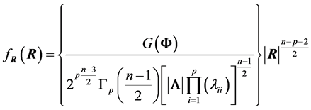
THEOREM 1:
Let
 , where we suppose that the population correlation
 and its inverse
 has
has
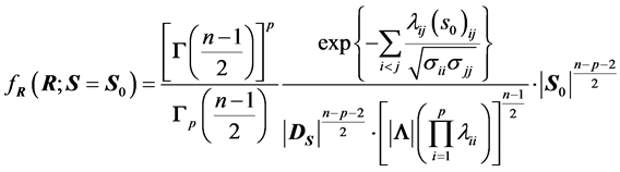
 as its diagonal elements. Then the correlation matrix R of a random sample of n
observations has its distribution given by:
as its diagonal elements. Then the correlation matrix R of a random sample of n
observations has its distribution given by:
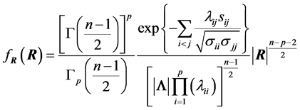 , (3)
, (3)
where , with the sample covariance
 ,
,
 , serving as parameters.
PROOF: Let us consider the “adjusted sample covariance matrix” S, given by (1).
We know that

 , with density:
 with C being an appropriate constant.
Our objective is to find the joint density of R with a set of variables
 so that the density of R can be obtained by integrating out the variables
 .
.
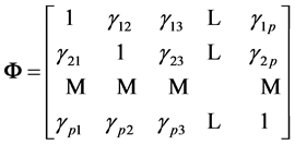
Let
 be the inverse of
 , the (population)
matrix of correlations, with diagonals
, the (population)
matrix of correlations, with diagonals ,
,
 and non-diagonals
 ,
,
 ,
, . We first transform
the
. We first transform
the
 variables
 ,
,
 , into
 . Since the diagonal
 remain unchanged, the Jacobian of the transformation from S to
 is then
 and the new joint density is:

where
 and
and .
.
We set
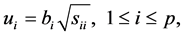 (4)
(4)
with , and form the symmetric matrix
 , (5)
, (5)
where , which depends on S.
The joint density of
 and R is now:
 .
.
R and
 are independent only if the above expression can be expressed as the product
 , which is not the case since
 contains
 .
.
To integrate out the vector , we set
 ,
,
(This integral is denoted
 by Fisher
[2] , and by
by Fisher
[2] , and by
 by Kshirsagar [14] who used the notation
 and, in both instances, was left non-computed).
Hence, if
 is constant, as in the case when
 , R would have density
 , (6)
, (6)
with , being the p-gamma function. However, in
the general case this is not true.
, being the p-gamma function. However, in
the general case this is not true.
Consider the quadratic form:
 and
and
 .
.
Changing to , we have
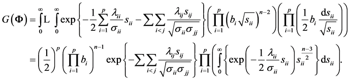
Since each integral is a gamma density in , with value
 , we obtain
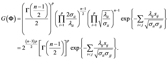
 contains all non-diagonal entries of the sample
covariance matrix, and depends on S. We now obtain from (6) expression (3) of Theorem
1. Here, the off-diagonal sample covariance,
contains all non-diagonal entries of the sample
covariance matrix, and depends on S. We now obtain from (6) expression (3) of Theorem
1. Here, the off-diagonal sample covariance,
 , serve as parameters of this density.
QED.
Alternately, using the corresponding correlation coefficients, we have:
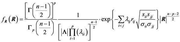 , (7)
, (7)
REMARKS:
1) For
 our results given above should reduce to known results, and they do. Indeed, since
we now have
our results given above should reduce to known results, and they do. Indeed, since
we now have

 .
.
Hence,
as in (2) since we now have .
.
Here, only the value of p needs to be known and this explains why expression (2) depends only on n and p. Also, as pointed out by Muirhead ([15] , p. 148), if we do not suppose normality, the same results can be obtained under some hypothesis.
2) Expression (3) can be interpreted as the density of R when
 are known, and
 , is a set of constant sample
covariances. But when this set is considered as a random vector, with a certain
distribution,
, is a set of constant sample
covariances. But when this set is considered as a random vector, with a certain
distribution,
 is called mixture distribution, defined in
two steps:
is called mixture distribution, defined in
two steps:
a)
 has an (known or unknown) distribution
 , i.e.
 .
.
b) (R; ) has the density given by (3), denoted
 .
.
The distribution of R is then , where * denotes the mixture
operation.
, where * denotes the mixture
operation.
However, a closed form for this mixture is often difficult to obtain.
Alternately,
 could be
 , with
 being the density of the diagonal sample variances

and off-diagonal sample correlations,
 while
while
 is given by (7).
3) We have, using (3), and the relation
 the following equivalent expression, where
 :
:
 . (8)
. (8)
Expression (8) gives the positive numerical value of
 upon knowledge of the value of S. It will serve to set up simulation computations
in Section 3. However, it also shows that
upon knowledge of the value of S. It will serve to set up simulation computations
in Section 3. However, it also shows that
 can be defined with S, and when S has a certain distribution the values of
 are completely determined with that distribution. This highlights again the fact
that, in statistics, using R or S can lead to different results, as mentioned previously.
are completely determined with that distribution. This highlights again the fact
that, in statistics, using R or S can lead to different results, as mentioned previously.
2.4. Other Known Results
1) The distribution of the sample coefficient of correlation in the bivariate normal
case can be determined fairly directly when integrating out
 and
and , and this fact is mentioned explicitly by
Fisher ([2]
, p. 4), who stated: “This, however, is not a feasible path for more than two variables.”
In the bivariate case,
, and this fact is mentioned explicitly by
Fisher ([2]
, p. 4), who stated: “This, however, is not a feasible path for more than two variables.”
In the bivariate case,
 , and has been well-studied by several researchers,
using different approaches and, as early as 1915, Fisher
[16] gave its density as:
, and has been well-studied by several researchers,
using different approaches and, as early as 1915, Fisher
[16] gave its density as:
 (9)
(9)
Using geometric arguments, with
 being the population coefficient of correlation. We refer to ([17]
, p. 524-534) for more details on the derivation of the above expression. Other
equivalent expressions, reportedly as numerous as 52, were obtained by other researchers,
such as Hotelling [4] , Sawkins [18] , Ali et al. [7]
.
being the population coefficient of correlation. We refer to ([17]
, p. 524-534) for more details on the derivation of the above expression. Other
equivalent expressions, reportedly as numerous as 52, were obtained by other researchers,
such as Hotelling [4] , Sawkins [18] , Ali et al. [7]
.
2) Using Equation (3) on the sample correlation matrix , obtained from the
sample covariance matrix
, obtained from the
sample covariance matrix
 Together with p = 2, we can also arrive at
one of these forms (see also Section 4.3, where the determinant of R provides a
more direct approach).
Together with p = 2, we can also arrive at
one of these forms (see also Section 4.3, where the determinant of R provides a
more direct approach).
3) Although Fisher [2] did not give the explicit form of the
integral
 above, he included several interesting results on
 , as a function of the sample
size n and coefficients
, as a function of the sample
size n and coefficients . For example, in the case all
 ,
,
 , the generalized volume in the p(p −
1)/2-dimension space of the region of integration for rij is found to
be a function of p, having a maximum at p = 6. In the case all
, the generalized volume in the p(p −
1)/2-dimension space of the region of integration for rij is found to
be a function of p, having a maximum at p = 6. In the case all , the expressions
of the partial derivatives of Log
, the expressions
of the partial derivatives of Log w.r.t.
 can be obtained, and so are the mixed derivatives.
For the case n = 2, and p = 3,
 has an interesting geometrical interpretation
as
has an interesting geometrical interpretation
as , where V = generalized volume defined by
 and D is the volume defined by the p unit vectors in a transformation where
 are the cosines of the angles between pairs of edges.
3. Some Computation and Simulation Results
3.1. Simulations Related to R
A matrix equation such as (3) can be difficult to visualize numerically, especially
when the dimensions are high, i.e. . Ideally, to illustrate (7), a figure
giving
. Ideally, to illustrate (7), a figure
giving
 in function of the matrix R itself is most informative, but, naturally, impossible
to obtain. One question we can investigate is how the values of
in function of the matrix R itself is most informative, but, naturally, impossible
to obtain. One question we can investigate is how the values of
 distributed, for a normal model
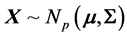 ? Simulation using (8)
can provide some information on this distribution in some specific cases. For example,
we can start from the (4 × 4) population covariance matrix
? Simulation using (8)
can provide some information on this distribution in some specific cases. For example,
we can start from the (4 × 4) population covariance matrix
 taken from our analysis of Fisher’s iris data [19] . It concerns the Setosa iris variety, with x1
= sepal length, x2 = sepal with, x3 = petal length and x4
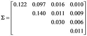
= petal width. It gives the population correlation matrix
taken from our analysis of Fisher’s iris data [19] . It concerns the Setosa iris variety, with x1
= sepal length, x2 = sepal with, x3 = petal length and x4
= petal width. It gives the population correlation matrix
 where all
 . We generate 10,000
samples of 100 observations each from
. We generate 10,000
samples of 100 observations each from , which give 10,000 values
of the covariance matrix S, which, in turn, give matrix values for R, scalar values
for
, which give 10,000 values
of the covariance matrix S, which, in turn, give matrix values for R, scalar values
for
 and, finally, positive scalar values for
 , as given by (8). Recall
that for X normal S has a Wishart distribution
, as given by (8). Recall
that for X normal S has a Wishart distribution . Figure 1
gives the corresponding histogram, which shows that values of W are distributed
along a unimodal density, denoted by
. Figure 1
gives the corresponding histogram, which shows that values of W are distributed
along a unimodal density, denoted by , with a very small variation
interval, i.e. most of its values are concentrated around the mode.
, with a very small variation
interval, i.e. most of its values are concentrated around the mode.
Note: A special approach to graphing distributions of covariance matrices, using the principle of decomposing a matrix into scale parameters and correlations, is presented in: Tokuda, T., Goodrich, B., Van Mechelen, I., Gelman, A. and Tuerlinckx, F., Visualizing Distributions of Covariance Matrices (Document on the Internet).
It is also mentioned there that for the Inverted Wishart case, with
 degrees of freedom, then
 where
where
 is the i-th principal sub-matrix of R, obtained by removing row and column i (p.
12).
is the i-th principal sub-matrix of R, obtained by removing row and column i (p.
12).
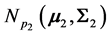
3.2. Simulations Related to

Similarly, the same application above gives the approximate simulated distribution
of
 presented in Figure 2. We can see that it is a
unimodal density which depends on the correlation coefficients
presented in Figure 2. We can see that it is a
unimodal density which depends on the correlation coefficients .
.
Using expression (7), which exhibits explicitely rij, and replacing rij
by the corrected value the unbiased estimator
of
the unbiased estimator
of , we obtain
 . However, since an unbiased estimator
of
. However, since an unbiased estimator
of
 is still to be found we cannot use neither
 nor
nor
 as point-estimate of
 . Figure 2
gives the simulated distributions of
. Figure 2
gives the simulated distributions of
 and of
 . We can see that the two approximate densities
are different, and the density of
. We can see that the two approximate densities
are different, and the density of
 has higher mean and median, resulting in a shift to the right. But, again, the two
variation intervals are very small.
has higher mean and median, resulting in a shift to the right. But, again, the two
variation intervals are very small.
3.3. Expression of

In the proof of Theorem 1, we have established that
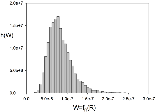
Figure 1. Simulated density
of .
.
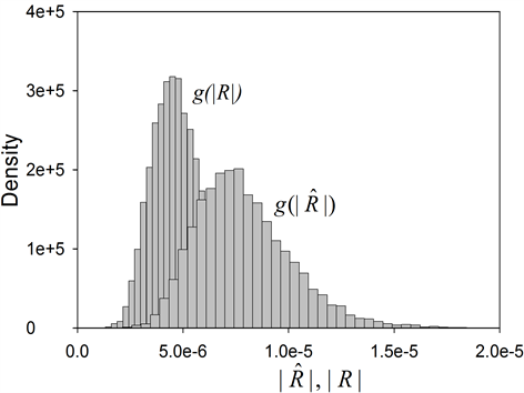
Figure 2.
Simulated densities of
 and
and .
.

Using the above matrix , for a simulated sample,
say
, for a simulated sample,
say
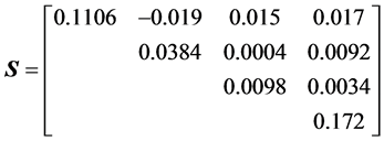 we compute directly the left side by numerical integration,
and the right side by using the algebraic expression. The results are extremely
close to each other, with both around the numerical value 1.238523012 × 10⁵.
we compute directly the left side by numerical integration,
and the right side by using the algebraic expression. The results are extremely
close to each other, with both around the numerical value 1.238523012 × 10⁵.
4. Distribution of , the Determinant of R
First, let det(R) be denoted by . In this case
 , this distribution is very complex
and no related result is known when
, this distribution is very complex
and no related result is known when . Nagar and Castaneda
[20] , for example, established some results in the general case,
for p = 2.
. Nagar and Castaneda
[20] , for example, established some results in the general case,
for p = 2.
Theoretically, we can obtain the density of
 from (3) by applying the transformation
 , with differential
 , but the expression obtained quickly
becomes intractable. Only in the case of
, but the expression obtained quickly
becomes intractable. Only in the case of
 that we can derive some analytical results on
 , as presented in the next section.
Gupta and Nagar [21] established some results
for the case of a mixture of normal models, but again under the hypothesis of
, as presented in the next section.
Gupta and Nagar [21] established some results
for the case of a mixture of normal models, but again under the hypothesis of .
.
4.1. Density of the Determinant

When considering Meijer G-functions and their extensions, Fox’s H-functions [22] , for
 the density of
 can be expressed in closed forms, as are those of other related multivariate statistics
[23] . Let us recall that the Meijer
function
can be expressed in closed forms, as are those of other related multivariate statistics
[23] . Let us recall that the Meijer
function , and the Fox function
 , are defined as follows:
 is the integral along the complex contour L of a
rational expression of Gamma functions
is the integral along the complex contour L of a
rational expression of Gamma functions
 (10)
(10)
It is a special case, when

 , of Fox’s H-function, defined as:
 .
.
Under some fairly general conditions on the poles of the gamma functions in the numerator, the above integrals exist.
THEOREM 2: When , for a random sample of size n from
 , the density of
 depends only on n and p:
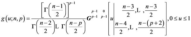 . (11)
PROOF:
From (2) the moments of order t of
 are:
are:
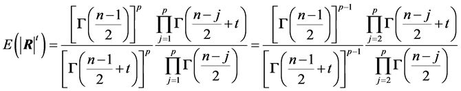 , (12)
 , which is a product of moments of order t of independent beta
variables. Upon identification of (12) with these products, we can see that
, which is a product of moments of order t of independent beta
variables. Upon identification of (12) with these products, we can see that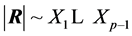 , with
 , with
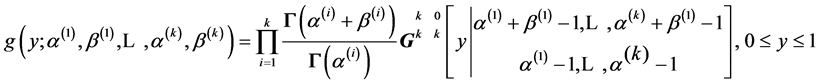
 . Using
[23] the product of k independent betas,
. Using
[23] the product of k independent betas,
 , has as density
Hence, we have here, the density of
 as:
as:
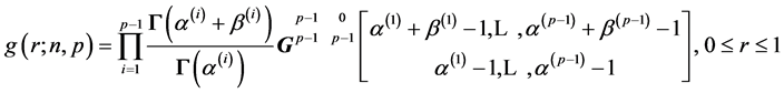 where
where ,
,
 ,
,
 ,
,
 and
and ,
, .
.
And, hence, we obtain:
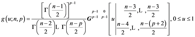 (13)
(13)
QED.
The density of
 can easily be computed and graphed, and percentiles of
 can be determined numerically. For example, for p = 4, n = 8. The 2.5th
and 97.5th percentiles can be found to be 0.04697 and 0.7719 respectively.
can be determined numerically. For example, for p = 4, n = 8. The 2.5th
and 97.5th percentiles can be found to be 0.04697 and 0.7719 respectively.
4.2. Product and Ratio
Let
 and
and
 be two independent correlation matrices, obtained from 2 populations, each with
zero population correlation coefficients. The determinant of their product is also
a G-function distribution, and its density can be obtained. This result is among
those which extend relations obtained in the univariate case by Pham-Gia and Turkkan
[24] , and also has potential applications in
several domains.
be two independent correlation matrices, obtained from 2 populations, each with
zero population correlation coefficients. The determinant of their product is also
a G-function distribution, and its density can be obtained. This result is among
those which extend relations obtained in the univariate case by Pham-Gia and Turkkan
[24] , and also has potential applications in
several domains.
THEOREM 3: Let
 and
and
 be two independent random samples from
 and
and
 respectively, both
 being diagonal. Then the determinant
 of the product
 of the two correlation matrices
 and
and
 has density:
 , (14)
where
 and
and .
.
PROOF: Immediate by using multiplication of G-densities presented in [23] .
QED.
Figure 3 shows the density of , for
, for ,
,
 and
and ,
, .
.
Using again results presented in [23]
we can similarly derive the density of the ratio
 in terms of G-functions. Its expression is not given here to save space but is available
upon request.
in terms of G-functions. Its expression is not given here to save space but is available
upon request.
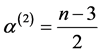
4.3. Particular Cases
1) Bivariate normal case: a) for the bivariate case we have , and when
 is zero, we have from (11) the density of
 as
as
 which is the G-function form of the beta
 . Hence, the distribution
of
. Hence, the distribution
of
 is:
is: ,
,
 , and the density of r is:
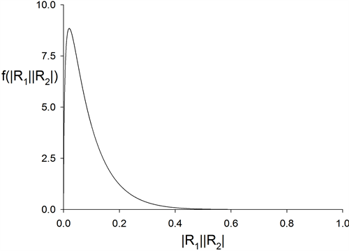
Figure 3. Density of product of independent correlation determinants.
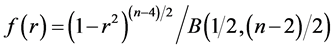 , (15)
for . Testing
 is much simpler when using Student’s t-distribution,
 , and is covered in most textbooks.
Pitman [25] has given an interesting distribution-free
test when .
.
2) When
 Hotelling ([4] ) gave the density of
 as:
as:
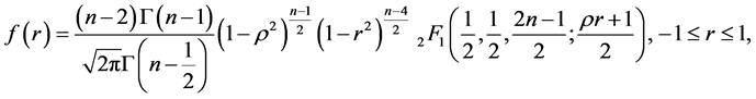 (16)
(16)
where
 is Gauss hypergeometric function with parameters
 and c.
3) Mixture of Normal Distributions: With X coming now from the mixture: ,
,
 , Gupta and Nagar [21]
consider
, Gupta and Nagar [21]
consider , and give the density
of W in terms of Meijer G-functions, but for the case
, and give the density
of W in terms of Meijer G-functions, but for the case
 only. The complicated form of this density contains the hypergeometric function
 , as expected.
For the bivariate case, Nagar and Castaneda [20]
established the density of r and gave its expression for both cases,
 and
and . In the first case
the density of r, when only one population is considered, reduces to the expression
obtained by Hotelling [4] above.
. In the first case
the density of r, when only one population is considered, reduces to the expression
obtained by Hotelling [4] above.
5. Dependence between Components of a Random Vector
5.1. Dependence and

Correlation is useful in multiple regression analysis, where it is strongly related
to collinearity. As an example of how individual correlation coefficients are used
in regression, the variance inflation factor (VIF), well adopted now in several
statistical softwares, measures how much the variance of a coefficient is increased
by collinearity, or in other words, how much of the variation in one independent
variable is explained by the others. For the j-th variable,
 is the j-th diagonal element of
 . We know that it equals
 , with
 being the multiple correlation of the j-th variable regressed on the remaining
 others.
When all correlation measures are considered together, measuring intercorrelation
by a single number has been approached in different ways by various authors. Either
the value of
 or those of its latent roots can be used. Rencher ([26]
, p. 21) mentions six of these measures, among them
or those of its latent roots can be used. Rencher ([26]
, p. 21) mentions six of these measures, among them , where
 is an observed value of R, and takes the value 1 if the variables are independent,
and 0 if there is an exact linear dependence. But since the exact distribution of
R is not available this sample measure is rather of descriptive type and no formal
inferential process has really been developed.
is an observed value of R, and takes the value 1 if the variables are independent,
and 0 if there is an exact linear dependence. But since the exact distribution of
R is not available this sample measure is rather of descriptive type and no formal
inferential process has really been developed.
Although the notion of independence between different components of a system is of widespread use in the study of the system structure, reliability and performance, its complement, the notion of dependence has been a difficult one to deal with. There are several dependence concepts, as explained by Jogdev [27] , but using the covariance matrix between different components in a joint distribution remains probably the most direct approach. Other more theoretical approaches, are related to the relations between marginal and joint distributions, and Joe [28] can be consulted on these approaches. Still, other aspects of dependence are explored in Bertail et al. [29] . But two random variables can have zero correlation while being dependent. Hence, no-correlation and independence are two different concepts, as pointed out in Drouet Mari and Kotz [30] . Furthermore, for two independent events, the product of their probabilities gives the probability of the intersection event, which is not necessarily the case for two non-correlated events. Fortunately, these two concepts are equivalent, when the underlying population is supposed normal, a hypothesis that we will suppose in this section.
5.2. Inner Dependence of a System
When considering only two variables, several measures of dependence have also been
suggested in the literature (Lancaster [31] ),
and especially in system reliability (Hoyland and Rausand
[32] ), but a joint measure of the degree of dependence between several
components of a random vector, or within a system , or inner dependence of
 , denoted by
 , is still missing. We approach
this dependence concept here by way of the correlation matrix, where a single measure
attached to it would reflect the overall degree of dependence. This concept has
been presented first in Bekker, Roux and Pham-Gia [33]
, to which we refer for more details. It is defined as
, is still missing. We approach
this dependence concept here by way of the correlation matrix, where a single measure
attached to it would reflect the overall degree of dependence. This concept has
been presented first in Bekker, Roux and Pham-Gia [33]
, to which we refer for more details. It is defined as , with
 . The measure of independence
within the system is then
. The measure of independence
within the system is then
 , estimated by
 , where
 is a point estimation of
 based on R, the correlation matrix associated with a sample of n observations of
the p-component system. In the general case this estimation question is still unresolved,
except for the binormal case,
based on R, the correlation matrix associated with a sample of n observations of
the p-component system. In the general case this estimation question is still unresolved,
except for the binormal case, . We then have
 , and
, and , where
 is the coefficient of correlation with its estimation well known, depending on either
 is supposed to be zero or not. The associated sample measure being
 , it is of interest to
study the distribution of the sample inner dependence
, it is of interest to
study the distribution of the sample inner dependence , based on a sample of n observations
of the system.
, based on a sample of n observations
of the system.
In the language of Reliability Theory, a p-component normal system is fully statistically
independent when the
 correlation coefficients
 of its components are all zero. We have:
THEOREM 4: 1) Let the fully statistically independent system
 have p components with a joint normal distribution with
 , where
 .
.
a) Then the distribution of the sample coefficient of inner dependence
 is:
is:
 (17)
(17)
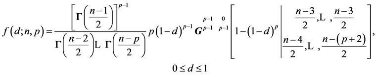
b) For the two-component case (p = 2), we have:
 (18)
(18)
2) For a non-fully independent two-component binormal system , for
, for :
:
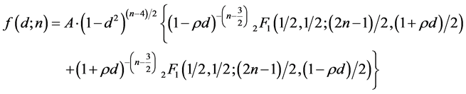 (19)
(19)
where
 and
and
 is Gauss hypergeometric function.
PROOF: a) For , the density of
 , as given by (17), is obtained
from (11) by a change of variable. Figure 4 gives
the density of the sample coefficient of inner dependence
, as given by (17), is obtained
from (11) by a change of variable. Figure 4 gives
the density of the sample coefficient of inner dependence , for n = 10 and p = 4.
Expression (18) is obtained from (15) by the change of variable . Again, the density of
d, as given by (19), can be derived from (16) by considering the same change of
variable. QED.
. Again, the density of
d, as given by (19), can be derived from (16) by considering the same change of
variable. QED.
Numerical computations give . Estimation of
 from
from
 now follows the same principles as
 from r.
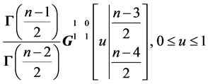
Figure 5 gives the density , as given by (19), for
n = 8, p = 2,
, as given by (19), for
n = 8, p = 2, .
.
6. Conclusion
In this article we have established an original expression for the density of the correlation matrix, with the sample variances as parameters, in the case of the multivariate normal population with non-identity population correlation matrix. We have, furthermore, established the expression of the distribution of the determinant of that random matrix in the case of identity population correlation matrix, and computed its value. Applications are
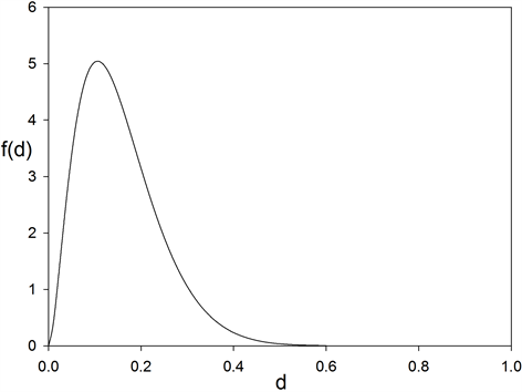
Figure 4. Density (17)
for sample coefficient of inner dependence
 (normal system with four components, n = 10, p = 4).
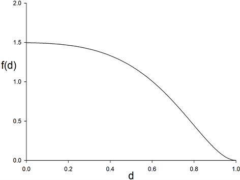
Figure 5. Density (19)
of sample measure of a binormal system dependence, .
.
made to the dependence among p components of a system. Also, expressions for the densities of a sample measure of a system inner dependence are established.
References
- Johnson, D. (1998) Applied Multivariate Methods for Data Analysis. Duxbury Press, Pacific Grove.
- Fisher, R.A. (1962) The Simultaneous Distribution of Correlation Coefficients. Sankhya, Series A, 24, 1-8.
- Pham-Gia, T. and Turkkan, N. (2011) Distributions of the Ratio: From Random Variables to Random Matrices. Open Journal of Statistics, 1, 93-104. http://dx.doi.org/10.4236/ojs.2011.12011
- Hotelling, H. (1953) New Light on the Correlation Coefficient and Its Transform. Journal of the Royal Statistical Society: Series B, 15, 193.
- Olkin, I. and Pratt, J.W. (1958) Unbiased Estimation of Certain Correlation Coefficients. Annals of Mathematical Statistics, 29, 201-211. http://dx.doi.org/10.1214/aoms/1177706717
- Joarder, A.H. and Ali, M.M. (1992) Distribution of the Correlation Matrix for a Class of Elliptical Models. Communications in Statistics—Theory and Methods, 21, 1953-1964. http://dx.doi.org/10.1080/03610929208830890
- Ali, M.M., Fraser, D.A.S. and Lee, Y.S. (1970) Distribution of the Correlation Matrix. Journal of Statistical Research, 4, 1-15.
- Fraser, D.A.S. (1968) The Structure of Inference. Wiley, New York.
- Schott, J. (1997) Matrix Analysis for Statisticians. Wiley, New York.
- Kollo, T. and Ruul, K. (2003) Approximations to the Distribution of the Sample Correlation Matrix. Journal of Multivariate Analysis, 85, 318-334. http://dx.doi.org/10.1016/S0047-259X(02)00037-4
- Farrell, R. (1985) Multivariate Calculation. Springer, New York. http://dx.doi.org/10.1007/978-1-4613-8528-8
- Gupta, A.K. and Nagar, D.K. (2000) Matrix Variate Distribution. Hall/CRC, Boca Raton.
- Mathai, A.M. and Haubold, P. (2008) Special Functions for Applied Scientists. Springer, New York. http://dx.doi.org/10.1007/978-0-387-75894-7
- Kshirsagar, A. (1972) Multivariate Analysis. Marcel Dekker, New York.
- Muirhead, R.J. (1982) Aspects of Multivariate Statistical Theory. Wiley, New York. http://dx.doi.org/10.1002/9780470316559
- Fisher, R.A. (1915) The Frequency Distribution of the Correlation Coefficient in Samples from an Indefinitely Large Population. Biometrika, 10, 507-521.
- Stuart, A. and Ord, K. (1987) Kendall’s Advanced Theory of Statistics, Vol. 1. 5th Edition, Oxford University Press, New York.
- Sawkins, D.T. (1944) Simple Regression and Correlation. Journal and Proceedings of the Royal Society of New South Wales, 77, 85-95.
- Pham-Gia, T., Turkkan, N. and Vovan, T. (2008) Statistical Discriminant Analysis Using the Maximum Function. Communications in Statistics-Simulation and Computation, 37, 320-336. http://dx.doi.org/10.1080/03610910701790475
- Nagar, D.K. and Castaneda, M.E. (2002) Distribution of Correlation Coefficient under Mixture Normal Model. Metrika, 55, 183-190. http://dx.doi.org/10.1007/s001840100139
- Gupta, A.K. and Nagar, D.K. (2004) Distribution of the Determinant of the Sample Correlation Matrix from a Mixture Normal Model. Random Operators and Stochastic Equations, 12, 193-199.
- Springer, M. (1984) The Algebra of Random Variables. Wiley, New York.
- Pham-Gia, T. (2008) Exact Distribution of the Generalized Wilks’s Statistic and Applications. Journal of Multivariate Analysis, 99, 1698-1716. http://dx.doi.org/10.1016/j.jmva.2008.01.021
- Pham-Gia, T. and Turkkan, N. (2002) Operations on the Generalized F-Variables, and Applications. Statistics, 36, 195-209. http://dx.doi.org/10.1080/02331880212855
- Pitman, E.J.G. (1937) Significance Tests Which May Be Applied to Samples from Any Population, II, the Correlation Coefficient Test. Supplement to the Journal of the Royal Statistical Society, 4, 225-232. http://dx.doi.org/10.2307/2983647
- Rencher, A.C. (1998) Multivariate Statistical Inference and Applications. Wiley, New York.
- Jogdev, K. (1982) Concepts of Dependence. In: Johnson, N. and Kotz, S., Eds., Encyclopedia of Statistics, Vol. 2, Wiley, New York, 324-334.
- Joe, H. (1997) Multivariate Models and Dependence Concepts. Chapman and Hall, London. http://dx.doi.org/10.1201/b13150
- Bertail, P., Doukhan, P. and Soulier, P. (2006) Dependence in Probability and Statistics. Springer Lecture Notes on Statistics 187, Springer, New York. http://dx.doi.org/10.1007/0-387-36062-X
- Drouet Mari, D. and Kotz, S. (2004) Correlation and Dependence. Imperial College Press, London.
- Lancaster, H.O. (1982) Measures and Indices of Dependence. In: Johnson, N. and Kotz, S., Eds., Encyclopedia of Statistics, Vol. 2, Wiley, New York, 334-339.
- Hoyland, A. and Rausand, M. (1994) System Reliability Theory. Wiley, New York.
- Bekker, A., Roux, J.J.J. and Pham-Gia, T. (2005) Operations on the Matrix Beta Type I and Applications. Unpublished Manuscript, University of Pretoria, Pretoria.