Open Journal of Statistics
Vol.3 No.6A(2013), Article ID:41361,5 pages DOI:10.4236/ojs.2013.36A002
Decompositions of Symmetry Using Generalized Linear Diagonals-Parameter Symmetry Model and Orthogonality of Test Statistic for Square Contingency Tables
1Department of Medical Innovation, Osaka University Hospital, Osaka, Japan
2Department of Information Sciences, Faculty of Science and Technology, Tokyo University of Science, Chiba, Japan
Email: yamamoto-k@hp-crc.med.osaka-u.ac.jp, o.motoki1211@gmail.com, tomizawa@is.noda.tus.ac.jp
Copyright © 2013 Kouji Yamamoto et al. This is an open access article distributed under the Creative Commons Attribution License, which permits unrestricted use, distribution, and reproduction in any medium, provided the original work is properly cited. In accordance of the Creative Commons Attribution License all Copyrights © 2013 are reserved for SCIRP and the owner of the intellectual property Kouji Yamamoto et al. All Copyright © 2013 are guarded by law and by SCIRP as a guardian.
Received October 10, 2013; revised November 10, 2013; accepted November 17, 2013
Keywords: Cumulative Probability; Global Symmetry; Linear Diagonals-Parameter Symmetry; Mean Equality; Ordinal Category; Orthogonal Test Statistic
ABSTRACT
For square contingency tables with ordered categories, the present paper gives several theorems that the symmetry model holds if and only if the generalized linear diagonals-parameter symmetry model for cell probabilities and for cumulative probabilities and the mean nonequality model of row and column variables hold. It also shows the orthogonality of statistic for testing goodness-of-fit of the symmetry model. An example is given.
1. Introduction
Consider an  square contingency table with the same row and column classifications. Let
  denote the probability that an observation will fall in the ith row and jth column of the table
  Bowker [1] considered the symmetry (S) model defined by
This model describes the structure of symmetry with respect to the cell probabilities  As a model which indicates the structure of asymmetry for
  Agresti [2] considered the linear diagonals-parameter symmetry (LDPS) model defined by
A special case of this model obtained by putting  is the S model. Yamamoto and Tomizawa [3] considered the generalized linear diagonals-parameter symmetry (LDPS(K)) model as follows; for a fixed
Especially the LDPS(0) model is equivalent to the LDPS model.
Let for 
 and
and 
The S model may be expressed as
Thus the S model also has the structure of symmetry with respect to the cumulative probabilities 
 Miyamoto et al. [4] considered the cumulative linear diagonals-parameter symmetry (CLDPS) model defined by
which indicates a structure of asymmetry for 
 The CLDPS model is different from the LDPS model. Yamamoto and Tomizawa [3] considered the generalized cumulative linear diagonals-parameter symmetry (CLDPS(K)) model as follows; for a fixed
Especially the CLDPS(0) model is equivalent to the CLDPS model.
Let  and
and  denote the row and column variables, respectively. We consider the mean equality (ME) model as
where  and
and 
 and
and 
Yamamoto et al. [5] gave Theorem 1. The S model holds if and only if both the LDPS and ME models hold.
Yamamoto and Tomizawa [6] gave Theorem 2. The S model holds if and only if both the CLDPS and ME models hold.
The present paper gives several decompositions of the S model using the LDPS(K) and CLDPS(K) models. It also proposes the mean nonequality model, and gives the orthogonal decomposition for testing goodness-of-fit of the S model. An example is given.
2. Decompositions of Symmetry Model
We shall give five kinds of decompositions of the S model using the LDPS(K) and CLDPS(K) models.
Theorem 3. For a fixed  the S model holds if and only if both the LDPS(K) and ME models hold.
Proof. If the S model holds, then both the LDPS(K) and ME models hold. Conversely, assuming that the LDPS(K) and ME models hold and then we shall show that the S model holds. The ME model may be expressed as
From the LDPS(K) model, we see
Therefore we obtain . Namely the S model holds. The proof is completed.
Theorem 4. For a fixed  the S model holds if and only if both the CLDPS(K) and ME models hold.
Considering the global symmetry (GS) model as
namely
we obtain Theorem 5. For a fixed  the S model holds if and only if both the LDPS(K) and GS models hold.
We shall omit the proofs of Theorems 4 and 5 because these are obtained in a similar manner to the proof of Theorem 3.
For a fixed  consider the mean nonequality (MNE(K)) model as follows:
which is
This model indicates that the difference between the means of  and
and  is
is  times higher than the difference between the global symmetric probabilities. When
  the MNE(0) model is identical to the ME model. We obtain Theorem 6. For a fixed
  the S model holds if and only if both the LDPS(K) and MNE(K) models hold.
Theorem 7. For a fixed  and for a fixed
  the S model holds if and only if both the LDPS(K) and MNE(L) models hold.
We shall omit the proofs of Theorems 6 and 7 because there are obtained in a similar manner to the proof of Theorem 3. Note that: 1) Theorem 6 is an extension of Theorem 1 because when  Theorem 6 is identical to Theorem 1; 2) Theorem 7 is an extension of Theorem 3 because when
  Theorem 7 is identical to Theorem 3; and 3) Theorem 7 is an extension of Theorem 6 because when
  Theorem 7 is identical to Theorem 6.
3. Test Statistic and Orthogonality
Let  denote the observed frequency in the ith row and jth column of the
  table with
  and let
  denote the corresponding expected frequency. Assume that
  has a multinomial distribution. The maximum likelihood estimates of expected frequencies
  under each model could be obtained, for example, using the Newton-Raphson method to the log-likelihood equations. Each model (say, model
 ) can be tested for goodness-of-fit by the likelihood ratio chi-squared statistic
  with the corresponding degrees of freedom, defined by
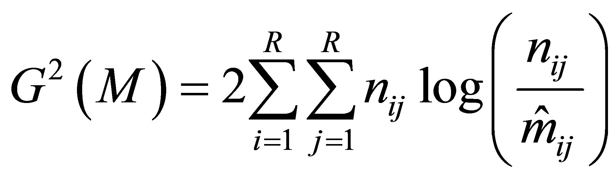
where  is the maximum likelihood estimate of
  under the model. The number of degrees of freedom for the S model is
  and that for each of the LDPS(K) and CLDPS(K) models is
  (being one less than that for the S model). That for each of ME, GS, and MNE(K) models is 1. Note that the number of degrees of freedom for the S model is equal to the sum of those for the decomposed models.
Lang and Agresti [7] and Lang [8] considered the simultaneous modeling of a model for the joint distribution and a model for the marginal distribution. Aitchison [9] discussed the asymptotic separability, which is equivalent to the orthogonality in Read [10] and the independence in Darroch and Silvey [11], of the test statistic for goodness-of-fit of two models (also see Tomizawa and Tahata [12], Tahata et al. [13], and Tahata and Tomizawa [14]). On the orthogonality of test statistic for models in Theorem 6, we obtain.
Theorem 8. For a fixed  test statistic
  is asymptotically equivalent to the sum of
  and
and 
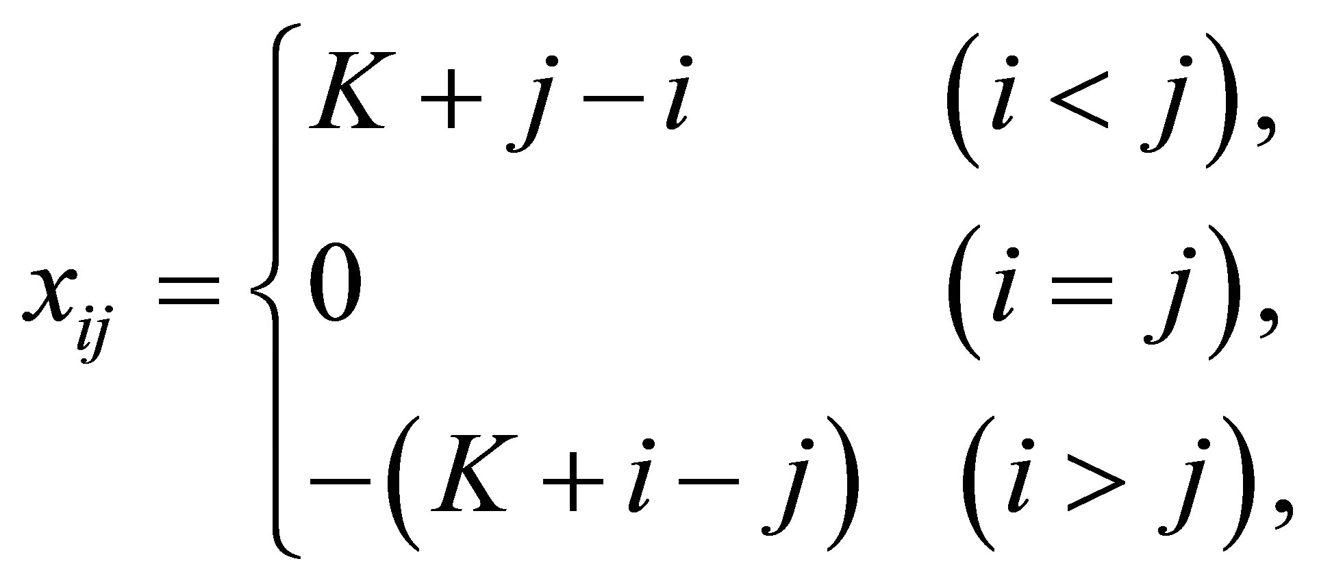
Proof. The LDPS(K) model may be expressed as
 (1)
(1)
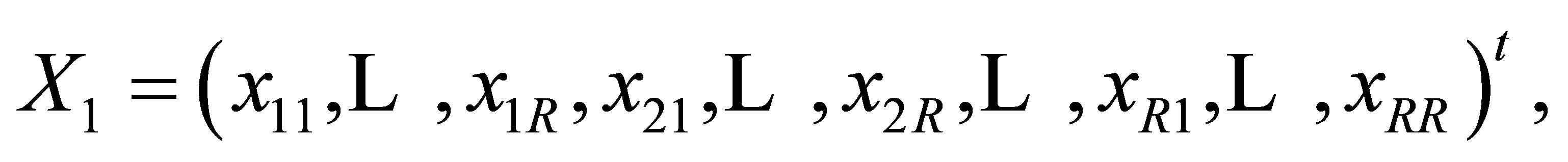
where  Let
Let
where “t” denotes the transpose, and
is the  vector. The LDPS(K) model is expressed as
where  is the
  matrix with
  and
and  is the
  vector with
where
and  is
is  matrix of 0 or 1 elements determined from (1). The matrix
  is full column rank which is
  In a similar manner to Haber [15], Lang and Agresti [7], and Tahata and Tomizawa [16], we denote the linear space spanned by columns of the matrix
  by
by  with the dimension
  Note that
  where
where  is the
  vector of 1 elements, and thus
  Let
Let  be an
be an  where
where  full column rank matrix such that the linear space
  is the orthogonal component of the space
  Thus,
Thus,  where
where  is the
  zero matrix. Therefore, the LDPS(K) model is expressed as
where  is the
  zero matrix, and
The MNE(K) model may be expressed as

where 
Note that  From Theorem 6, the S model may be expressed as
where 

Note that  are the numbers of degrees of freedom for testing goodness-of-fit of the LDPS(K), MNE(K) and S models, respectively.
Let  denote the
  matrix of partial derivatives of
  with respect to
  i.e.,
i.e.,  Let
Let  where
where  denotes a diagonal matrix with ith component of
  as ith diagonal component. We see that
because  and that
Thus we obtain
Therefore we obtain  where
where
From the asymptotic equivalence of the Wald statistic and the likelihood ratio statistic (Rao [17], Darroch and Silvey [11], Aitchison [9]), we obtain Theorem 8. The proof is completed.
4. Analysis of Data
Table 1 taken directly from Agresti [18, p. 232] summarizes responses to the questions “How successful is the government in (1) providing health care for the sick? (2) Protecting the environment?”.
Table 2 gives the values of the likelihood ratio test statistic  for models applied to these data. The S model does not fit these data so well. Also, each of the ME (i.e., MNE(0)), MNE(K)
  and the GS models does not fit these data so well. However each of the LDPS(K) models
  and the CLDPS(K) models
  fit these data very well. Using Theorems 3 through 7 (including Theorems 1 and 2), we shall consider the reason why the S model fits these data poorly. For the structure of cell probabilities
  we see from Theorems 3, 5, 6 and 7 that the poor fit of the S model is caused by the influence of the lack of structure of the ME model (the GS model or the MNE(K) model
 ) rather than the LDPS(K) model
  For the structure of cumulative probabilities
 we see from Theorem 4 that the poor fit of the S model is caused by the influence of the lack of structure of the ME model rather than the CLDPS(K) model
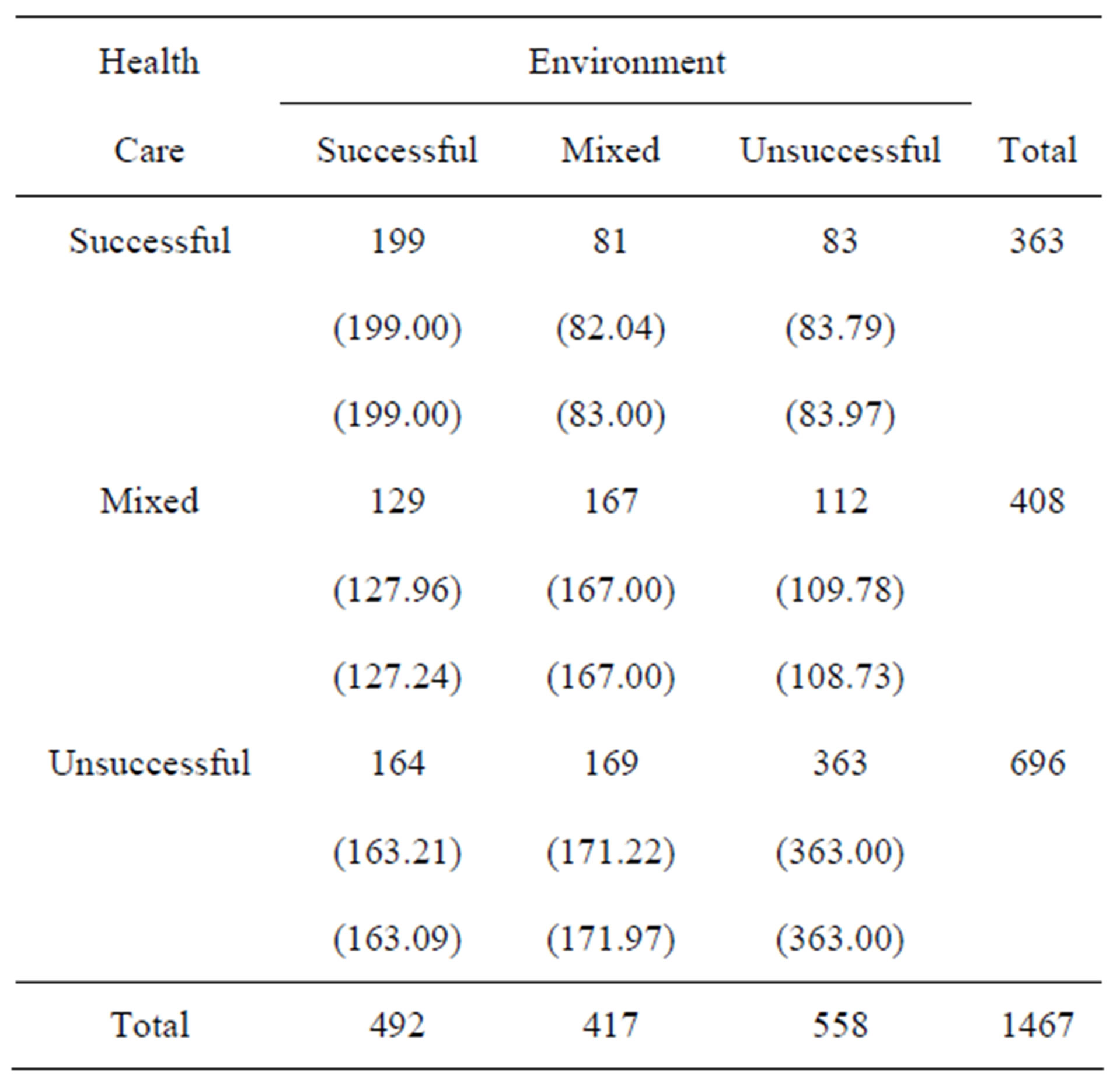
Table 1. Data on success of US government in providing health care and protecting the environment; from Agresti [18, p. 232]. (Upper and lower parenthesized values are maximum likelihood estimates of expected frequencies under the LDPS(1) and CLDPS(4) models, respectively.)
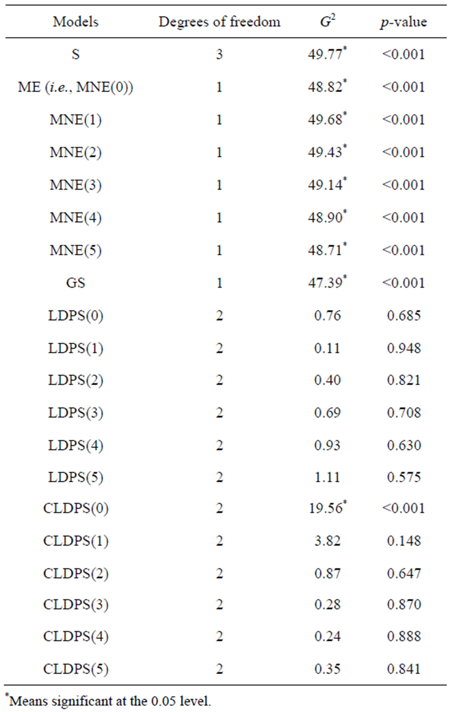
Table 2. Values of likelihood ratio chi-squared statistic G2 for models applied to the data in Table 1.
5. Concluding Remarks
We have given the new five kinds of decompositions of the S model. Theorems 3 and 4 are extensions of Theorems 1 and 2, respectively. Theorem 5 is another decomposition of the S model. Theorem 6 is another extension of Theorem 1, and Theorem 7 is an extension of Theorem 3. These theorems may be useful for seeing in more details the reason for the poor fit when the S model fits the data poorly.
From the orthogonality of test statistic given by Theorem 8, we point out that for instance, the likelihood ratio chi-squared statistic for testing goodness-of-fit of the S model assuming that the LDPS(K) model holds true is  and this is asymptotically equivalent to the likelihood ratio chi-squared statistic for testing goodness-of-fit of the MNE(K) model, i.e.,
  We see that for the data in Table 1 the value of
  is very close to the sum of the values of
  and
and  (see Table 2). The orthogonal decomposition of the S model into the LDPS(K) and MNE(K) models would guarantee that (1) if both the LDPS(K) and MNE(K) models are accepted (e.g., at the 0.05 significance level) with high probability, then the S model would be accepted, and (2) it would be impossible to arise such an incompatible situation that both the LDPS(K) and MNE(K) models are accepted with high probability but the S model is rejected with high probability. Therefore, in particular Theorems 6 and 8 would be useful for analyzing the data.
REFERENCES
- A. H. Bowker, “A Test for Symmetry in Contingency Tables,” Journal of the American Statistical Association, Vol. 43, No. 244, 1948, pp. 572-574. http://dx.doi.org/10.1080/01621459.1948.10483284
- A. Agresti, “A Simple Diagonals-Parameter Symmetry and Quasi-Symmetry Model,” Statistics and Probability Letters, Vol. 1, No. 6, 1983, pp. 313-316. http://dx.doi.org/10.1016/0167-7152(83)90051-2
- K. Yamamoto and S. Tomizawa, “Statistical Analysis of Case-Control Data of Endometrial Cancer Based on New Asymmetry Models,” Journal of Biometrics and Biostatistics, Vol. 3, No. 5, 2012, pp. 1-4. http://dx.doi.org/10.4172/2155-6180.1000147
- N. Miyamoto, W. Ohtsuka and S. Tomizawa, “Linear Diagonals-Parameter Symmetry and Quasi-Symmetry Models for Cumulative Probabilities in Square Contingency Tables with Ordered Categories,” Biometrical Journal, Vol. 46, No. 6, 2004, pp. 664-674. http://dx.doi.org/10.1002/bimj.200410066
- H. Yamamoto, T. Iwashita and S. Tomizawa, “Decomposition of Symmetry into Ordinal Quasi-Symmetry and Marginal Equimoment for Multi-way Tables,” Austrian Journal of Statistics, Vol. 36, No. 4, 2007, pp. 291-306.
- K. Yamamoto and S. Tomizawa, “Analysis of Unaided Vision Data Using New Decomposition of Symmetry,” American Medical Journal, Vol. 3, No. 1, 2012, pp. 37- 42. http://dx.doi.org/10.3844/amjsp.2012.37.42
- J. B. Lang and A. Agresti, “Simultaneously Modeling Joint and Marginal Distributions of Multivariate Categorical Responses,” Journal of the American Statistical Association, Vol. 89, No. 426, 1994, pp. 625-632. http://dx.doi.org/10.1080/01621459.1994.10476787
- J. B. Lang, “On the Partitioning of Goodness-of-Fit Statistics for Multivariate Categorical Response Models,” Journal of the American Statistical Association, Vol. 91, No. 435, 1996, pp. 1017-1023. http://dx.doi.org/10.1080/01621459.1996.10476972
- J. Aitchison, “Large-Sample Restricted Parametric Tests,” Journal of the Royal Statistical Society: Series B, Vol. 24, No. 1, 1962, pp. 234-250.
- C. B. Read, “Partitioning Chi-Square in Contingency Tables: A Teaching Approach,” Communications in Statistics-Theory and Methods, Vol. 6, No. 6, 1977, pp. 553- 562. http://dx.doi.org/10.1080/03610927708827513
- J. N. Darroch and S. D. Silvey, “On Testing More than One Hypothesis,” Annals of Mathematical Statistics, Vol. 34, No. 2, 1963, pp. 555-567. http://dx.doi.org/10.1214/aoms/1177704168
- S. Tomizawa and K. Tahata, “The Analysis of Symmetry and Asymmetry: Orthogonality of Decomposition of Symmetry into Quasi-Symmetry and Marginal Symmetry for Multi-Way Tables,” Journal de la Société Francaise de Statistique, Vol. 148, No. 3, 2007, pp. 3-36.
- K. Tahata, H. Yamamoto and S. Tomizawa, “Orthogonality of Decompositions of Symmetry into Extended Symmetry and Marginal Equimoment for Multi-Way Tables with Ordered Categories,” Austrian Journal of Statistics, Vol. 37, No. 2, 2008, pp. 185-194.
- K. Tahata and S. Tomizawa, “Orthogonal Decomposition of Point-Symmetry for Multiway Tables,” Advances in Statistical Analysis, Vol. 92, No. 3, 2008, pp. 255-269. http://dx.doi.org/10.1007/s10182-008-0070-5
- M. Haber, “Maximum Likelihood Methods for Linear and Log-Linear Models in Categorical Data,” Computational Statistics and Data Analysis, Vol. 3, No. 1, 1985, pp. 1- 10. http://dx.doi.org/10.1016/0167-9473(85)90053-2
- K. Tahata and S. Tomizawa, “Double Linear DiagonalsParameter Symmetry and Decomposition of Double Symmetry for Square Tables,” Statistical Methods and Applications, Vol. 19, No. 3, 2010, pp. 307-318. http://dx.doi.org/10.1007/s10260-009-0127-y
- C. R. Rao, “Linear Statistical Inference and its Applications,” 2nd Edition, John Wiley, New York, 1973. http://dx.doi.org/10.1002/9780470316436
- A. Agresti, “Analysis of Ordinal Categorical Data,” 2nd Edition, John Wiley, Hoboken, 2010. http://dx.doi.org/10.1002/9780470594001