Open Journal of Statistics
Vol. 2 No. 1 (2012) , Article ID: 17139 , 9 pages DOI:10.4236/ojs.2012.21002
Finite Mixture of Heteroscedastic Single-Index Models
Department of Mathematics and Statistics, Auburn University, Auburn, USA
Email: zengpen@auburn.edu
Received May 22, 2011; revised June 28, 2011; accepted July 8, 2011
Keywords: EM Algorithm; Finite Mixture Model; Heterogeneity; Heteroscedasticity; Local Linear Smoothing; Single-Index Model
ABSTRACT
In many applications a heterogeneous population consists of several subpopulations. When each subpopulation can be adequately modeled by a heteroscedastic single-index model, the whole population is characterized by a finite mixture of heteroscedastic single-index models. In this article, we propose an estimation algorithm for fitting this model, and discuss the implementation in detail. Simulation studies are used to demonstrate the performance of the algorithm, and a real example is used to illustrate the application of the model.
1. Introduction
When it is difficult to specify a parametric model due to the lack of enough prior knowledge, researchers often consider a semi-parametric model as alternative, where a nonparametric component is added to encompass a wide range of models and ensure more flexibility. Single-index model is such a typical example. It assumes that a univariate response  depends on a vector of predictors
 via its linear combination,
 (1)
(1)
where β is a vector of unit length,  is an unknown univariate function, and ε is a random error such that
  and
and . Model (1) generalizes the ordinary linear regression by leaving
  unspecified. Meanwhile, it still maintains enough interpretability, for β can be interpreted similarly as the coefficients in a linear regression model. See [1-3] and references therein for more discussions.
The single-index model (1) assumes a homoscedastic variance, which may be limited in some applications. A natural generalization is to consider a heteroscedastic single-index model (hetero-SIM), which assumes
 (2)
(2)
where  and
and  are two unknown univariate functions and ε is a random error such that
  and
and . The model (1) is thus referred to as a homo-SIM, which is a special case of (2) when
 . [4] proposed an estimation algorithm to (2) when
  and studied its theoretical property in detail.
In a homo-or hetero-SIM, because β can be estimated at root-n rate of convergence as showed in the aforementioned articles, the asymptotic properties of the estimates of  and
and  are similar to those in univariate nonparametric problems. Thus homoor hetero-SIM are free of curse of dimensionality in high dimensional data analysis. They also provide a convenient way to visualize data by plotting Y against βTX.
In many applications the population under study is not homogenous and a single-index model is not flexible enough to characterize its complex structure. The heterogeneity may result from various reasons, such as the omission of important categorical variables, the ignorance of hidden structural changes, and unknown segmentation in the population. In these cases, the heterogenous population consists of several subpopulations. We may assume that how the response Y depends on predictor X varies for each subpopulation, and each subpopulation can be adequately modeled by  , where
  c and c is the number of subpopulations. Therefore, the whole population is characterized by a mixture of regressions. This model is referred to as a finite mixture of heteroSIMs.
There are some similar models studied by researchers in a variety of areas, which include switching regression [5] in economics, clusterwise linear regression [6] in marketing, mixture-of-experts model [7] in machine learning, and mixture of Poisson regression models [8] in biology. However, in these models  is either linear or known and
  is usually a constant. As a contrast, finite mixture of hetero-SIMs provides more flexibility in modeling by allowing
  and
and  to be unknown.
The difficulty in model fitting lies in three aspects. First, we do not know which subpopulation each observation comes from; second, the functions  and
and  are unknown; third, the response depends on βk through a nonlinear relation. In this article, we embed finite mixture of hetero-SIMs into the framework of finite mixture models [9], and apply EM algorithm [10,11] to calculate the estimates. Notice that a finite mixture model is usually intended to model the joint distribution of all variables. But finite mixture of hetero-SIMs only concentrates on the conditional distribution of
 , and the predictor X is treated as fixed constant. The second difficulty is tackled by applying local linear smoothing [12] to estimate
  and
and . The third difficulty is solved by employing a variant of Newton-Raphson algorithm.
One alternative approach to fit the mixture of regressions is to proceed in two steps: first identify subpopulations by a clustering method, and then fit a single-index model for each subpopulation. We argue that our proposed algorithm is preferable to this two-step procedure. Firstly, if the clustering analysis is conducted based only on predictor X, it essentially classifies observations according to the distribution of X. The obtained results of clustering may not be relevant to the truth, because the true subpopulations are defined with respect to the conditional distribution of . Secondly, if the clustering analysis is conducted based on both response Y and predictor X, any assumptions on the joint distribution of Y and X implicitly impose some restrictions on how Y depends X. In either case, we have to specify a distribution for a vector
 , whose dimension may be high. Besides, the predictors usually contain both continuous and categorical variables, which introduces extra difficulty in clustering analysis. But for finite mixture of hetero-SIMs, we only need to specify the distribution of the univariate random errors.
The remaining part of this article is organized as follows. Section 2 discusses an algorithm for estimating a hetero-SIM. Section 3 focuses on how to estimate finite mixture of hetero-SIMs. More detailed discussions on implementation are contained in Section 4. Section 5 demonstrates the performance of the proposed algorithm by some simulation studies. A real example is used to illustrate the application of finite mixture of hetero-SIMs. Section 6 ends this article with some concluding remarks.
2. Heteroscedastic Single-Index Models
This section discusses the estimation algorithm for a hetero-SIM (2). We only focus on the case where ε is normally distributed; see Section 6 for discussions on other distributions. It can be verified that the conditional mean  and the conditional variance
 . Thus the model (2) can be equivalently represented as
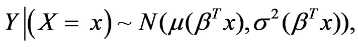 (3)
(3)
where  denotes a normal distribution with mean μ and variance σ2.
Suppose that the observations are independently sampled from model (3), and a nonnegative weight wi is associated with each observation
 . We need to estimate a d-dimensional parameter β and two unknown functions μ and σ2. A natural approach is to find the estimates of β, μ, and σ2 by maximizing the weighted sum of log-densities,
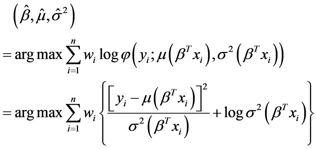
where  is the density function of
 . This objective function is different from the commonlyused weighted squared loss function in that the heteroscedasticity is incorporated. Thus this estimate of β is expected to have better performance than that when the heteroscedasticity is ignored, which is demonstrated using simulation studies in Section 4.
It is unrealistic to solve the optimization problem directly. A more computationally feasible approach is to treat β and  as two groups of parameters, and then iteratively update the values of the parameters in one group when the other group of parameters remains fixed. When μ and σ2 are known, calculating β is a finite-dimensional nonlinear minimization problem, while when β is given, the estimation of μ and σ2 are univariate nonparametric problems. We derive the two components in detail in the following.
When μ and σ2 are given, we calculate β by
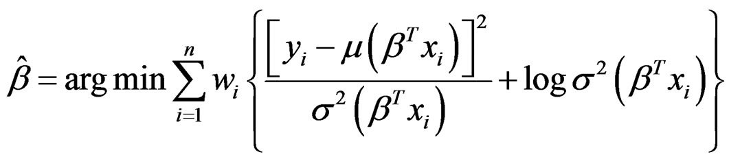
There is no closed form for the solution of β to this nonlinear optimization problem. A popular way of calculating a numerical solution is to apply Newton-Raphson algorithm. Denote the objective function as  and it can be derived that
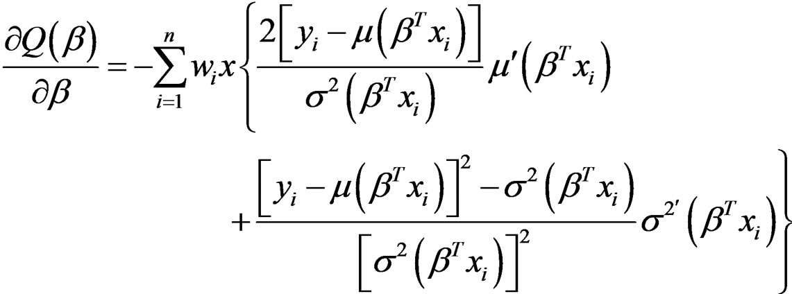
where  and
and  are the first derivatives of μ and σ2, respectively. The second derivative (Hessian matrix) of
  has a complicated expression, which involves the second derivatives of μ and σ2. To simplify the calculation, we consider the expectation of the Hessian matrix of
  instead. Because

the expectation of the Hessian matrix can be written as

There is no need to calculate the second derivatives of μ and σ2 in the above expression. Notice that the similar idea is used in fitting a generalized linear model. The formula for updating the estimate of β is thus
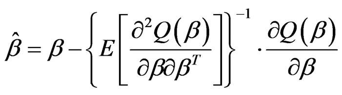 (4)
(4)
Because μ and σ2 are unknown, they are substituted by the corresponding estimates.
Now let us discuss how to estimate μ and σ2 when β is given. In this case, we need to find the estimates of μ and σ2 by
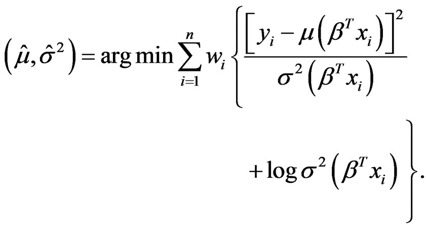
Because β is known, it is essentially a univariate nonparametric problem to estimate functions μ and σ2 from the following model,
where , the weight associated with
  is wi, and εi are iid
 . There are many literatures on this univariate heteroscedastic regression problem; see [13-15] and references therein for more discussions. One possible approach is to estimate μ and σ2 using local likelihood method following the discussion in Section 4.9 of [12]. However, it is computationally intractable. [15] proposed an algorithm that is much computationally easier and meanwhile preserves the efficiency of the estimates.
[15] recommended to first estimate the mean function by local linear smoothing [12]. Therefore,  , where
where K1 is a kernel function and h1 is a bandwidth. Because , the variance function can be treated as a mean function and can also be estimated via local linear smoothing. Hence, calculate the squared residuals
  and estimate
 , where
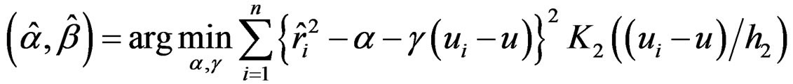
where K2 is another kernel function and h2 is a bandwidth, which may not be the same as K1 and h1 used for estimating the mean function μ. The first derivatives of μ and σ2 are needed in evaluating (4). They are estimated by  and
and ,respectively.
In order to fit a hetero-SIM, we assemble the two components discussed above together. The initial value of β, β(0) can be chosen as the least squares estimate of a linear regression model. In each iteration step, we first estimate  and
and  with given
 , then calculate β(m) using equation (4), and last evaluate
 . The iterations proceed until the difference between the values of
  in two successive iterations is smaller than a pre-specified tolerance value. An alternative way to check convergence is to compare the values of β in two successive iterations.
3. Finite Mixture of Hetero-SIMs
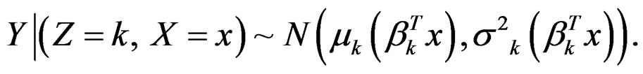
A finite mixture of hetero-SIMs can be used to model a heterogeneous population. Suppose that the observations  are independently sampled from a population consisting of c normal subpopulations,

where βk’s are vectors of unit length, πk’s are positive values such that  and
and , and μk’s and σ2k’s are unknown univariate functions. For the purpose of identifiability, we assume that
  and
and , if
, if ’. It is convenient to represent the above finite mixture model in terms of a hierarchical model by introducing an unobserved variable Z to indicate which subpopulation an observation is sampled from,

The marginal distribution of Y (averaging out Z, but still conditionally on X) is exactly the distribution of Y in the finite mixture of hetero-SIMs. Although the distribution of Y depends on X via several different linear combinations, within each subpopulation, the response is adequately modeled by a hetero-SIM.
The conditional mean of  has the following expression
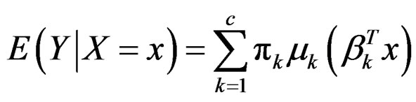
which resembles projection pursuit regression [16]. However, there are two major differences between projection pursuit regression and finite mixture of heteroSIMs. Firstly, the latter also models the conditional variance of Y, while the former does not. Secondly, the latter assumes an underlying heterogeneous structure, while the former only focuses on the prediction of the response. Hence the latter model can be used for clustering analysis, while the former cannot. As we can see latter, the fitting of finite mixture of hetero-SIMs utilizes a variant of EM algorithm, which is quite different from the fitting of projection pursuit regression.
For convenience, denote , where
 ,
,  ,
,  and
and . Notice that π and β are finite-dimensional parameters, while μ and σ2 are unknown functions. The log-likelihood function is
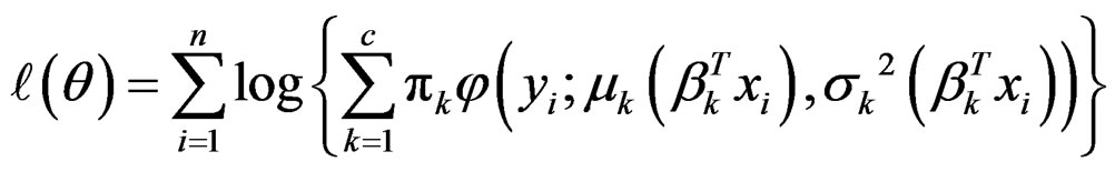
An appropriate estimate of θ is the MLE that maximizes .
.
It is difficult to estimate the unknown parameter θ by maximizing  directly. The popular approach to fitting a finite mixture model is to apply EM algorithm [9-11]. The EM algorithm consists of an expectation step (E-step) and a maximization step (M-step). We derive the detail in the following.
By including the unobserved variable Z, the “complete” data are . The joint density function of Y and Z (conditionally on X) is
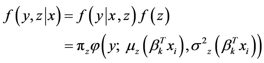
where  because Z is independent of X. Therefore, the complete loglikelihood function is
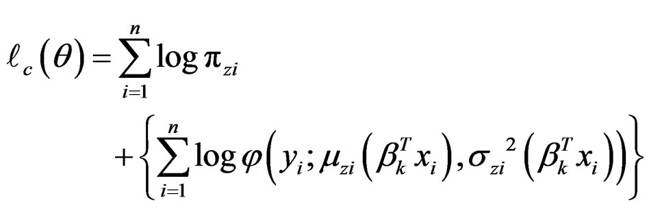
In the E-step, the (conditional) expectation of the complete log-likelihood function under the current value of θ* is calculated. The expectation of  is
is

where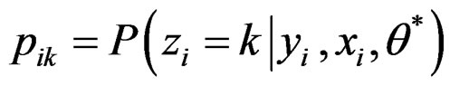 is the conditional probability that the ith observation is sampled from the kth subpopulation,
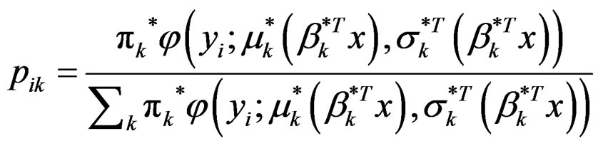 (5)
(5)
In the M-step, an updated value of θ is calculated by maximizing  obtained in the E-step. Some calculations yield the updated value of θ,
 (6)
(6)
and
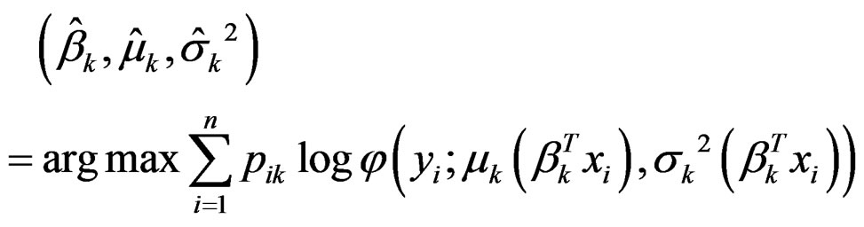 (7)
(7)
The estimates ,
,  ,
,  are calculated from fitting a hetero-SIM as discussed in Section 2. Notice that the associated weights are pik.
The initial values of pik and βk are needed to start iterations. In each iteration step, first calculate using (6), then estimate βk, μk, σk2 in (7), and last calculate pik by (5). The value of
  can be used to check if the algorithm converges or not. More detailed discussions of implementation are contained in the next section.
4. Implementation
In the previous two sections, the algorithm for fitting a finite mixture of hetero-SIMs has been derived. In this section, we first list the steps to fit the model, and then explain each step in detail.
When the number of subpopulations, c, is known, fit a finite mixture of hetero-SIMs following the steps below.
1) Initialization:
a) choose initial values of ,
, ;
;
b) calculate  for
for ;
; .
.
2) Iteration: for given βk(m) and pik(m)a) calculate  using (6);
b) calculate  and σ2k(m+1) and their derivatives;
c) calculate  using (4);
d) calculate  using (5);
e) calculate .
.
3) Check convergence: if , where ℓ is a pre-specified tolerance value, stop and output
 ; otherwise go back to Step 2) for another iteration.
A good choice of initial values usually leads to fast convergence. We recommend to set  as the estimated indexes from projection pursuit regression, or as the basis estimated by a sufficient dimension reduction method. Notice that sufficient dimension reduction can be used to estimate the linear space spanned by
  without specifying a parametric model; see [17-19] and references therein for more discussions. Because of the risk that the iterations stop at local maxima, it is always wise to start with different initial values and report the best results. When the initial value
  is given, we fit a simple linear regression of yi on
  xi and calculate residuals rik. The initial value of pik is cal culated as
 .
.
In the iteration step, local linear smoothing needed by Step 2b) is the most computationally intensive part. To speed up calculation, the linear binning algorithm [12] is used to implement local linear smoothing. The value of bandwidth usually influences the performance of estimating μk and σk2. There are many literatures on how to choose an optimal bandwidth automatically and adaptively from data; see [12,20] and reference therein. When a bandwidth selector is determined, we can select a bandwidth automatically whenever it is needed. The plug-in bandwidth selector [20] is used in the simulation studies. Although achieving good performance, it is computationally intensive, and may not be necessary. Simulation studies show that the performance of estimating βk is less sensitive to bandwidth than that of estimating functions. Thus it is possible to first estimate βk using a fixed rough bandwidth throughout the iteration steps and then fit μk and σk2 using a more refined bandwidth after the algorithm converges. Specifically, we recommend the rule-of-thumb bandwidth [21], which is simple and works well in simulation studies.
Another concern in Step 2b) is that some misclassified observations or outliers may severely deteriorate the performance of the estimates, because the estimated nonparametric functions are forced to adjust to the false pattern induced by them. Noticing that misclassified observations or outliers usually have extremely small densities, we recommend removing 5% of observations with the smallest densities when fitting μk and σk2. Our experience shows that the performance becomes more robust after trimming.
In Step 2c), the estimates of mean and variance functions, as well as their first derivatives, are needed to update βk. Because the performance of the estimates of the first derivatives may exhibit erratic behaviors near the boundary, we recommend removing 1% of observations near both sides of the boundary. Notice that the boundary means the smallest or the largest values of , and thus they are determined in each iteration.
The number of subpopulations, c, is usually unknown in practice, and needs to be determined from data. A subjective method is to choose c by examining the plots of yi against  for
for . If c is underestimated, some plots must demonstrate a clear lack-of-fitting. When c is overestimated, some subpopulations are further divided, in which case some βk are very close to each other. In fact, the dimension of the linear space spanned by
  chosen by sufficient dimension reduction methods may serve as an estimate of c, which is usually determined by a series of hypothesis testing; see [17,18] and reference therein.
5. Examples
Example 1. Consider the following hetero-SIM

where ,
,  and
and . The elements of X are independently sampled from uniform (−2, 2). We randomly generate 300 samples each of size n = 400 from this artificial model. The algorithm derived in Section 2 is used for model fitting. In this example, we only demonstrate the performance of estimating β, and omit the discussions on mean and variance functions, because after β is estimated, it becomes a univariate problem to estimate both functions, which have already been elaborated in [15].
The performance of an estimate is measured by
 , the angle (in degree) between this estimate and the true value β. It is clear that
  varies from 0˚ to 90˚, and the smaller the better. We first fit the 300 samples separately with different fixed bandwidth h = 0.2, 0.3, 0.4, 0.5, 0.6 and calculate
  for each estimate. Additionally, we fit the samples with the plug-in bandwidth [20] that is calculated from data in each iteration step whenever it is needed, which is referred to as h = “auto”. The left plot in Figure 1 demonstrates the influence of bandwidth using side-by-side boxplots. It is observed that the influence of bandwidth to the estimation of β is not severe. A wide range of bandwidth yields similar performance. It is unnecessary to choose an optimal bandwidth whenever it is needed.
In order to demonstrate the efficiency in estimating β gained by considering the heteroscedastic variance, we fit the 300 samples by assuming a homoscedastic variance. The performance of estimating β is displayed using side-by-side boxplots in the right plot of Figure 1. The influence of bandwidth is not severe. The performance is worse than that from hetero-SIM as expected.
The proposed algorithm achieves high efficiency in estimating β in that the estimate of β cannot be better even if the mean and variance functions are known. When the mean and variance functions are known, the only unknown parameter is β, which can be estimated by repeatedly applying (4). Using this method we fit the 300 samples and calculate . We compare the performance of estimating β in this case with that from a hetero-SIM with h = “auto” in the left plot of Figure 2. The straight line indicates where the two methods yield the same performance. It suggests that there is no much difference.
In practice, it is usually enough to use a rough bandwidth to estimate β. We first calculate the rule-of-thumb bandwidth for each component of X, and use their average as the bandwidth for fitting a hetero-SIM, which is referred to as h = “rot”. The performance of estimating β in this case is compared with that when the mean and variance functions are known in the right plot of Figure 2. It is observed that there is no much difference between these two methods. Therefore, it is enough to use a rough bandwidth in the estimation of β.
Example 2. Consider a finite mixture of two heteroSIMs.
 , with probability 0.6,
 , with probability 0.4where
 ,
,
 and
and ,
,


and . The elements of X are independently sampled from uniform(−2, 2). We randomly generate 300 samples each of size
 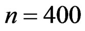 from this model.
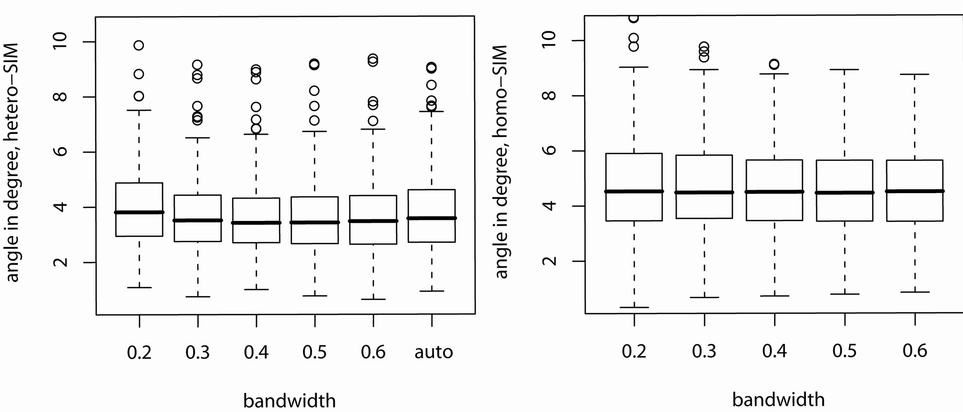
Figure 1. The side-by-side boxplots compare the performance of estimating β with different bandwidths, where β is estimated using hetero-SIM in the left plot and β is estimated using homo-SIM in the right plot.
Figure 2. The two plots compare the performance of estimating β when mean and variance functions are known with that when they are unknown. In the left plot, the plug-in bandwidth is used, while in the right plot, the rule-of-thumb bandwidth is used.
We first examine the influence of bandwidth on the estimating of βk. The samples are fitted using the algorithm discussed in Section 3 with bandwidth h = 0.2, 0.3, 0.4, 0.5, 0.6, “auto”, and “rot”; see Example 1 for the meaning of “auto” and “rot”. The results are summarized in Figure 3, where the lines marked by 1, 2, 3, 4, 5 correspond to the 5%, 25%, 50%, 75%, and 95% percentiles. The performances of estimating β1 and β2 share a similar pattern. For most samples (at least 75% of samples), the performance is not severely affected by bandwidth. But when the bandwidth is too large or too small, the probability that the algorithm stops at local maxima increases. It is the reason why the algorithm sometimes fails to estimate parameters consistently. However, this probability can be greatly reduced if we start the iterations with different initial values and choose the best result.
Figure 4 shows the scatter plot of yi against the projections of β1Txi and β2Txi for one typical sample. In both plots the two subpopulations are distinguished by dots (or circles) and triangles. The solid lines indicate the estimated mean function  and the two dash lines are
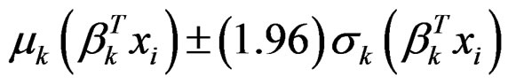 . Although the two subpopulations are mixed together, the algorithm successfully estimates μk and σk accurately. We can cluster the observations according to the values of pik. One observation is claimed to be in the first subpopulation if
 , and in the second subpopulation otherwise. In Figure 4, the dots and filled triangles indicate correctly classified observations, and circles and unfilled triangles indicate misclassified observations. The majority of observations are correctly classified. In fact most misclassifications occur when the observations are close to where the two response surfaces intersect.
The performance of estimating μk and σk can be measured by mean absolute deviation error,
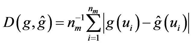
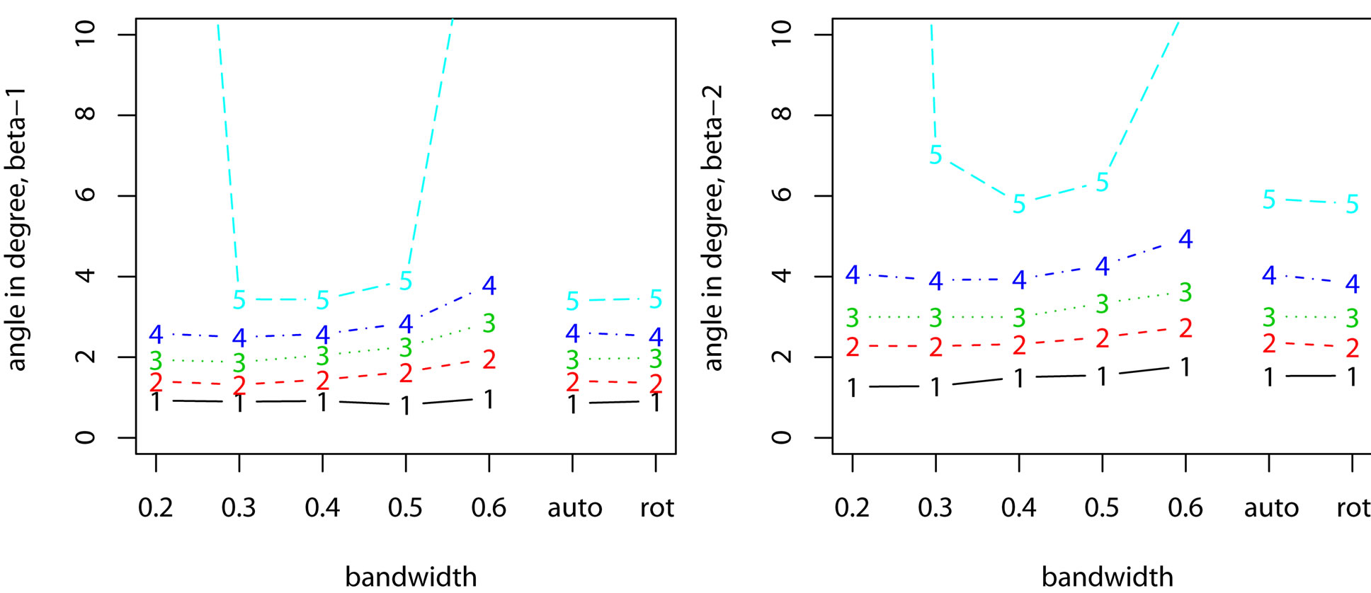
Figure 3. The plots compare the performance of estimating βk with different bandwidths. The lines marked by 1, 2, 3, 4, 5 correspond to 5%, 25%, 50%, 75%, 95% percentiles, respectively.

Figure 4. The scatter plots of yi against the projection of  for a typical example. The solid lines correspond to
 , and the dash lines correspond to are
 .
.
where g = μk or σk, and  are nm = 101 equally-spaced points in interval (−2.5, 2.5). The results are summarized in Figure 5, where the samples are fitted with the rule-of-thumb bandwidth. The performance shows the algorithm accurately estimate μk and σk. We also calculate the misclassification rate as the average proportion of the misclassified observations. The first quartile, median, and the third quartile are 0.048, 0.055, and 0.065, respectively. As we can observe from Figure 4, most misclassifications occur when the observations are close to where the two response surfaces intersect. Because these observations fall on both response surfaces, it is unlikely to correctly classify them according to the conditional distribution of
 . Other information or assumptions are needed to handle these observations.
Example 3. We consider 1985 Automobile Data, which is available at the UCI Machine Learning Repository. This dataset contains many different attributes on 205 cars. The objective of our analysis is to explain how the price of a car depends on its features. After removing cases with missing values, there are 195 observations left. Because some variables are highly linearly correlated with other variables, we remove them if the correlation coefficients exceed ±0.8. Therefore, in the following analysis the response is the logarithm of price  and the predictors are wheel base
 , height
 , curb weight
 , bore
 , stroke
 , compression ratio
 , horsepower
 , and peak rpm
 . In the beginning of analysis, each predictor is standardized by subtracting its mean and then being divided by its standard deviation.
The rule-of-thumb bandwidth is h = 0.31. We fit a model with two subpopulations. The proportions for the two subpopulations are  and
and , respectively. The estimates of βk are listed in Table 1. The angle between β1 and β2 is about 40˚.
The curb weight  and horsepower
  are the two most important features in determining the price of a car. The horsepower characterizes the performance of a car, while the engine size reflects the overall size of a car because it is highly positively linearly correlated with the length and width. The first subpopulation weights performance more than the overall size, and the second subpopulation is just the opposite.
6. Conclusions and Discussions
In this article, we propose a finite mixture of heteroSIMs, and discuss its estimation algorithm in detail. Although we assume that the random errors are normally distributed, it is not an essential assumption. The algorithm can be easily generalized to exponential family of distributions to allow binary or Poisson responses.
The finite mixture of hetero-SIMs is a semi-parametric model, where πk and βk are parametric components and μk and σk are nonparametric components. It is conjectured that the estimates of βk can achieve root-n rate of convergence as in a single-index model. The rigorous theoretical deviation needs much more efforts and will be reported elsewhere later.

Figure 5. The plots demonstrate the performance of estimating μk and . The lines marked by 1, 2, 3, 4, 5 correspond to 5%, 25%, 50%, 75%, 95% percentiles, respectively.

Table 1. Estimates of βk for automobile data.
The selection of number of subpopulations c is not fully explored in this article. We simply recommend choosing c according to sufficient dimension reduction. Popular methods for determining c in a finite mixture model are the information criteria such as AIC and BIC; see [9] for more discussions. Because of the present of nonparametric components, AIC and BIC are not directly applicable for finite mixture of hetero-SIMs.
There are also many other potential applications of the proposed model. For example, when testing the goodness-of-fit for a hetero-SIM or a finite mixture of linear regressions, it is appropriate to choose finite mixture of hetero-SIMs as the alternative. We will explore along these interesting directions in the future.
REFERENCES
- W. Härdle and T. M. Stoker, “Investigating Smooth Multiple Regression by the Method of Average Derivatives,” Journal of the American Statistical Association, Vol. 84, No. 408, 1989, pp. 986-995. doi:10.2307/2290074
- W. K. Newey and T. M. Stoker, “Efficiency of Weighted Average Derivative Estimators and Index Models,” Econometrica, Vol. 61, No. 5, 1993, pp. 1199-1223. doi:10.2307/2951498
- Y. Xia, “Asymptotic Distributions for Two Estimators of the Single-Index Model,” Econometric Theory, Vol. 22, No. 6, 2006, pp. 1112-1137. doi:10.1017/S0266466606060531
- Y. Xia, H. Tong, and W. K. Li, “Single-Index Volatility Models and Estimation,” Statistica Sinica, Vol. 12, 2002, pp. 785-799.
- R. E. Quandt and J. B. Ramsey, “Estimating Mixtures of Normal Distributions and Swithcing Regressions (with Discussions),” Journal of the American Statistical Association, Vol. 73, No. 364, 1978, pp. 730-752. doi:10.2307/2286266
- W. S. DeSarbo and W. L. Cron, “A Maximum Likelihood Methodology for Clusterwise Linear Regression,” Journal of Classification, Vol. 5, No. 2, 1988, pp. 248-282. doi:10.1007/BF01897167
- R. A. Jacobs, M. I. Jordan, S. J. Nowland and G. E. Hinton, “Adaptive Mixtures of Local Experts,” Neural Computation, Vol. 3, No. 1, 1991, pp. 79-87. doi:10.1162/neco.1991.3.1.79
- P. Wang, M. L. Puterman, I. Cockburn and N. Le, “Mixed Poisson Regression Models with Covariate Dependent Rates,” Biometrics, Vol. 52, No. 2, 1996, pp. 381-400. doi:10.2307/2532881
- G. J. McLachlan and D. Peel, “Finite Mixture Models,” John Wiley & Sons, New York, 2000. doi:10.1002/0471721182
- A. P. Dempster, N. M. Laird and D. B. Rubin, “Maximum Likelihood from Incomplete Data via the EM Algorithm (with Discussion),” Journal of the Royal Statistical Society, Series B, Vol. 39, 1977, pp. 1-38.
- C. F. J. Wu, “On the Convergence Properties of the EM Algorithm,” The Annals of Statistics, Vol. 11, No. 1, 1983, pp. 95-103. doi:10.1214/aos/1176346060
- J. Fan and I. Gijbels, “Local Polynomial Modelling and its Applications,” Chapman & Hall Ltd, London, 1996.
- P. Hall and R. J. Carroll, “Variance Function Estimation in Regression: The Effect of Estimating the Mean,” Journal of the Royal Statistical Society, Series B, Vol. 51, 1989, pp. 3-14.
- D. Ruppert, M. P. Wand, U. Holst, and O. H¨ossjer, “Local Polynomial Variance Function Estimation,” Technometrics, Vol. 39, No. 3, 1997, pp. 262-273. doi:10.2307/1271131
- J. Fan and Q. Yao, “Efficient Estimation of Conditional Variance Functions in Stochastic Regression,” Biometrika, Vol. 85, No. 3, 1998, pp. 645-660. doi:10.1093/biomet/85.3.645
- J. H. Friedman and W. Stuetzle, “Projection Pursuit Regression,” Journal of the American Statistical Association, Vol. 76, No. 376, 1981, pp. 817-823. doi:10.2307/2287576
- R. D. Cook, “Regression Graphics: Ideas for Studying Regressions through Graphics,” John Wiley and Sons, New York, 1998.
- K.-C. Li, “Sliced Inverse Regression for Dimension Reduction (with Discussion),” Journal of the American Statistical Association, Vol. 86, No. 414, 1991, pp. 316-342. doi:10.2307/2290563
- Y. Zhu and P. Zeng, “Fourier Methods for Estimating the Central Subspace and the Central Mean Subspace in Regression,” Journal of the American Statistical Association, Vol. 101, No. 476, 2006, pp. 1638-1651. doi:10.1198/016214506000000140
- D. Ruppert, S. J. Sheather and M. P. Wand, “An Effective Bandwidth Selector for Local Least Squares Regression,” Journal of the American Statistical Association, Vol. 90, No. 432, 1995, pp. 1257-1270. doi:10.2307/2291516
- B. W. Silverman, “Density Estimation for Statistics and Data Analysis,” Chapman & Hall Ltd, London, 1996.