Open Journal of Statistics
Vol.1 No.3(2011), Article ID:8066,6 pages DOI:10.4236/ojs.2011.13017
Testing for Deterministic Components in Vector Seasonal Time Series
Departamento de Economía, Universidad de Cantabria, Santander, Spain
E-mail: jose.gallego@unican.es, carlos.diazv@unican.es
Received April 29, 2011; revised May 30, 2011; accepted June 10, 2011
Keywords: Vector Time Series, Deterministic Components, Parametric Stability, Non-Invertibility, Unit Roots
Abstract
Certain locally optimal tests for deterministic components in vector time series have associated sampling distributions determined by a linear combination of Beta variates. Such distributions are nonstandard and must be tabulated by Monte Carlo simulation. In this paper, we provide closed form expressions for the mean and variance of several multivariate test statistics, moments that can be used to approximate unknown distributions. In particular, we find that the two-moment Inverse Gaussian approximation provides a simple and fast method to compute accurate quantiles and p-values in small and asymptotic samples. To illustrate the scope of this approximation we review some standard tests for deterministic trends and/or seasonal patterns in VARIMA and structural time series models.
1. Introduction
A wide class of test statistics for detecting the presence of deterministic components in univariate linear time series models can be derived following the [1] approach to the problem of testing for a scalar error covariance matrix in linear regression models with non-spherical disturbances. Members of this class are either locally best invariant (LBI) tests or LBI unbiased (LBIU) tests depending on whether the null hypothesis of a particular deterministic component is confronted with a one-sided or two-sided alternative, respectively. Some examples are the LBI test statistics for a null variance ratio or parametric stability proposed by [2-8], as well as the LBIU test statistics for non-invertibility or moving average (MA) unit roots derived by [9-12]. All these LBI and LBIU test statistics can be formulated as ratios of quadratic forms in normal variables, whose distribution functions are usually computed by numerical inversion of the corresponding characteristic functions using the [13] or [14] procedures. Moreover, their limiting distributions are related to that of the Cramèr-von Mises test statistics for goodness-of-fit derived and tabulated by [15]. Several non-parametric and parametric corrections have been proposed to cope with serially correlated errors so that the modified statistics follow the same limiting distributions.
Multivariate versions of these tests have been only derived in the framework of structural time series models by [5] and [16] based on the multivariate generalization of the [1] approach given by [17]. As in the univariate case, the limiting distributions of the multivariate test statistics are also related to the Cramèr-von Mises distribution. However, the small sample distributions are unknown and must be evaluated by Monte Carlo simulation. A similar problem arises in the analysis of cointegrated VAR models with Dickey-Fuller type tests, where procedures for easily computing p-values and quantiles has been proposed among others by [18], using a response surface approach, and [19], fitting a Gamma distribution with moments estimated from a response surface regression. Approximating the unknown distribution of the tests for deterministic components has been also suggested by [17], who found that such distributions can be expressed as linear combinations of Beta variates and gave closed form expressions for their first two moments, which involve the computation of the eigenvalues of a matrix whose order depends on the sample size. However, a tentative family has not been proposed yet.
In this paper, we use the results of [17] to derive closed form expressions for the mean and variance of several test statistics for deterministic components that depends on the sample size and avoid the computation of eigenvalues. Besides, we propose a two-moment Inverse Gaussian (IG) approximation to the distribution of a linear combination of Beta variates. To illustrate some applications of this approximation we provide seasonal extensions of the [5] tests that can be used to test for non-invertibility in vector seasonal ARIMA models, as well as to derive easily the [16] tests for deterministic seasonality at specific frequencies.
The paper is organized as follows. In Section 2, we summarize the main results of the [17] approach. In Section 3, we review some relevant test statistics for deterministic components in vector time series and give exact expressions for the first two moments. In Section 4, we describe the two-moment IG approximation and assess its accuracy. Finally, in Section 5, we conclude with some extensions.
2. Invariant Tests for Covariance Structures
Consider the multivariate linear regression model
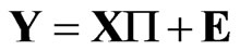 ,
, (1)
(1)
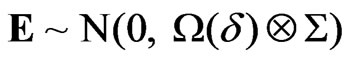
where Y and E are T × m random matrices, X is a T × k fixed design matrix, P is a k × m matrix of parameters, W (d) and S are T × T and m × m positive definite matrices, respectively, and d is the parameter of interest determining whether or not the columns of E are i.i.d. Tdimensional errors, i.e., W(d0) = IT. [17] found that the Locally Best Invariant (LBI) test statistic of the null hypothesis H0: d = d0 against the one-sided alternative H1: d > d0 has the following general expression
 (2)
(2)
where tr is the trace operator, Ê = MY is the residual matrix in the ordinary least squares regression of Y on X, M = IT – X(X¢X)–1 X¢ and K is the first derivative d W (d)/dd evaluated at d = d0. Invariance is defined against the group of transformations Y ® YP + XA for an arbitrary k × m matrix A and a positive definite m × m matrix P. Thus, without loss of generality, it can be assumed that S = IT. From [17], and following [1], it can also be proved that the LBIU test statistic of H0: d = d0 against the two-sided alternative H1: d ≠ d0 is given by (2) but with K being the second derivative d2W(d)/dd2 evaluated at d = d0.
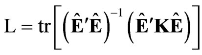
The null distribution of L can be characterized rewriting it as
 (3)
(3)
where lt are the non-null eigenvalues of the product matrix MK, et ~ N(0, Im), Bt ~ Beta (m/2, (T – k – m)/2) and B1 + … + BT–k = m, see, e.g., [20] p. 540. [17] found that the first two moments of L are given by
 and
and 
with c = 2m(T – k – m)/[(T – k – 1)(T – k + 2)] and
In the next section, we give formulae to compute tr (MK) and tr(MK)2 for some useful test statistics.
3. Test Statistics
3.1. Multivariate Seasonal Random Walk Plus Noise Model
[21] derived the LBI test statistic for a vector deterministic level in the multivariate local level model. We consider here the seasonal extension of this multivariate model given by
 ,
,  ,
,  , (4)
, (4)
where the vector time series yt = (y1t, …, ymt)¢ is decomposed into the sum of a vector seasonal random walk at = (a1t, …, amt)¢ plus a vector Gaussian white noise ut = (u1t, …, umt)¢ ~ N(0, S), the vector Gaussian white noise vt = (v1t, …, vmt)¢ ~ N(0, rS) is assumed to be independent of ut, and the parameter r > 0 quantifies the degree of stochasticity of at. Without loss of generality we assume that the seasonal period k is even and that the dataset is balanced, T = nk.
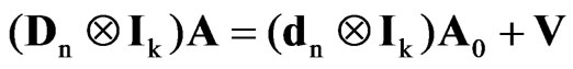
Defining the T × m matrices Y = [y1,…, yT]¢, A = [a1,…, aT]¢, U = [u1,…, uT]¢ and V = [v1, , vT]¢, (4) can be written in matrix form as
 ,
, (5)
(5)
where A0 = [a–k+1, …, a0]¢ is a k × m matrix of initial conditions, Ä denotes the Kronecker or tensor product, Dn is an n × n lower bidiagonal matrix with 1s on the main diagonal and –1s on the first sub-diagonal, which can be horizontally partitioned as Dn = [dn|Ñn]¢, being dn = (1, 0, …, 0)¢ and Ñn the (n – 1) × n first-order differencing matrix. If A0 is assumed to be fixed, it follows that (4) is a special case of (1) with
 ,
,  ,
, 
where , in = Cndn and X is a T × k matrix of seasonal dummy variables.
The LBI test statistic for testing the null hypothesis of deterministic seasonality (H0: r = 0) against the alternative of seasonal random walk (H1: r > 0), denoted by RWm,k,n, is given by (2) with
 (6)
(6)
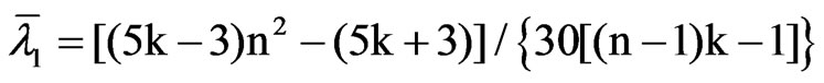
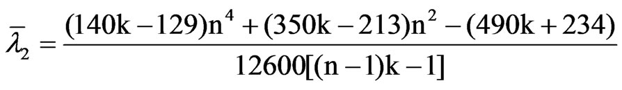
and Ê being the residual matrix in the multivariate regression of Y on the full set of k seasonal dummies. To compute the two first moments of , we find that the mean and mean-square of the eigenvalues of MK are given by
 and
and 
which suggest to correct the RWm,k,n test statistic by a factor depending of the sample size so that it converges to a non-degenerate limiting distribution. Some candidates are n, mn or m (n – k). It should be noted that RWm,k,n/mn has asymptotic mean 1/6 and variance 1/45 mk.
[21] also derived the LBI test statistic for a vector deterministic linear trend. We obtain here the LBI test statistic for a vector deterministic seasonal linear trend by including a vector seasonal drift βt in (4)
 ,
,  ,
, (7)
(7)
whose matrix form is given by
 ,
,

where B0 = [β–k+1, …, β0]¢ is a k × m fixed matrix of initial conditions for  If A0 is fixed, (7) is a special case of (1) with X = [in Ä Ik, tn Ä Ik], P = [A0, B0] and W(r) = IT + r(Cn
 Ä Ik), where tn = (1, 2, …, n)'. It is now clear that the inclusion of the vector seasonal drift only affects the mean vector of the sampling distribution of Y,
  , but not its covariance matrix. Therefore, the LBI statistic for testing the null hypothesis of vector deterministic seasonal linear trend (H0: r = 0) against vector seasonal drifted random walk (H1: r > 0) in (7), say DRWm,k,n, is computed as RWm,k,n, being now Ê the residual matrix in the multivariate regression of Y on k seasonal dummies and k seasonal lineal trends. We find for DRWm,k,n that the mean and mean-square of the eigenvalues of MK are given by
 and
and 
and so DRWm,k,n has asymptotic mean 1/15 and variance 11/6300 mk.
We also obtain another relevant modification of the RWm,k,n test statistic by including the time index t as a regressor in (4)
 ,
, (8)
(8)
or in matrix form,
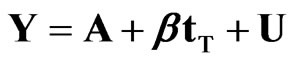 ,
, 
which is a special case of (1) with X = [in Ä Ik, tT], P = [A0, b0] and W(r) as in (7). By the same token, the LBI statistic for testing H0: r = 0 against H1: r > 0 in (8), say TRWm,k,n, is computed as RWm,k,n, being now Ê the residual matrix in the multivariate regression of Y on k seasonal dummies and a regular lineal trend. We find for TRWm,k,n that the mean and mean-square of the eigenvalues of MK are given by
and
It should be noted that DRW1,1,n = TRW1,1,n is the [3] test statistic for a univariate deterministic linear trend, and that the asymptotic mean and variance of TRW1,1,n/n are 1/15 and 11/6300, which agree with those obtained by [3] in a rather complicated proof.
3.2. Vector Seasonal IMA(1,1)k Model
Multivariate structural model (4) can be written as a vector seasonal IMA(1,1)k process
 ,
, (9)
(9)
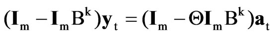
where B is the backshift operator such that Bkyt = yt–k, at = (a1t, …, amt)', Wa is a m × m positive definite matrix, and the parameter  is restricted to be positive so that ρ = (1 – Θ)2/Θ > 0. Process (9) is said to be invertible when Θ < 1 and strictly non-invertible when Θ = 1. In the last case, the cancellation of the matrix polynomials on both sides of the equation reveals the presence of deterministic seasonality. Noting that ρ(Θ) = ρ(1/Θ), the one-sided testing problem H0: r = 0 versus H1: r > 0 is equivalent to the two-sided one H0: Θ = 1 versus H1: Θ ≠ 1. Hence, the LBI test statistic RWm,k,n for a null variance ratio in (4) is the LBIU test statistic for strict noninvertibility in (9). Note that RW1,k,n is the [11] test statistic for a seasonal MA unit root.
Analogously, it can be proved that DRWm,k,n and TRWm,k,n are the LBIU test statistics of H0: Θ = 1 versus H1: Θ ≠ 1 in the reduced form of (7),

and (8)

respectively. Note that DWR1,k,n is closely related to the [22] test statistic, while TRW1,k,n is the [12] test statistic for non-invertibility in the seasonal IMA(1,1)k model.
3.3. Dynamic Seasonal Linear Models
[6] considered testing the null hypothesis of deterministic seasonality against the alternative of mixed deterministic and stochastic seasonality. A related multivariate LBI test statistic can be derived in the seasonal linear regression
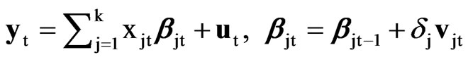 (10)
(10)
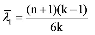
where xjt (j = 1, …, k) are a full set of seasonal dummy variables, βjt is either a time-varying parameter if dj = 1 or a nuisance constant parameter if dj = 0, ut ~ N(0, S), vjt ~ N(0, (r/k)S) are mutually and serially uncorrelated vector errors, and is here divided by k for comparison purposes given that (10) reduces to (4) when d1 + … + dK = k. Assuming that the initial conditions β1,0, …, βk,0 are fixed, (10) is a special case of (1) with X = [x1, …, xk]', P = [β1,0, …, βk,0]' and W(r') = IT + r'(dA1 + … + dkAk), where xj = (xj1, …, xjT)', Aj = xj°CTC'T°xj, and the operator denotes the Hadamard product. The LBI test statistic for testing the null hypothesis of deterministic seasonality (H0: d1 + … + dk = k) against the alternative hypothesis of mixed deterministic-stochastic seasonality (H1: d1 + … + dk = r < k), say SDm,k,n (r), is given by (2) with K = (dA1 + … + dkAk)/k, which coincides with RWm,k,n when r = k. Noting that MAjMAi = 0 for j ≠ i, we find that the eigenvalues of MK have mean and mean-square are given by
 and
and 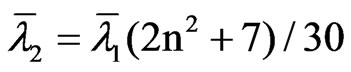
Analogously, when the explanatory variables in (10) are trigonometric seasonal variables (x1t = 1, xjt = cos(jtπ/k) for j even, and xjt = sin[(j – 1)tπ/k] for j odd and j > 1), it is convenient to assume that vjt ~ N(0, rjS), where rj = ajr/k2 with aj = 1 (j = 1, k) and aj = 2 (j = 2, …, k – 1). Now, as before, (10) reduces to (4) when r = k. Here, we can focus our attention on testing the deterministic or stochastic nature of the local level β1t, the (j/2)-th harmonic βjtcos(πjt/k) + βj+1,tsin(πjt/k) (j = 2, 4, …, k) or any combination of these k/2 harmonics. Taking as illustration the (j/2)-th harmonic, the LBI test statistic for testing the null hypothesis of deterministic seasonality (H0: d1 + … + dk = k) against the alternative of mixed deterministic-stochastic seasonality (H1: d1 + … + dk = 2) is given by (2) with K = aj (Aj + Aj+1)/k2 with Aj as defined before. We find that the eigenvalues of MK have mean and mean-square given by
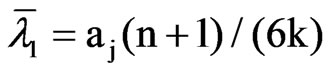
and
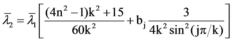
where bj = 0 (j = 1, k) and bj = 1 (j = 2, …, k – 1). Note that these expressions are also valid to compute the mean and variance of the LBI test statistic for a deterministic level in presence of deterministic seasonality, H0: r = 0 versus H1: r > 0, which is closely related to the KPSS test with seasonal dummies proposed by [23]. Furthermore, [7,8] derived the LBI test statistic, say TV1,k,n, for the dual testing problem of deterministic seasonality in presence of a deterministic level, which was generalized to the multivariate case by [16]. This test statistic is given by (2) with K = (a2A2 + … + akAk)/k2. We find that the eigenvalues of MK have mean and mean-square given by
 and
and 
4. Approximate Distributions and Accuracy
4.1. Asymptotic Samples
Following [11] and [21], it can be shown that the limiting distribution of RWm,k,n/mn under testing H0: r = 0 is
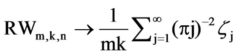 (11)
(11)
where ξj ~ iid . [2] noted that RW1,1,n/n follows the same limiting distribution as the Cramèr-von Mises goodness-of-fit test statistic. Hence, (11) is the average of mk copies of the Cramèr-von Mises distribution, denoted by CvM(mk)/mk. [24] found that the first four cumulants of a CvM(r) distribution are given by
 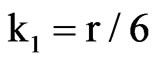 ,
,  ,
,  ,
,  which reveal that the distribution is strongly rightskewed and leptokurtic. We observe that the two parameter Inverse Gaussian distribution, IG(µ, λ), can be fitted to possess similar characteristics. The first four cumulants of this distribution are
  ,
,  ,
, 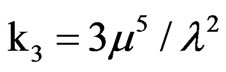 ,
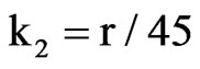
, 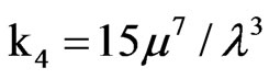 and matching the first two cumulants, μ = r/6 and μ3/λ= r/45, we obtain that the fitted IG(r/6, 45r2/63) distribution has third and fourth cumulants given by κ3 = 8r/900 and κ4 = 8r/1350, which seem to be quite close to those of the CvM (r) distribution. The accuracy of the IG approximation is illustrated in Figure 1, which shows the limit pdf of RW1,1,n/n evaluated by the [13] procedure (solid line), along with the pdf of the fitted IG(µ, λ) distribution (dashed line) given by

with x > 0, μ = 1/6 and λ = 45m/63. We can see that the IG approximation provides a very good fit on both tails
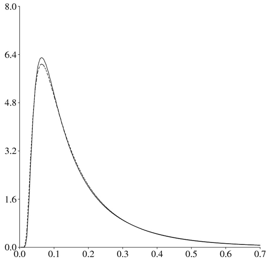
Figure 1. Accuracy of the IG approximation.
of the distribution. Therefore, accurate asymptotic pvalues for RWm,k,n/mn can be computed from the cdf of the IG(µ, λ) distribution.
4.2. Finite Samples
The goodness-of-fit in the asymptotic case take us to ask if the approximation will be also good in finite samples. To evaluate the exact null distribution of RWm,k,n/mn from (3)-(6), we must determine the eigenvalues of the matrix MK. To this end, it is convenient to note that the projection matrix M can be alternatively written as M = [Ñ¢n(ÑnÑ¢n)–1Ñn] Ä Ik. Hence, MK = (ÑnÑ¢n)–1 Ä Ik and its eigenvalues are the reciprocals of those of the tridiagonal matrix ÑnÑ¢n, λt = [4sin2(tπ/2n)]–1 (t = 1, 2, …, n – 1), each one with multiplicity k. In the case m = 1, (3)-(6) can be expressed as a ratio of quadratic forms in normal variables whose distribution was tabulated by [11] using the [13] procedure (they used n – 1 as correction factor instead of n). However, when m > 1, similar tables can be obtained by Monte Carlo simulation from (2)-(6).
To assess the accuracy of the IG approximation in small samples we simply compare the approximate pvalues with the nominal sizes for n = 10, 20, 30, 50 10, k = 1, 2, 3, and m = 1, 2, 3, 4, 5. In general, the approximate p-values agree closely with the nominal sizes even in small samples, being the mean absolute errors less than 0.003. Such discrepancies seem not to be relevant in practical applications. Similar results have been found for DRWm,k,n and TVm,k,n. The results of this simulation study are not presented here due to space restrictions but are available from authors at request.
5. Conclusions
We have presented seasonal extensions of the [21] test for a deterministic level in multivariate models that can be used to detect different forms of non-invertibility in VARIMA models. The two-moment IG approximation to the null distribution of these test statistics, along with the closed forms expressions for the first two moments here derived, provide a simple and fast way to compute accurate critical values and p-values in practical applications. The proposed approximation could be also useful when modifying the test statistics to deal with intervention variables and serially correlated errors. Finally, the testing procedures described have been implemented in a computer program that can be freely obtained from authors at request.
6. References
[1] M. L. King and G. H. Hillier, “Locally Best Invariant Tests of the Error Covariance Matrix of the Linear Regression Model,” Journal of the Royal Statistical Society, Series B (Methodological), Vol. 47, No. 1, 1985, pp. 98- 102.
[2] J. Nyblom and T. Mäkeläinen, “Comparisons of Tests for the Presence of Random Walk Coefficients in a Simple Linear Model,” Journal of the American Statistical Association, Vol. 78, No. 384, 1983, pp. 856-864. doi:10.2307/2288196
[3] J. Nyblom, “Testing for Deterministic Linear Trend in Time Series,” Journal of the American Statistical Association, Vol. 81, No. 394, 1986, pp. 545-549. doi:10.2307/2289247
[4] D. Kwiatkowski, P. C. B. Phillips, P. Schmidt and Y. Shin, “Testing the Null Hypothesis of Stationarity against the Alternative of a Unit Root,” Journal of Econometrics, Vol. 54, No. 1-3, 1992, pp. 159-178. doi:10.1016/0304-4076(92)90104-Y
[5] J. Nyblom and A. Harvey. “Testing against Smooth Stochastic Trends,” Journal of Applied Econometrics, Vol. 16, 2001, pp. 415-429. doi:10.1002/jae.604
[6] F. Canova and B. E. Hansen, “Are Seasonal Patterns Constant over Time? A Test for Seasonal Stability,” Journal of Business and Economic Statistics, Vol. 13, No. 3, 1995, pp. 237-252. doi:10.2307/1392184
[7] M. Caner, “A Locally Optimal Seasonal Unit-Root Test,” Journal of Business and Economic Statistics, Vol. 16, No. 3, 1998, pp. 349-356. doi:10.2307/1392511
[8] F. Busetti and A. Harvey, “Seasonality Tests,” Journal of Business and Economic Statistics, Vol. 21, No. 3, 2003, pp. 420-436. doi:10.1198/073500103288619061
[9] K. Tanaka, “Testing for a Moving Average Unit Root,” Econometric Theory, Vol. 6, No. 4, 1990, pp. 433-444. doi:10.1017/S0266466600005442
[10] P. Saikkonen and R. Luukkonen, “Testing for a Moving Average Unit Root in Autoregressive Integrated Moving Average Models,” Journal of the American Statistical Association, Vol. 88, No. 422, 1993, pp. 596-601. doi:10.2307/2290341
[11] W. Tam and G. C. Reinsel, “Tests for Seasonal Moving Average Unit Root in ARIMA Models,” Journal of the American Statistical Association, Vol. 92, No. 438, 1997, pp. 725-738. doi:10.2307/2965721
[12] W. Tam and G. C. Reinsel, “Seasonal Moving-Average Unit Root tests in the Presence of a Linear Trend,” Journal of Time Series Analysis, Vol. 19, No. 5, 1998, pp. 609-625. doi:10.1111/1467-9892.00112
[13] J. P. Imhof, “Computing the Distribution of Quadratic Forms in Normal Variables,” Biometrika, Vol. 48, No. 3-4, 1961, pp. 419-426. doi:10.1093/biomet/48.3-4.419
[14] R. B. Davies, “Numerical Inversion of a Characteristic Function,” Biometrika, Vol. 60, No. 2, 1973, pp. 415-417. doi:10.1093/biomet/60.2.415
[15] T. W. Anderson and D. A. Darling, “Asymptotic Theory of Certain ‘Goodness of Fit’ Criteria Based on Stochastic Processes,” The Annals of Mathematical Statistics, Vol. 23, No. 2, 1952, pp. 193-212. doi:10.1214/aoms/1177729437
[16] F. Busetti, “Tests of Seasonal Integration and Cointegration in Multivariate Unobserved Component Models,” Journal of Applied Econometrics, Vol. 21, 2006, pp. 419- 438. doi:10.1002/jae.852
[17] J. Nyblom, “Invariant Tests for Covariance Structures in Multivariate Linear Model,” Journal of Multivariate Analysis, Vol. 76, 2001, pp. 294-315. doi:10.1006/jmva.2000.1918
[18] J. MacKinnon, “Approximate Asymptotic Distribution Functions for Unit-Roots and Cointegration Tests,” Journal of Business and Economic Statistics, Vol. 12, 1994, pp. 167-176. doi:10.2307/1391481
[19] J. A. Doornik, “Approximation to the Asymptotic Distributions of Cointegration Tests,” Journal of Economic Surveys, Vol. 12, 1998, pp. 573-593. doi:10.1111/1467-6419.00068
[20] C. R. Rao, “Linear Statistical Inference and its Applications,” 2nd Edition, Wiley, New York, 1973. doi:10.1002/9780470316436
[21] J. Nyblom and A. Harvey, “Tests of Common Stochastic Trends,” Econometric Theory, Vol. 16, 2000, pp. 176-199. doi:10.1017/S0266466600162024
[22] A. M. R. Taylor, “Locally Optimal Tests against Unit Roots in Seasonal Time Series Processes,” Journal of Time Series Analysis, Vol. 24, No. 5, 2003, pp. 591-612. doi:10.1111/1467-9892.00324
[23] P. C. B. Phillips and S. Jin, “The KPSS Test with Seasonal Dummies,” Economics Letters, Vol. 77, 2002, pp. 239-243. doi:10.1016/S0165-1765(02)00127-1
[24] B. M. Brown, “Cramèr-Von Mises Distributions and Permutation Tests,” Biometrika, Vol. 69, No. 3, 1982, pp. 619-624.