Open Journal of Geology
Vol.4 No.8(2014), Article ID:48517,10 pages
DOI:10.4236/ojg.2014.48027
Spatial Variability of Shear Wave Velocity Using Geostatistical Analysis in Mashhad City, NE Iran
Azam Ghazi, Naser Hafezi Moghadas*, Hossein Sadeghi, Mohammad Ghafoori, Gholam Reza Lashkaripour
Department of Geology, Faculty of Sciences, Ferdowsi University of Mashhad, Mashhad, Iran
Email: *nhafezi@um.ac.ir
Copyright © 2014 by authors and Scientific Research Publishing Inc.
This work is licensed under the Creative Commons Attribution International License (CC BY).
http://creativecommons.org/licenses/by/4.0/


Received 17 May 2014; revised 15 June 2014; accepted 10 July 2014
ABSTRACT
Shear wave velocity (Vs) is one of the most important parameters of a geological model to assess the site effect and the ground response. In this paper the spatial variability of shear wave velocity in Mashhad capital city are investigated. For this purpose, 243 Vs profiles of different projects throughout the city were used. Based on the Vs profiles the iso-level maps of the Vs interfaces 300, 500, 750, 950 and 1200 m/s were obtained by kriging interpolation method. The best semivariogram models were obtained with changing the effective parameters and assessing the components of the models and spatial dependence. The best models for the entire interfaces were exponential. Based on these models, the spatial dependence of depth data was moderate to strong. The performance of interpolations was checked by cross-validation and its indices i.e. mean standardized prediction errors (MSPR), root mean square prediction errors (RMSPE), average kriging standard error (AKSE), and root mean square standardized prediction errors (RMSSPE) were assessed. A trend of depth increasing towards the northeast was observed at all of the interfaces.
Keywords:Kriging, Interpolation Accuracy, Vs Interface, Mashhad City

1. Introduction
A geological model including the geometry of the basin, the soil structure and the dynamic properties of the soil layers with great attention to the shear wave velocity (Vs) is a fundamental requirement for site effect studies [1] . Many studies have been performed around the world to assess site effect using different methods of 1D, 2D or 3D geological models. For all the methods especially 2D and 3D, a precise model of the basin is the key to accurate predictions of the ground response [1] -[4] .
Geostatistical analyses are powerful tools to obtain a precise understanding of the basin characteristics. Geostatistical analyses help to estimate the value of sample properties at the unmeasured locations. There are different geostatistical techniques such as kriging, inverse distance weighting (IDW), splines and triangulation which convert the point data to continuous surfaces by using the spatial interpolation. Most of these methods assume that the adjacent samples tend to be more similar than those which are further apart. This assumption describes the spatial autocorrelation. Experimental semi-variogram can define the spatial structure of a variable [5] . Each geostatistical method has its own advantage and disadvantage, and numerous studies have been performed to find the best method. Chaplot et al. (2006) used various geostatistical techniques and concluded that IDW and kriging were better estimators in reigns with sparse information [6] . IDW employs a simpler spatial interpolation method than kriging and it does not require the spatial autocorrelation [7] . Kriging methods including simple, ordinary and indicator are very effective and reliable for modeling of geological characteristics and mining applications [5] [8] . In general, kriging is the best linear unbiased estimator which may be free from systematic error and have minimum variance [9] -[11] .
In this study, the spatial variability of the Vs throughout the Mashhad city is investigated by kriging technique. For this purpose, data of 243 Vs profiles which have been measure during the period of 2000-2014 are utilized. The accuracy of the interpolations is inspected by the cross-validation analysis.
2. Materials and Methods
2.1. Study Area
The Mashhad city is the second largest city of Iran with dense population and high seismicity; it is situated in the Northeast of Iran. The city (36˚18'N, 59˚34'E) is located in the northern slopes of Binalood Mountains and Paleo-Tethys suture zone. It covers an area of 311 km2 and is dominated by an arid and semi-arid climate. It is laid on thick Quaternary deposits which are surrounded by Mafic and Ultramafic outcrops in southern parts, Slate and Phyllite in western and southwestern and Marls in northeastern margins. The city is also located in active tectonic area and bounded with two active and quaternary faults in south and north. The soft sediments are divided into three groups of pediment, alluvial fan and alluvial plain deposits. Pediment and alluvial fan deposits generally contain gravels and sands and extent over the south, southwest and west parts of the city. Alluvial plain deposits usually consist of clays and silts that cover center and eastern parts. Kashafrood River passing through the Northeast margin has significant effects on depositional process of the fine grained deposits and is the most important geomorphic phenomenon of the Mashhad watersheds. The highest part of the city with elevation of 1380 m.a.s.l. is lying in the southwestern outcrops. The lowest part of the city with altitude of about 870 m lies in the northeast. Almost 85% of the city have gradient slope less than 5 percent. Rivers which originated from the southern and southwestern outcrops flow towards the lowlands in the northeast and go into the Kashafrood River.
Physical and mechanical properties of the soft sediments in the study area are influenced by geological condition. Borehole logs of 1500 geotechnical boreholes collected from the city show that the soil texture in the south and south west are gravel and sand but gradually change to silt and clay toward north and east.
2.2. Shear Wave Velocity and Soil Texture Information
We utilized the shear wave velocity information of 243 boreholes. These boreholes were drilled during geotechnical studies for different projects such as hotels, residential and commercial buildings. Downhole shear wave profiling has been done by Zamin Physics Consulting Engineering Company. Mashhad is spiritual capital of Iran and more than 20 million tourists and pilgrims visit the city annually. Hence tendency increases to construct highraised commercial buildings, malls, and hotels. The main aim of downhole Vs measuring are determining seismic soil classification based on 2800 Iranian Seismic Code. Most of the boreholes were drilled to depth of 30 m although some continue more than 30 meters. The Vs profiles scattered throughout the city are shown in Figure 1.
2.3. Method
In the area under study, because special sedimentary environment texture and geotechnical properties of the soil
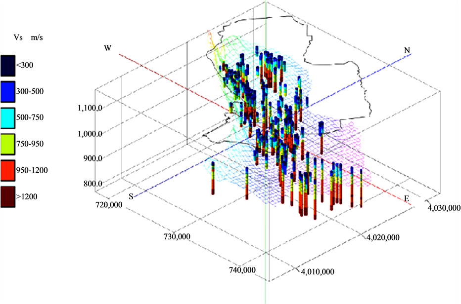
Figure 1. Vs profiles distributed around the city. Cold colors indicate low velocity and hot colors demonstrate high velocity.
change from point to point and finding a continuous layer is very difficult. Hence, we use shear wave velocity to determining the soil layers and construction of the basin model. The Vs information is considered as a base of model and the dominant soil texture is used for more detailed layer separation. For this firstly, variation of the Vs at different depths was discovered by the stock chart. Based on the stock charts, 5 breaking points at the Vs of 300, 500, 750, 950 and 1200 m/s were determined visually as seen in Figure 2. The Vs breaking points are used as the base of Vs iso-level maps. Then, the related depths of each breaking point were determined in all Vs profiles. Finally, kriging technique is used to interpolate the iso-level of the Vs interfaces.
More detailed information about the geostatistical techniques are noted in literature [7] [12] . Hence, we briefly describe the kriging method. Kriging [13] is a well-known technique in geostatistical interpolation methods. This method is based on the weighted moving average logic. The estimate values at the unmeasured locations are calculated by weighted sums of the adjacent measured values as follow:
 (1)
(1)
where
 is the estimated value of variable at unmeasured location
 ,
,
 is the value of the variable at this location,
 is the weight of measured
 value, and
![]() is the number of adjacent data contributed in estimation. The weights are estimated
by semivariogram (variogram). Semivariogram is a key tool to determine spatial structure
that is function of distance and degree of spatial variability and defined as [14] :
is the number of adjacent data contributed in estimation. The weights are estimated
by semivariogram (variogram). Semivariogram is a key tool to determine spatial structure
that is function of distance and degree of spatial variability and defined as [14] :
 (2)
(2)
 and
and
 are the measured value of the regionalized variable at location of
 and
and
 respectively,
![]() is the number of data pairs separated by the distance of
is the number of data pairs separated by the distance of . Experimental semivariograms
are defined as plotting
. Experimental semivariograms
are defined as plotting
 versus the distance
 . These semivariograms are fitted by appropriate
mathematical models. In this study a Jack-knifing procedure used to find the best
model. This is a trial and error method, which used until a best fit between the
estimated and measured values was gained [15]
.
. These semivariograms are fitted by appropriate
mathematical models. In this study a Jack-knifing procedure used to find the best
model. This is a trial and error method, which used until a best fit between the
estimated and measured values was gained [15]
.
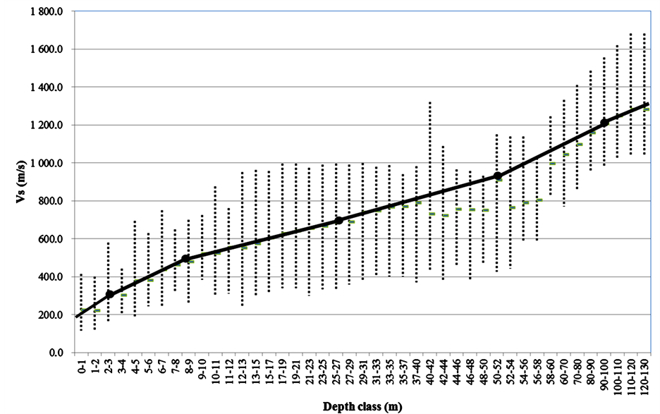
Figure 2. Stock plot of Vs against depth class, breakpoints are given by black solid circles.
Components of a semivariogram are including nugget effect, sill and range. Range
is the distance beyond which there is no spatial dependence and correlation between
data set points. Nugget effect
 shows the dissimilarity at the distances which are shorter than the measured variable
resolution and indicates the degree of spatial correlation. The nugget will be reduced
by decreasing the probability of random distribution of the variable and increasing
the spatial correlation. The sill
shows the dissimilarity at the distances which are shorter than the measured variable
resolution and indicates the degree of spatial correlation. The nugget will be reduced
by decreasing the probability of random distribution of the variable and increasing
the spatial correlation. The sill
 is the value of
 at which the semivariogram model flattens out [16]
.
at which the semivariogram model flattens out [16]
.
In this study, spherical, Gaussian and exponential models were considered to find the best semivariogram models. Spatial dependency is a way to recognize appropriate model [17] . It is defined as the ratio of the nugget to the sill and is expressed in percentage. Spatial dependency of a variable would be strong if the ratio was less than 25%, a ratio between 25% - 75% shows moderate spatial dependency of the variable, and the ratio of more than 75% implies on weak spatial dependence.
Cross-validation was also performed to evaluate the validation and adequacy of the semivariogram model [18] . This is a leave-one-out method that helps to assess the fitted model, appropriate number of the neighboring data for contributing at estimation and type of kriging [19] [20] . Validation of an interpolation was evaluated by comparing estimated and actual measured values [19] [21] . Four indices are used for assessing the validation. These are computed as follows:
Mean standardized prediction errors (MSPR),
 (3)
(3)
Root mean square prediction errors (RMSPE),
 (4)
(4)
Average kriging standard error (AKSE),
 (5)
(5)
Root mean square standardized prediction errors (RMSSPE),
 (6)
(6)
where
![]() is the number of locations
is the number of locations ,
,
 is the predicted value from cross-validation,
 is measured value and
 is the prediction standard error for location
 .
.
For an accurate interpolation the mean MSPR value must be near to zero, the RMSPE value should be small and AKSE value should be near to RMSPE, and the RMSSPE has to be near to 1 (ArcGIS Tutorial).
3. Results and Discussion
Classical statistical analysis for the depth variation of the Vs interfaces of 300, 500, 750, 950 and 1200 m/s were performed and the results including min, max, mean, median, Standard deviation (SD), skewness and kurtosis are presented in Table1 Minimum value of the occurrence depth of 300, 500, and 750 m/s interfaces is equal to zero, which belong to southern part of the city, close to outcrops. The interfaces of 300, 500 and 750 m/s are located in shallow depths, as average positioned depth of these interfaces were 4, 13, and 25 meters, respectively that could be attributed to the stiff soils and arid climate of the Mashhad city. It observed we received to interface of 750 m/s at shallow depths. Maximum depth occurrence of this interface was 45 m, which was observed at eastnorthen part of the city, where fine grain soils were predominant. The Vs change exponentially with depth throughout the Msahhad area [22] which could be the reason of deep interface of 950 and 1200 m/s. In general, variation of depth occurance of Vs interfaces became more by increasing the Vs minimum (2.2) and maximum (32.4) values of standard deviation are belonging to the 300 and 1200 m/s interfaces, respectively.
Normality of the data distribution is required for kriging interpolation. In this study the graphical histogram and Q-Q plot tests were used to analyze the normality. The depth information is normally distributed for the entire interfaces.
Among kriging methods, including simple, ordinary, universal, indicator, probability and disjunctive, we chose the ordinary kriging. Ordinary kriging is the most often used type of kriging and also the simplest with fewest required parameters.
We need appropriate semivarigram model for interpolating by kriging technique. For this, the effective parameters e.g. the lag size, the search direction, and the anisotropy must be selected. These parameters have great influence on the values of sill, nugget, range and the percent ratio of nugget to sill. The spatial dependence was used to select the great semivariogarm models. The exponential models were determined as the best models for all Vs interfaces. The extracted parameters from determined models are presented in Table2 The spatial dependences are varied from 0% to 27% and shown the moderate spatial dependence at the interfaces of 300 and 500 m/s and strong spatial dependence for the 750, 950 and 1200 m/s interfaces. In exception of 1200 m/s interface, Nugget and sill increase with velocity which may be influenced by high overburden stress.
We also examined the anisotropy on semivariogram modeling. The results indicate the anisotropy on data. As shown in Table 2, the most isotropy in data for 300 m/s interface occurred in direction about 70 degree but for others interfaces are about 120 degree. It indicates that the depositional trend for deep and old sediments were SW-NE in concordance with the main drainage of Kashafroud area; but it change to N-E for upper and young sediment. The effective range for the 300 and 500 m/s interfaces are 6 km and increase for other interfaces.

Table 1. Statistical parameters of interface depth values for all of the interfaces.
Table 2. Geostatistical parameters of fitted semivariogram models.
Large range value is related to the higher spatial structure. Other effective parameters for performing accurate interpolation are the number of neighbors and sector type.
The interpolation performances are analysis by plotting the predicted values versus
the measured values and also by cross-validation index
[18] . In Figure 3, the predicted values
of interface depth are plotted against measured values for all the interfaces and
the regression lines are compared with 1:1 line. Kriging estimator for all of the
interfaces seemed to overestimate the lower values and underestimate the values
of the higher depth. The reason could be the nature of kriging algorithm that aimed
to achieve unbiased predictions of the mean values. The slope of the linear regression
lines for 300, 500, 750, 950 and 1200 m/s interfaces is equal to 0.457, 0.505, 0.555,
0.831, and 0.941, respectively. The linear regression lines of the interfaces of
950 and 1200 m/s have steeper slope with higher
 equal to 0.71 and 0.86, respectively. A few data points are laid outside the 95%
confidence intervals, which differed for the different Vs interfaces. The confidence
intervals of the 950 and 1200 m/s interfaces are narrower than other interfaces
and the scatters are tighter. It shows the better prediction.
equal to 0.71 and 0.86, respectively. A few data points are laid outside the 95%
confidence intervals, which differed for the different Vs interfaces. The confidence
intervals of the 950 and 1200 m/s interfaces are narrower than other interfaces
and the scatters are tighter. It shows the better prediction.
The cross-validation indexes of interpolations, the MSPR, RMSPE, AKSE, and PMSSPE are shown in Table 3 for all of the interfaces. The MSPRs for all of the interpolation interfaces are close to zero, which demonstrates that kriging was relatively unbiased in interpolating the depth values of Vs interfaces. The MSPR of interpolations of Vs interfaces increased in order of 750, 500, 300, 950, and 1200 m/s interfaces. The values of the RMSPE and AKSE for all of the interpolations are close to each other, but they are not very small and increase with increasing the velocity of the interfaces. Since the average kriging standard error (AKSE) is lower than the RMSE, the kriging variance is less than the true estimation variance and indicates that the semvariogram models are overestimating the variability of the predictions. The RMSSPEs are all close to 1 that indicates the accuracy of interpolations. The closest RMSSPE to 1 was attained for 750 m/s (1.018) interface, which was better and fallowed by 500 m/s (1.065), 300 m/s (1.078), 950 m/s (1.095), and 1200 m/s (1.131) interfaces. The RMSSPE values are greater than 1, which indicted the underestimated of the variability in the predictions. In general, the accuracy of 3 top interface interpolations is more than bottom interfaces. It could be related to the less number of measured locations, which in spite of having the better regression lines decrease by increasing the velocity.
Kriged maps of the velocity interfaces and the attributed best fitted variogram are shown in Figure 4. In all maps deep areas are shown by dark brown color and shallow parts are indicated by light brown color. The depth of 300 m/s interface varied from 0 to 12 m. The lower values are belonging to the southern part of the city near to the outcrops and the higher values are related to the eastern and northeastern parts of the city which covers by the fine grained soils. As seen in subfigure (a) for the great part of the city, 300 m/s interface are located in depth of less than 5 m. It could be related to stiff soils that are covers the city. For all of the interfaces, a trend from the west and southwest toward east and northeast is available that is corresponded to the rivers streaming and getting finer of the soils. The interpolation map of 500 m/s interface is presented in subfigure (b) Deep areas are shown by dark brown color and shallow parts are indicated by light brown color. Based on this map, the depth to 500 m/s interface in the eastern part of the city is more than 15 m and in somewhere continues to 28 m. As seen in subfigure (c) a clear trend of depth increasing towards the northeast is available in 750 m/s interface. In this interface, about 20 percent of city from central to eastern part, next to the Kashafrood River, is laid on the depths of 30 - 40 m. The trend of depth increasing towards east and northeast is also observed in 950 m/s interface. Based on the subfigure (d) the difference between min and max depth is high and the depth varies from 15 to 90 m. The shallow parts with light brown color are laid near to south and southwest outcrops and the deep parts with dark brown color are located in the eastern and northeastern of the city. More than two thirds of 1200
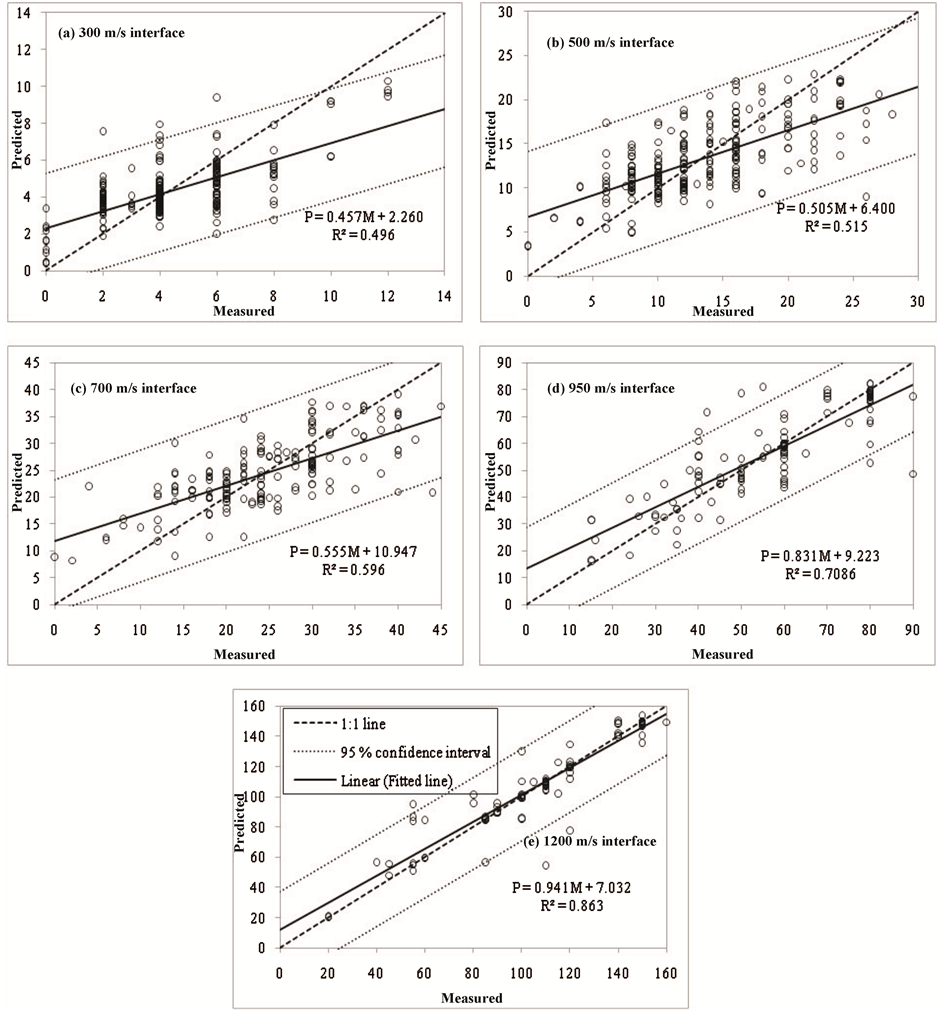
Figure 3. Cross-validation scatter plots of the interface depth values.
Table 3. Cross-validation indices of the interface depth values.
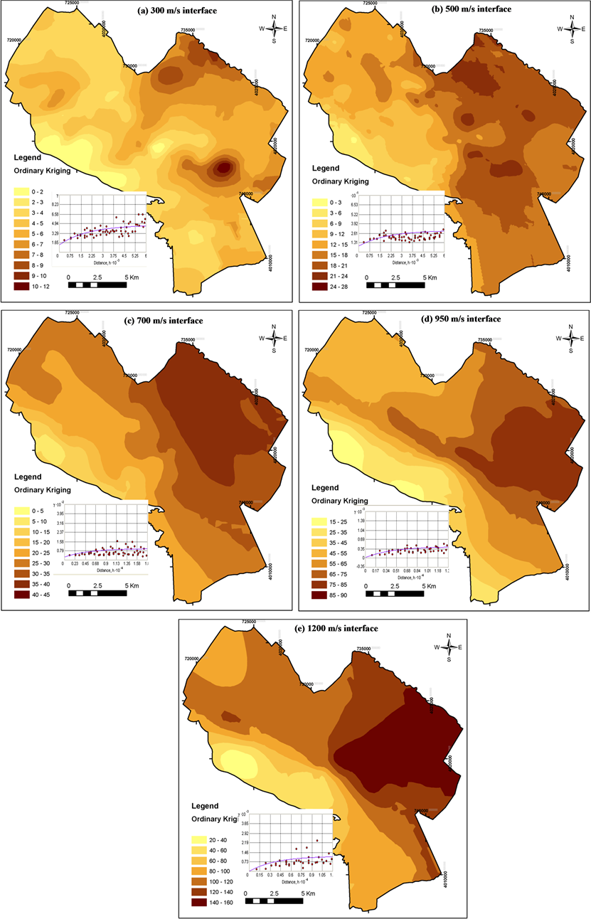
Figure 4. Semivariograms and kriged maps of the interfaces depth.
m/s interface has depth of more than 80 m depth of the interface is continued to 160 m in eastern and northeastern city.
Clay and silt sediments are located in the central, east and northeast parts of the city. In addition the groundwater level ranges from 15 to 40 m in these regions. Hence these regions are covered by the softer soils and are formed deepest parts in all interfaces.
4. Conclusion
In this study, statistical analyses are done to interpolate the Vs interfaces occurrence depth at velocity of 300, 500, 750, 950 and 1200 m/s. It is found that ordinary kriging is the best estimator to find the best fitted semivariogram to depth data. The moderate spatial dependence is seen for the depth data of the 300 and 500 m/s interfaces and is observed strong spatial dependence for the depth data of the 750, 950 and 1200 m/s interfaces. The range of resulted semivariogram in various Vs interface is different. The highest range is observed in 750 m/s interface and the lowest range is belonging to 300 m/s interface. The most isotropy in data for 300 m/s interface observed in direction of about 70 degree but for others interfaces occurred in direction of about 120 degree. All of the Vs interfaces became deeper towards northeast. The shallow parts of the entire interfaces are located near the south and southwestern outcrops while the deep parts are laid at the central, eastern and northeastern city. It could be related to the existence of the fine grained soils and shallow groundwater level at these regions.
Acknowledgements
This research was supported by Zamin Physic Pouya consulting engineering company and authors would like to thank this support.
References
- Manakou, M.V., Raptakis, D.G., Chavez-Garci, F.J., Apostolidis, P.I. and Pitilakis, K.D. (2010) 3D Soil Structure of the Mygdonian Basin for Site Response Analysis. Soil Dynamics and Earthquake Engineering, 30, 1198-1211. http://dx.doi.org/10.1016/j.soildyn.2010.04.027
- Brocher, T. (2005) A Regional View of Urban Sedimentary Basins in Northern California Based on Oil Industry Compressional-Wave Velocity and Density Logs. Bulletin of the Seismological Society of America, 95, 2093-2114. http://dx.doi.org/10.1785/0120050025
- Magistrale, H., Layghlin, M.C. and Day, S. (1996) A Geology Based 3-D Velocity Model of the Los Angeles bAsin Sediments. Bulletin of the Seismological Society of America, 86, 1161-1166.
- Semblat, J.F., Khamb, M., Pararaa, E., Bardb, P.Y., Pitilakis, K., Makrad, K. and Raptakis, D. (2005) Seismic Wave Ampli?cation: Basin Geometry vs Soil Layering. Soil Dynamics and Earthquake Engineering, 25, 529-538. http://dx.doi.org/10.1016/j.soildyn.2004.11.003�
- Rota, M. (2007) Estimating Uncertainty in 3d Models Using Geostatistics. PhD Thesis, European School for Advanced Studies in Reduction of Seismic Risk (Rose School), University of Pavia, Italy.
- Chaplot, V., Darboux, F., Bourennane, H., Leguedois, S., Silvera, N. and Phachomphon, K. (2006) Accuracy of Interpolation Techniques for the Derivation of Digital Elevation Models in Relation to Landform Types and Data Density. Geomorphology, 77, 126-141. http://dx.doi.org/10.1016/j.geomorph.2005.12.010
- Isaaks, E.H. and Srivastava, R.M. (1989) An Introduction to Applied Geostatistics. Oxford University Press, Oxford, 561.
- Rahman, K.M. (2007) Settlement Prediction on the Basis of a 3D Subsurface Model, Case Study: Reeuwijk Area, the Netherlands. MSc Thesis, International Institute for Geo-Information Science and Earth Observation, Enschede, The Netherlands.
- Clark, I. (1979) Practical Geostatistics. Applied Science Publishers Ltd., London, 129.
- Al-Mashagbah, A., Al-Adamat, R. and Salameh, E. (2012) The Use of Kriging Techniques with in GIS Environment to Investigate Groundwater Quality in the Amman-Zarqa Basin/Jordan. Research Journal of Environmental and Earth Sciences, 4, 177-185.
- Akiska, S., Sayili, I.S. and Demirela, G. (2013) Three-Dimensional Subsurface Modeling of Mineralization: A Case Study from the Handeresi (Canakkale, NW Turkey) Pb-Zn-Cu Deposit. Turkish Journal of Earth Sciences, 22, 574-587.
- Journel, A.G. and Huijbregts, J.C.H. (1978) Mining Geostatistics. Academic Press, London, 600.
- Krige, D.G. (1951) A Statistical Approaches to Some Basic Mine Valuation Problems on the Witwatersrand. Journal of the Chemical, Metallurgical and Mining Society of South Africa, 52, 119-139.
- Goovaerts, P. (1997) Geostatistics for Natural Resources Evaluation. Oxford University Press, New York, 496.
- Bailey, T.C. and Gatrell, A.C. (1998) Interactive Spatial Data Analysis. Addison Wesley Longman, London.
- Iqbal, J., Thomasson, J.A., Jenkins, J.N., Owens, P.R. and Whisler, F.D. (2005) Spatial Variability Analysis of Soil Physical Properties of Alluvial Soils. Soil & Water Management & Conservation, 69, 1338-1350.
- Cambardella, C.A., Moorman, T.B., Parkin, T.B., Karlen, D.L., Turco, R.F. and Konopka, A.E. (1994) Field Scale Variability of Soil Properties in Central Iowa Soils. Soil Science Society of America Journal, 58, 1501-1511. http://dx.doi.org/10.2136/sssaj1994.03615995005800050033x
- Myers, D.E. (1991) Interpolation and Estimation with Spatially Located Data. Chemometrics and Intelligent Laboratory Systems, 11, 209-228. http://dx.doi.org/10.1016/0169-7439(91)85001-6
- Stone, M. (1974) Cross-Validation Choice and Assessment of Statistical Prediction. Journal of the Royal Statistical Society, 36, 111-147.
- Liu, Z.P., Shao, M.A. and Wang, Y.Q. (2013) Large-Scale Spatial Interpolation of Soil pH across the Loess Plateau, China. Environmental Earth Sciences, 69, 2731-2741. http://dx.doi.org/10.1007/s12665-012-2095-z
- Zhang, R., Kravchenko, A. and Tung, Y.K. (1995) Spatial and Temporal Distribution of Precipitation in Wyoming. 15th Proceeding of Annual American Geophysical Union Hydrology Days, Fort Collins, CO, AGU, Washington, DC, 377-388.
- Hafezi Moghaddas, N., Ghafoori, M. and Ghazi, A. (2007) Investigation of Empirical Relationship between Shear Wave Velocity and N-SPT throughout the Mashhad City. 25th Annual Meeting of Earth Sciences, 145-152.
NOTES

*Corresponding author.