Open Journal of Geology
Vol.4 No.7(2014), Article
ID:47965,11
pages
DOI:10.4236/ojg.2014.47023
Prediction of Shear Wave Velocity Using Artificial Neural Network Technique, Multiple Regression and Petrophysical Data: A Case Study in Asmari Reservoir (SW Iran)
Habib Akhundi1, Mohammad Ghafoori2, Gholam-Reza Lashkaripour2
1Geology Department, Ferdowsi University of Mashhad, International Branch, Mashhad, Iran
2Geology Department, Ferdowsi University of Mashhad, Mashhad, Iran
Email: Akhundi.habib@stu.um.ac.ir, ghafoori@um.ac.ir, lashkaripour@um.ac.ir
Copyright © 2014 by authors and Scientific Research Publishing Inc.
This work is licensed under the Creative Commons Attribution International License (CC BY).
http://creativecommons.org/licenses/by/4.0/


Received 5 May 2014; revised 1 June 2014; accepted 30 June 2014
ABSTRACT
Shear wave velocity has numerous applications in geomechanical, petrophysical and geophysical studies of hydrocarbon reserves. However, data related to shear wave velocity isn’t available for all wells, especially old wells and it is very important to estimate this parameter using other well logging. Hence, lots of methods have been developed to estimate these data using other available information of reservoir. In this study, after processing and removing inappropriate petrophysical data, we estimated petrophysical properties affecting shear wave velocity of the reservoir and statistical methods were used to establish relationship between effective petrophysical properties and shear wave velocity. To predict (VS), first we used empirical relationships and then multivariate regression methods and neural networks were used. Multiple regression method is a powerful method that uses correlation between available information and desired parameter. Using this method, we can identify parameters affecting estimation of shear wave velocity. Neural networks can also be trained quickly and present a stable model for predicting shear wave velocity. For this reason, this method is known as “dynamic regression” compared with multiple regression. Neural network used in this study is not like a black box because we have used the results of multiple regression that can easily modify prediction of shear wave velocity through appropriate combination of data. The same information that was intended for multiple regression was used as input in neural networks, and shear wave velocity was obtained using compressional wave velocity and well logging data (neutron, density, gamma and deep resistivity) in carbonate rocks. The results show that methods applied in this carbonate reservoir was successful, so that shear wave velocity was predicted with about 92 and 95 percents of correlation coefficient in multiple regression and neural network method, respectively. Therefore, we propose using these methods to estimate shear wave velocity in wells without this parameter.
Keywords:Shear Wave Velocity, Petrophysical Logs, Neural Networks, Multiple Regression, Asmari Reservoir

1. Introduction
Yet, natural complexity of hydrocarbon reservoirs system is an important challenge in earth sciences. Lack of reliable information results in an appropriate understanding of reservoirs behavior and therefore leads to poor predictions of geomechanical and reservoir parameters. In the last decades, classical dada processing tools and physical models were sufficient to solve relatively simple geology issues, but today we are dealing with more complex problems and relying on existing techniques, which are based on common methods. They are less satisfactory [1] . Shear wave velocity is one of the most important parameters in exploratory studies of petroleum and gas industry which unfortunately hasn’t been measured in most wells due to high costs. For this reason, numerous methods have been presented to estimate these parameters from other well logging data that are recorded in most wells. Since shear wave velocity is affected from different parameters of the rock (compressional wave velocity, pore fluid and etc.) it could also indicate the physical properties of the rock. Hence, shear wave velocity is used in determining the type of lithology, pore fluid and geomechanical parameters of the formation such as shear modulus, bulk modulus and etc. [2] . So far, numerous empirical relationships have been presented for calculating shear waves velocity but, in most cases, the results of these relationships aren’t desirable in different areas due to following reasons:
1) Various parameters affect the shear wave velocity, and all of them aren’t included in empirical relationships; 2) Mentioned relationships belong to a particular area or reservoir rock (with specific lithology and fluid) and using these relationships in other areas doesn’t present a good response because the rock and fluid properties change; 3) Most of performed studies in order to measure the shear wave velocity have been about sandstones and little studies have examined the carbonate rocks, while most of Iran reservoirs are in carbonate type and thus further studies is required on petrophysical parameters of carbonate rocks.
Dipole Shear Sonic Imager (DSI) is a new tool that directly measures the shear wave velocity, but data of this tool isn’t available in all well especially old wells. Therefore, researchers try to estimate these parameters from other methods with acceptable accuracy. Importantly, the methods used in estimating these parameters first should be economic and secondly should not need new information. Well logging information such as porosity log is available in most wells. One of the benefits of these logs compared to other information is that in most cases they are continuously recorded throughout the well [3] . Therefore researches have always tried to integrate this information with other methods in order to obtain new information by spending minimum cost. Some of these methods are new statistical techniques and artificial neural networks which could solve issues related to reservoir characteristics and geomechanical parameters that old calculations can’t solve. Because of unique capabilities of neural network approach, it became a computational tool in petroleum industry. In studying Asmari reservoir which is a carbonate oilfield in the Zagros basin (south west of Iran), three wells have been selected among which two wells have shear wave velocity  data, compressional wave velocity and data related to petrophysical logs, but the third well hasn’t
  data. Thus prediction of
  in the third well, which has generalization capability to entire field, was carried out using other logs.
2. Compressional and Shear Waves
Bulk waves play an important role in petro-acoustical studies and are divided into two categories: compressional waves and shear waves. Relationship between velocity of compressional and shear waves with density and elastic coefficients is expressed as follow:
 (1)
(1)
 (2)
(2)
where  is compressional wave velocity,
  is shear wave velocity,
 ![]() is rock density,
is rock density, ![]() is stiffness modulus and
is stiffness modulus and ![]() is Lame constant. One of the most important properties of shear wave is that it cannot travel through the fluids, so it plays a major role in describing reservoir properties. Some of the important applications of shear waves are: 1) Lithology recognition:
is Lame constant. One of the most important properties of shear wave is that it cannot travel through the fluids, so it plays a major role in describing reservoir properties. Some of the important applications of shear waves are: 1) Lithology recognition:  is an index ratio that has certain value for different rocks (e.g. dolomite (1.9), Limestone (1.8), shale sand (1.7), and clean sand (1.6)); 2) Recognizing degree of consolidation (e.g. for recognizing the problem of sand production in reservoir); 3) Detecting the type of formation fluid; 4) Determining rock mechanics parameters; 5) geophysical studies such as Amplitude Variation with Offset (AVO).
3. Relations between Shear Wave Velocity and Petrophysical Data
Due to complexity of relationship between  values with all properties of rock and fluid, only important and measurable parameters of rock and fluid properties (that could be obtained through well logging data) were selected as main input parameters of the model. Thus selected parameters should have a significant effect on
 .
.
3.1. Density Log
Density log has a direct relation with compressional and shear wave velocities (Figure 1). According to Equations (3) and (4), as the formation density increases,  and
and  increase too (Schlumberger Log Interpretation, 1989).
 (3)
(3)
where  is formation density (bulk density),
 ![]() is matrix density and
is matrix density and  is fluid density.
3.2. Neutron Log
Neutron Porosity indicates the formation hydrogen index, which is detected by Neutron tool [4] . Neutron Log indicates the formation Porosity. The more the Porosity of the formation is, the less the Velocity passing through the formation (Equation (4) and Figure 2).
 (4)
(4)
where  is formation porosity (that is measured by neutron tool),
  is fluid velocity and
  is rock matrix velocity. So in intervals with higher Porosity (higher Neutron Porosity), Shear and Compressional Wave Velocities decrease.
3.3. Sonic Log
Compressional wave velocity could easily be obtained from sonic log and according to the Equation (7). As shown in Figure 3, there is a (good conformity between  and
and  versus the depth. Figure 4 also shows a direct and linear relationship between
  and
and .
.
3.4. Gamma Log
Gamma log measures the formation radioactivity which obtained from Equation (5):
 (5)
(5)
where  is density of radioactive minerals,
  is minerals volume,
 ![]() is a radioactive factor that depends on radioactivity intensity of minerals and
is a radioactive factor that depends on radioactivity intensity of minerals and  is formation density. Thus, as the formation density increases, the gamma decreases and vice versa. As mentioned before, velocity depends on the formation density (Equations (3) and (4)), and as the formation density increases (gamma reduces), the velocity also increases and vice versa [5] . Thus, as the gamma increases, the velocity decreases (Figure 5 and Figure 6).
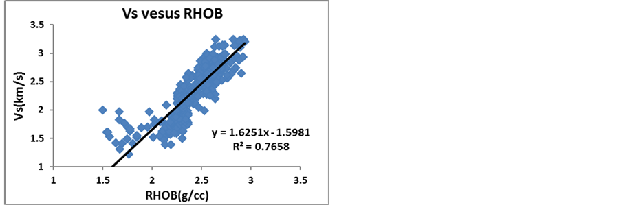
Figure 1. The relationship between shear wave velocity and formation density.
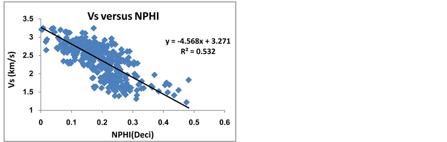
Figure 2. The relationship between shear wave velocity and neutron porosity.
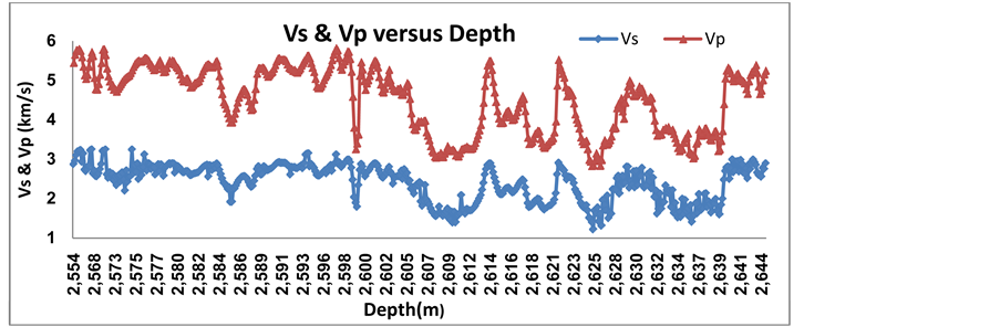
Figure 3. Comparison of shear and compressional wave velocities versus depth.
3.5. Resistivity Log
Figure 7 and Figure 8 show that shallow resistivity log  and deep resistivity log
  have nonlinear relationship with shear wave velocity. The following equation demonstrates the Archie formula [6] :
 (6)
(6)
where ![]() is formation resistivity,
is formation resistivity,  is formation water resistivity,
  is formation water salinity and
  is formation porosity. As is evident, with increasing of porosity, formation resistivity decreases, but we should consider effect of the fluid filling the pores, i.e. when hydrocarbon fills formation pores, resistivity increases and when the fluid filling the pores is water, depend on water salinity, resistivity decreases. As mentioned, the shear
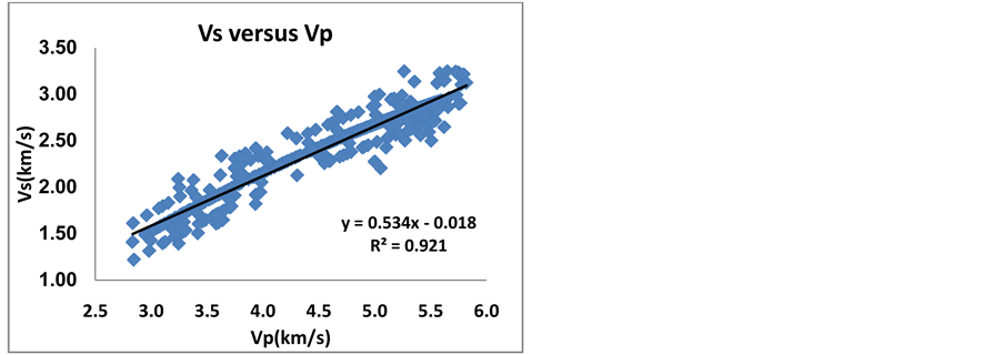
Figure 4. The relationship between shear wave velocity and compressional wave velocity.
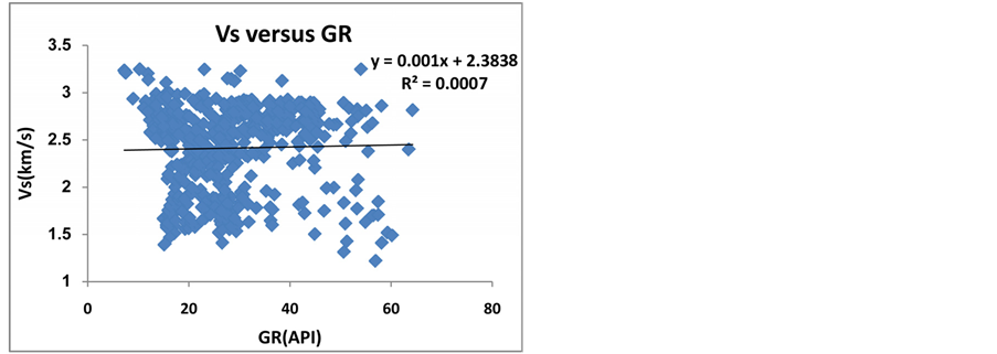
Figure 5. The relationship between shear wave velocity and gamma log.
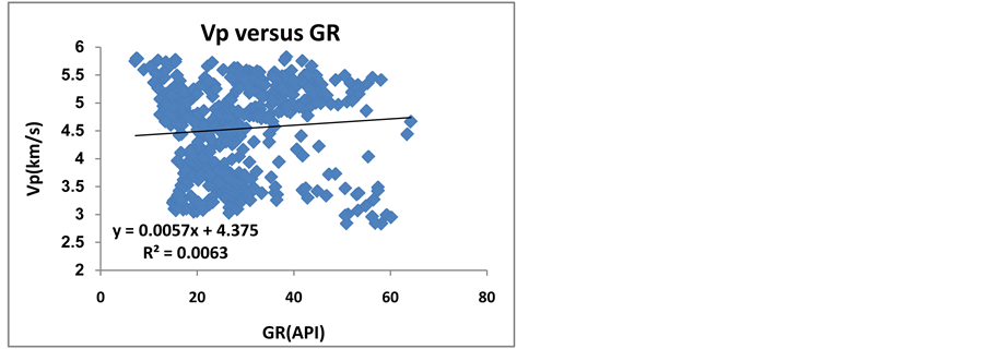
Figure 6. The relationship between compressional velocity and gamma log.
wave velocity is not influenced by this kind of fluid and doesn’t change with change of the fluid. Thus the shear wave velocity depends mainly on porosity effect and lithology type.
4. Results and Discussion
4.1. Castagna Method
There are different empirical equations (e.g. Han et al. 1986, Castagna et al. 1993, Pickett et al.) to predict ![]()
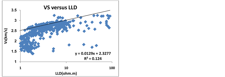
Figure 7. The relationship between shear velocity and deep resistivity log.
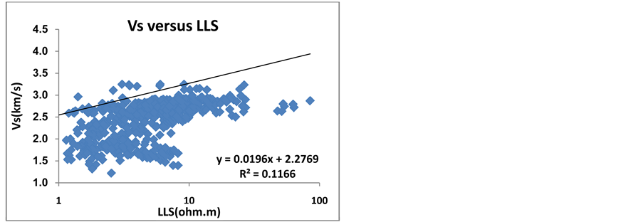
Figure 8. The relationship between shear velocity and shallow resistivity log.
using petrophysical log data [7] . We studied various empirical equations, which are a combination of different petrophysical parameters for predicting , In order to find out factors which have the most effect on
 . In addition, compare the relationship between shear wave velocity and other parameters and petrophysical logs
  showed that there is a close relationship between velocity of compressional and shear waves, especially in carbonate rocks (Figure 3 and Figure 4). Thus prediction of
  using compressional wave velocity is more reliable, especially in carbonate rocks. Given to the very close relationship of
  in carbonate rocks, among various empirical equations, we used Castagna equation to predict shear wave velocity. In the previous section, the effect of other features was determined through cross-plotting of these parameters versus
 . Generally, these empirical relationships only present good results in similar formations and their validation in other rocks is doubtful until it become calibrated. Thus providing a physical model that shows proper understanding of the shear wave behavior would be useful [8] .
In this study, compressional wave velocity  data has been obtained using sonic log
  data and through Equation (7). In addition Castagna et al. equations, which is used for limestone and dolomite, is presented below (Equations (8) and (9)):
 (7)
(7)
 (8)
(8)
![]() (9)
(9)
Figure 9 shows the result of comparison of  values, which measured and estimated by Castagna relationship for entire the reservoir. This relationship has an input parameter and correlation coefficient of
  values, which measured and estimated by Castagna relationship, is about 72%
 .
.
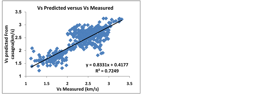
Figure 9. The measured shear wave velocity versus shear wave velocity estimated from Castagna relationship.
To increase the accuracy of the prediction  using regression, other parameters such as neutron porosity
 , density
 , gamma
 , deep resistivity log
  and shallow resistivity log
  were considered for entering to equation provided in the multiple regression. Figure 1, Figure 2 and Figures 5-8 show the effect of density, neutron, gamma, deep resistivity and shallow resistivity.
4.2. Multiple Regression Method
Multiple regression analysis uses from correlation between different well logging data and desired parameter. To estimate a parameter in multiple regression, initially this parameter is communicated to several other parameters. The advantages of this technique compared to simple regression are its more accuracy and its capability to summarize more information. It should be noted in using this technique that parameters which are selected for multiple regression should be independent from each other and don’t have a high correlation [9] . Although previous empirical studies present a proper instruction to select dependent variables, however new prediction equations should be presented for each new region or field. Therefore to identify input data, first we should determine the correlation coefficients between different well logging data by shear wave velocity. Then data that have the highest correlation with shear wave velocity are selected as input data. For this purpose, the correlation coefficients between different well logging data and shear wave velocity were calculated. Then data with high correlation coefficient were selected. According to Figures 1-8, parameters having the highest correlation coefficient with shear wave velocity are: data of compressional wave velocity, density, neutron porosity, deep and shallow resistivity and gamma ray.
These methods have errors and inaccuracies in the final response because of using assumptions which needed to derive the answer. These assumptions include homogeneity in depositional environment and existence of simple linear relationship between shear wave velocity and petrophysical parameters, so these six parameters (compressional wave velocity, density, neutron porosity, shallow and deep resistivity and gamma ray) can be used as input to multiple regression.
A multivariate model of the data solves for unknown coefficients  of a multivariate equation such as Equation (10):
 (10)
(10)
Weight of input variables to predict  is determined by contribution degree of
  (which characterized by multiple regression). After all variables
  were included in the model, the following equation with correlation coefficient of 90% was obtained.
 (11)
(11)
The above equation shows that the coefficients of independent variables  is high and they are important variables of the regression but coefficients of
  and
and ![]() is low and they are the weakest variables of the model. In this stage, Low-value variables (low coefficients) were removed from the model and the new model was fitted again and the following equation was obtained:
is low and they are the weakest variables of the model. In this stage, Low-value variables (low coefficients) were removed from the model and the new model was fitted again and the following equation was obtained:
 (12)
(12)
When all desired parameters were used,  was about 90% but when we removed these three factors
 , the model capability was improved and
  was increased about 2% and arrived to 92%. Figure 10 shows a good correlation between
  obtained from Equation 13 and the measured
  (
( is about 92) and Figure 11 shows the
  calculated from multiple regression and
  obtained from DSI tool versus the depth. The multiple linear regression of the presented variables shows a strong correlation among
  values predicted from well logging data.
Both regression method and empirical equations method are acceptable for estimating shear wave velocity using logging data for carbonate reservoir, but regression method usually has smaller error compared to empirical equations method. On the other hand, empirical equations haven’t generalizability for different lithologies. Moreover, in these models, shear wave velocity is a function of a few parameters such as compressional wave velocity and porosity. Considering these limitations, a powerful method, that can overcome these shortcomings, is necessary to estimate shear wave velocity. Therefore, it was proposed to implement smart techniques such as neural networks which have been associated with significant successes.
4.3. Design and Development of the Neural Network
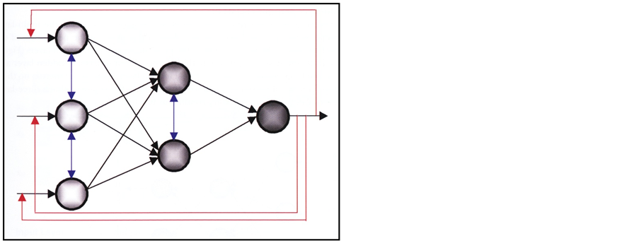
Artificial neural networks are a set of a relatively large number of processing elements (artificial neuron) that are designed in a specific and regular manner and the signals exchange between neurons on the communicational links [10] . Artificial neurons are similar to biological neurons of the human brain. They are parallel processing systems that are used to detect very complex patterns among data and have learning, training and remembering ability and capability of generalizing the results [11] . In this study, initially the available data were processed and inappropriate data were omitted, since they have a negative effect on network training and testing. Then, the data were normalized in (0, 1) interval. The best case for neuron networks is when all inputs and outputs are between 0 and 1. Hence, we normalized the input data (well logging data) and output data (DSI data) in (0, 1) interval to perform the network training in the best possible way. Among all processed data (data from wells No. 1, 2 and 3), data from well No. 1 and well No. 2 were selected as the training set and test and validation set, respectively. Then, a three-layer feed forward neural network (Figure 12) was used to build the model. The network components include neurons and layers. Neurons are organized in layers and each layer is responsible for a specific task. Input layer receives information from the environment and transfers it to the middle layer. Middle layer (hidden) analyses the information entered from the environment into the neural network. Output layer receives the result of analyzed information from middle layer and converts them to a meaningful form and returns them into the environment.
We used try and error method to determine the number of neurons in the middle layer. Accordingly, the best selected network with the highest correlation coefficient and the lowest error has 8 neurons in its hidden layer. Moreover, transfer function from input layer to middle layer is nonlinear tangent sigmoid function (Tansig) and transfer function from the middle layer to the output layer is Purlin linear function.
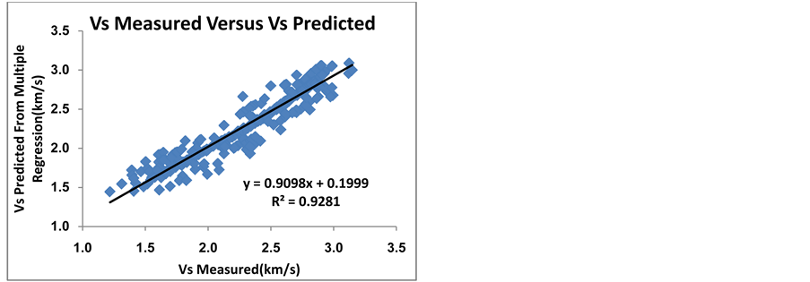
Figure 10. Correlation between measured shear wave velocity and shear wave velocity estimated by multiple regression analysis.
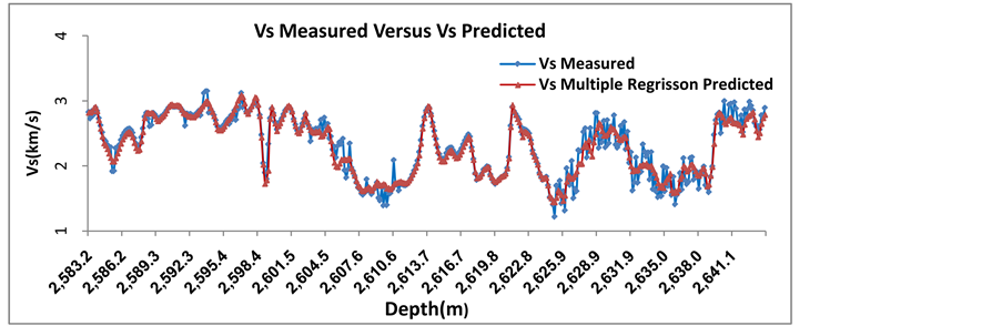
Figure 11. Correlation between measured VS and shear wave velocity estimated by multiple regression versus depth.
We used different training algorithms and transfer functions to design a desirable network. Experimentally, it was proved that feed forward networks with error back-propagation algorithm to determine the geomechanical parameters give the best result. Therefore, in order to estimate shear wave velocity, we used error back-propagation algorithm (which is a feed forward supervised learning algorithm) with Train LM training function. To avoid excessive network training, a particular set named “validation set” was used. Network validation is performed simultaneously with network training in each course and when validation data error begins to rise, the training is stopped. Mean square error (MSE) curve in terms of the number of training course (Epochs) for training data shows that the network has arrived to the best learning and the lowest error after 198 rounds (Figure 13).
In this study, different input sets with various middle neurons were used to predict . Inputs with the smallest error and the highest correlation coefficient were selected as desirable inputs, and finally the best result was belong to a network with five input parameters
  and 8 neurons in the middle layer and the values of correlation coefficients for training and testing stages was about
  and
and , respectively (Figure 14 & Figure 15). Also Figure 16 shows the
  calculated from multiple regression and
  obtained from DSI tool versus the depth. The results demonstrate the high ability of neural networks in predicting geomechanical parameters.
According to the above results, the efficiency of artificial neural network in estimating shear wave velocity is very high. Thus, the  measured by DSI tool and
  calculated from neural network are very close and therefore the results of this network could be generalized to the well No. 3, which hasn’t shear wave velocity.
5. Conclusions
Among the various methods which were presented to estimate the shear wave velocity in the Asmari reservoir,
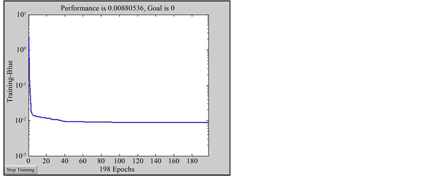
Figure 13. Number of iterations (epochs) versus mean square error (MSE).
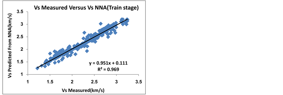
Figure 14. Cross-plot between measured Vs and Vs estimated by neural networks in training stage.
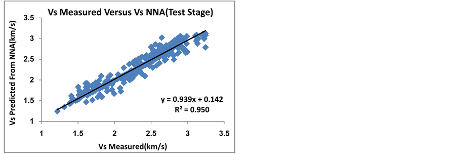
Figure 15. Cross-plot between measured Vs and Vs estimated by neural networks in testing stage.
artificial neural networks were very powerful in estimating shear wave velocity. Neural networks are able to understand the complex causal relationship between shear wave velocity and petrophysical parameters, thus in the case of heterogenic of the reservoir and lack of well logging data, they can provide acceptable results. The results of current study show that there is a good agreement between shear wave velocity obtained from DSI tool, and shear wave velocity estimated from designed neural network. Therefore, network designed in this study is able to acceptably estimate  in other wells of the field, whose data of dipole tool isn’t available for them.
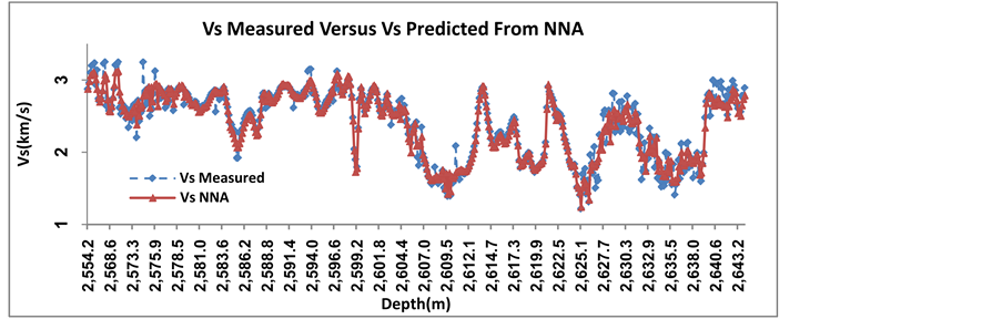
Figure 16. Comparison of measured Vs and Vs estimated by neural network versus depth.
Empirical relationships are used to estimate shear wave velocity which are defined based on different lithologies and a few number of petrophysical parameters such as porosity and compressional wave velocity. In the current study, Castagna relation was used to estimate the . This relation has an input parameter (
 ), and correlation coefficient between shear wave velocity values measured from DSI tool, and obtained with this relation was about 72% (R2 = 0.72). This recommended to use of Castigna’s relation in carbonate reservoirs, when a complete series of well logging data isn’t available, and its results is somewhat acceptable.
In multiple linear regression analysis, input parameters of the model was increased and the effects of different petrophysical parameters such as RHOB, NPHI and  were used to estimate shear wave velocity, and shear wave velocity was predicted with correlation coefficient of 92%. Hence, this method has been successful in estimating
  and has a high importance. However, these methods have some weaknesses that make their applications difficult in some cases. For example, these methods haven’t generalization capability for different lithologies.
References
- Wong, P.M. and Nikravesh, M. (2001) Field Applications of Intelligent Computing Techniques. Journal of Petroleum Geology, 24, 381-387. http://dx.doi.org/10.1111/j.1747-5457.2001.tb00681.x
- Eskandari, H., Rezaee, M.R. and Mohammadnia, M. (2004) Application of Multiple Regression and Artificial Neural Network Techniques to Predict Shear Wave Velocity from Well Log Data for a Carbonate Reservoir, South-West Iran. Cseg Recorder, 42-48.
- Lim, J.S. (2005) Reservoir Properties Determination Using Fuzzy Logic and Neural Networks from Well Data in Offshore Korea. Journal of Petroleum Science and Engineering, 49, 182-192. http://dx.doi.org/10.1016/j.petrol.2005.05.005
- Rezaee, M.R. and Chehrazi, A. (2006) Basics of Acquisition and Interpretation of Wireline Logs. 1st Edition, University of Tehran Press, Tehran.
- Moatazedian, I., Rahimpour-Bonab, H., Kadkhodaie-Ilkhchi, A. and Rajoli, M.R. (2011) Prediction of Shear and Compressional Wave Velocities from Petrophysical Data Utilizing Genetic Algorithms Technique: A Case Study in Hendijan and Abuzar Fields Located in Persian Gulf. Geopersia, 1, 1-17.
- Schlumberger (1989) Log Interpretation: Principles/Applications. Schlumberger Wireline and Testing. 225 Schlumberger Drive, Sugar Land, Texas No. 77478.
- Castagna, J.P., Batzle, M.L. and Eastwood, R.L. (1985) Relationship between Compressional and Shear Wave Velocities in Silicate Rocks. Geophysics, 50, 571-581. http://dx.doi.org/10.1190/1.1441933
- Wang, Z. (2000) Velocity Relationships in Granular Rocks. In: Wang, Z. and Nur, A., Eds., Seismic and Acoustic Velocities in Reservoir Rocks, 3, 145-158.
- Hasanipak, A.A. and Sharafodin, M. (2000) Analyze of Exploration Data. Tehran University Press, Tehran.
- Balan, B., Mohaghegh, S. and Ameri, S. (1995) State-of-Art in Permeability Determination from Well Log Data. Part 1—A Comprehensive Study, Model Development, SPE 30978.
- Bhatt, A. and Hell, H.B. (2002) Committee Neural Networks for Porosity and Permeability Prediction from Well Logs. Geophysical Prospecting, 50, 645-660. http://dx.doi.org/10.1046/j.1365-2478.2002.00346.x
- Aminzade, F. and de Groot, P. (2006) Neural Networks and Other Soft Computing Techniques with Application in the Oil Industry. EAGE Publications, 129.