Open Journal of Discrete Mathematics
Vol.1 No.1(2011), Article ID:4578,16 pages DOI:10.4236/ojdm.2011.11002
Solution of Stochastic Cubic and Quintic Nonlinear Diffusion Equation Using WHEP, Pickard and HPM Methods
1Cairo university, Faculty of Engineering, Engineering, Mathematics Department, Giza, Egypt
2Benha university, Benha Higher Institute of Technology, Basic Science Department, Benha, Egypt
E-mail: {magdyeltawil, aisha.farid}@yahoo.com
Received March 13, 2011; revised March 23, 2011; accepted April 3, 2011
Keywords: Stochastic diffusion equations, WHEP technique, HPM method
Abstract
In this paper, the cubic and quintic diffusion equation under stochastic non homogeneity is solved using WienerHermite expansion and perturbation (WHEP) technique, Homotopy perturbation method (HPM) and Pickard approximation technique. The analytic solution of the linear case is obtained using Eigenfunction expansion .The Picard approximation method is used to introduce the first and second order approximate solution for the non linear case. The WHEP technique is also used to obtain approximate solution under different orders and different corrections. The Homotopy perturbation method (HPM) is also used to obtain some approximation orders for mean and variance. Using mathematica-5, the methods of solution are illustrated through figures, comparisons among different methods and some parametric studies.
1. Introduction
The study of random solutions of partial differential equations was initiated by Kampe de Feriet in 1955 [1]. In his valuable survey on the theory of random equations, Bharucha-Reid showed how a stochastic heat equation of Cauchy type can be solved using the stochastic integrals theory[2]. In 1973, Lo Dato V. [3] considered the stochastic velocity field and the Navier-Stokes equation and discussed the mathematical problems associated with it. Becus A. Georges [4] introduced a general solution for the heat conduction problem with a random source term and random initial and boundary conditions. Many authors investigated the stochastic diffusion equation under different views, see [5-11].
El-Tawil M. used the Wiener-Hermite expansion together with perturbation theory (WHEP technique) to solve a perturbed nonlinear stochastic diffusion equation [12]. The technique has been then developed to be applied on non-perturbed differential equations using the homotopy perturbation method and is called Homotopy WHEP [13,14]. El-Tawil M. and Noha A. El-Molla.[15] solved the quadratic and cubic non-linear stochastic diffusion equation using Pickard approximation and homotopy WHEP technique [16].
The diffusion equation with cubic and quintic nonlinear losses and stochastic non homogeneity are solved using different techniques, mainly the Pickard approximation, the WHEP technique and HPM. The main goal of the paper is to compare among these different techniques. Some statistical moments are obtained, mainly the ensemble average, covariance and variance of the solution processes. In Sections 2.1 and 3.1, the Pickard approximation technique is used in solving the cubic and quintic nonlinear diffusion problems respectively. WHEP technique is processed in Sections 2.2 and 3.2, while HPM is used in Sections 2. 3 and 3. 3. Some comparisons are illustrated in different sections.
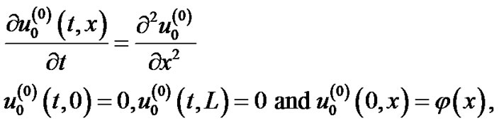
2. The Cubic Nonlinear Stochastic Diffusion Equation
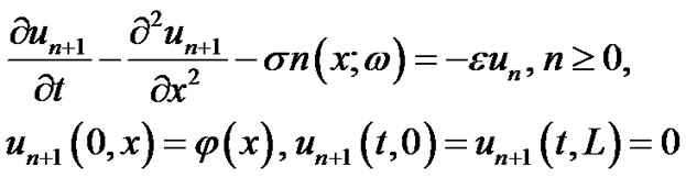
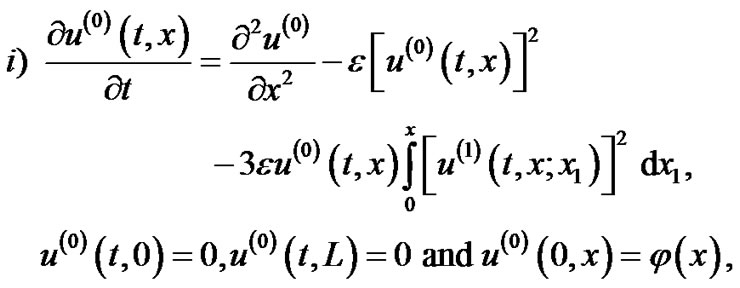
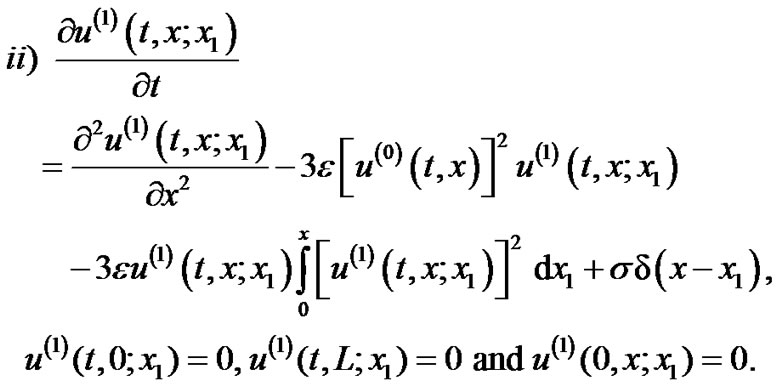
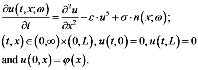
Let us consider the following stochastic nonlinear-diffusion equation with cubic nonlinear losses, :
:
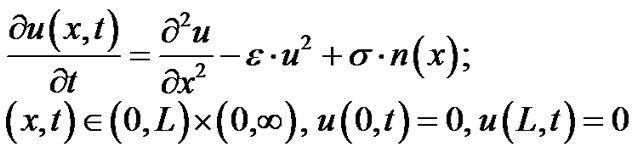
 (1)
(1)
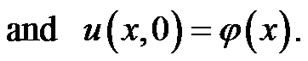
Where ![]() is a deterministic scale for the nonlinear term. The in homogeneity term
is a deterministic scale for the nonlinear term. The in homogeneity term 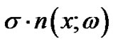 is space white noise scaled by
![]() .
.
Three methods are used in the next subsections, mainly the Pickard approximations, the WHEP technique and Homotopy perturbation method.
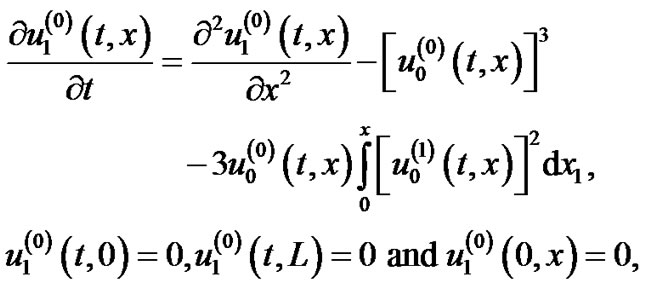
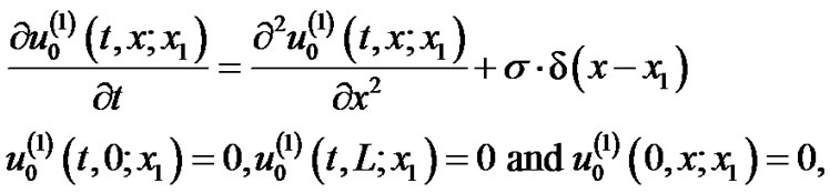
2.1. Using Pickard Approximation
In this technique, the linear part of the differential operator is kept in the left hand side of the equation whereas the rest of the nonlinear terms are moved to the right part. The successive Pickard approximations are processed according to letting the L.H.S. as the  approximation for the solution process depending on the
  approximation in the R.H.S,
  Following this routine and applying it on to (1), we get the following iterative equations:
 (2)
(2)
 (3)
(3)
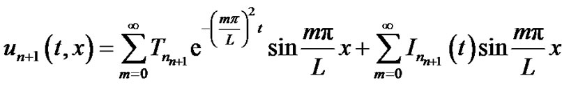
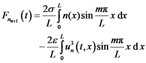
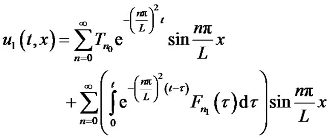
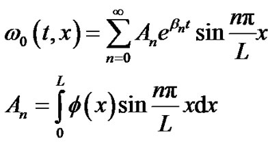
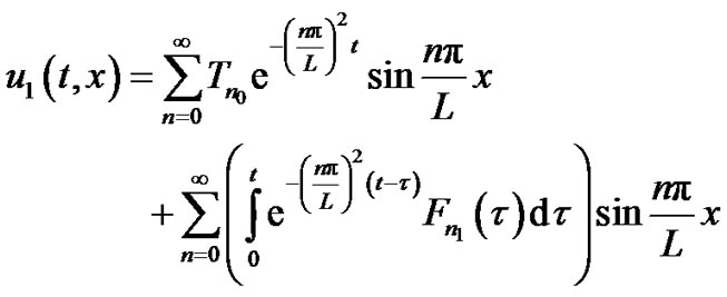
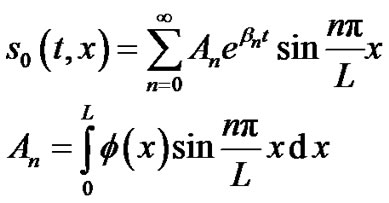
Using Eigen function expansion, the following general solutions are got
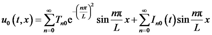 (4)
(4)
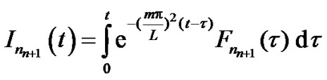
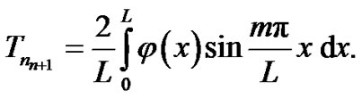
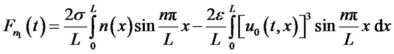
where
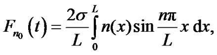 (5)
(5)
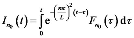 (6)
(6)
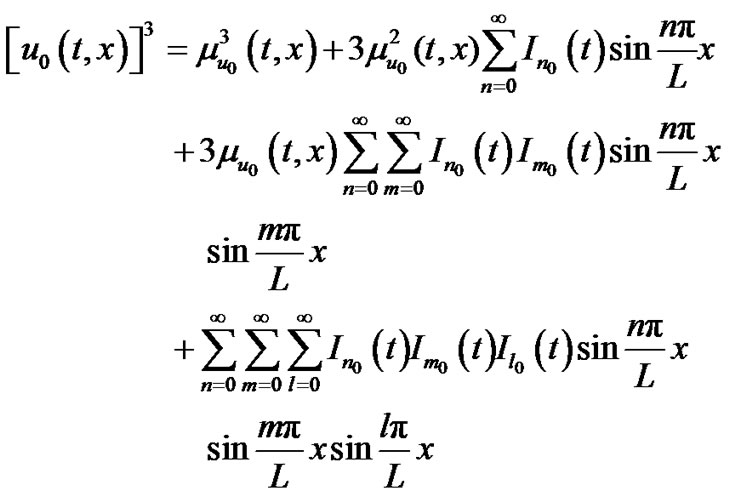
Also,
where
 (8)
(8)
 (9)
(9)
 (10)
(10)
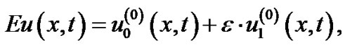
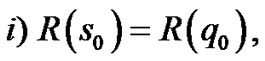
If the convergence of the process is insured, one can obtain the solution as
![]() (11)
(11)
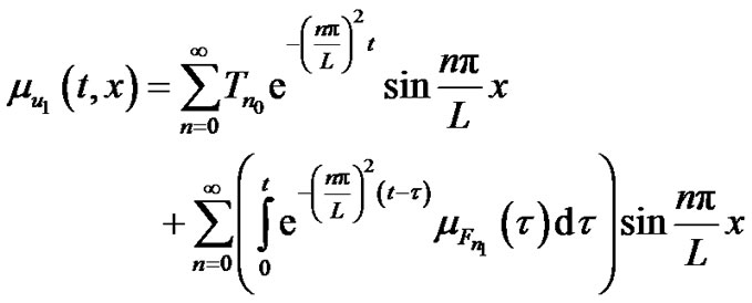
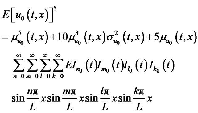
One can notice that all order of approximations are stochastic processes. The ensemble average of the zero order approximation is obtained as
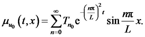 (12)
(12)
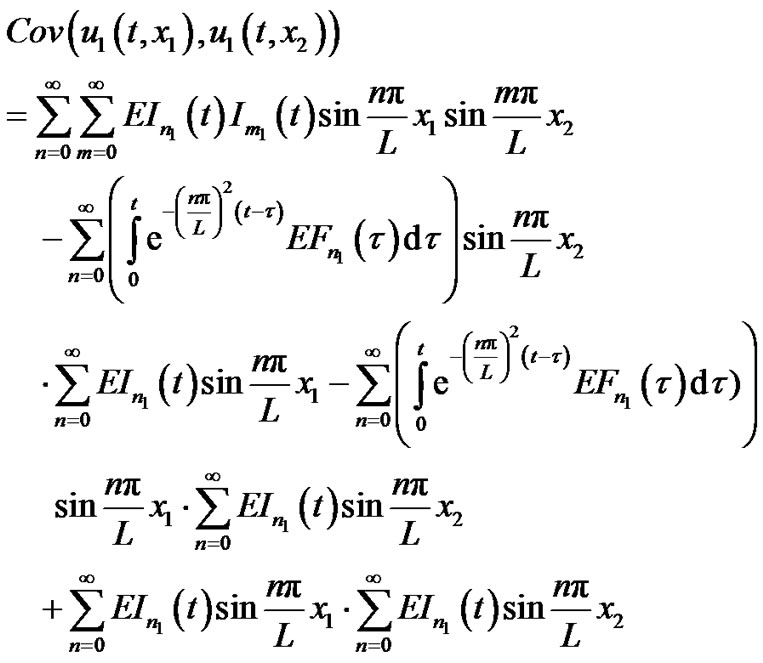
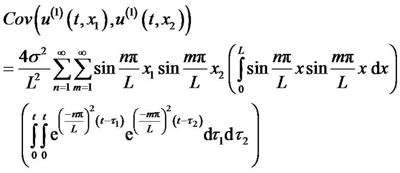
The covariance of  is given by
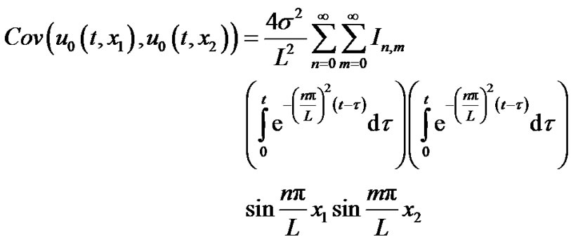
(13)
where
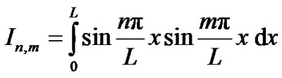 (14)
(14)
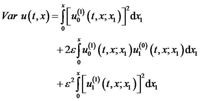
The variance is
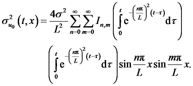 (15)
(15)
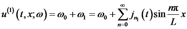
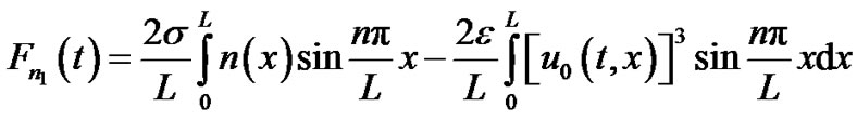
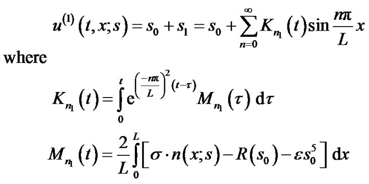
The following results for the first order approximation are obtained:
 (16)
(16)
where
 (18)
(18)
 (19)
(19)
where
 (20)
(20)
 (21)
(21)
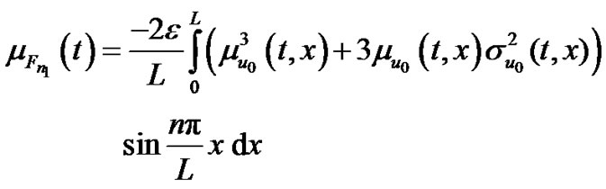
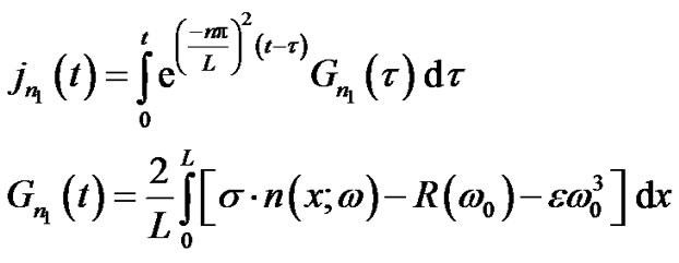
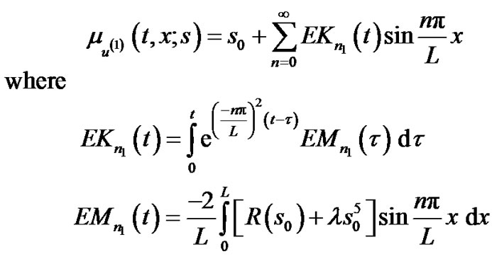
where E denotes the ensemble average operator and
 (22)
(22)
 (23)
(23)
In which
where
In which
 (26)
(26)
 (27)
(27)
And
In which
 (29)
(29)
 (30)
(30)
 (31)
(31)
 (32)
(32)
 (34)
(34)
 (35)
(35)
 (36)
(36)
where
Using mathematica-5, the previous huge computations were performed and the following sample results are obtained:
Figures 1 and 2 illustrates the change of the first order mean and variance under the change of some illustrated parameters.
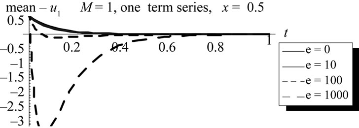
Figure 1. The change of the mean of first order approximation u1 with time t at x = 0.1 with different ε values, (L = 1, M = 1, σ = 1, Φ(x) = x).
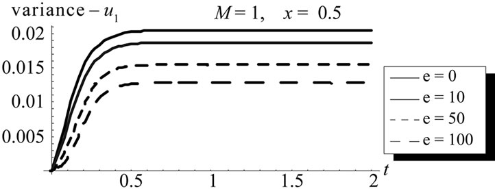
Figure 2. The change of the variance of the first order approximation u1 with time t and space variable x at x = 0.5 at different ε values, (L = 1, M = 1, σ = 1, Φ(x) = x).
One can notice that the mean diminishes with time for all ε while the variance decreases with the increase of ε.
Following similar computation procedure, the following results for the second order approximations of the mean is illustrated in figures 3, 4, 5 and 6.
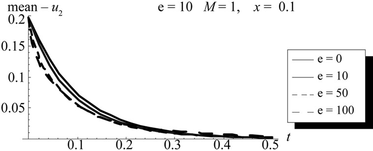
Figure 3. The change of the mean of second order approximation u2 with time t at x = 0.1 with different ε values, (L = 1, M = 1, σ = 1, Φ(x) = x).
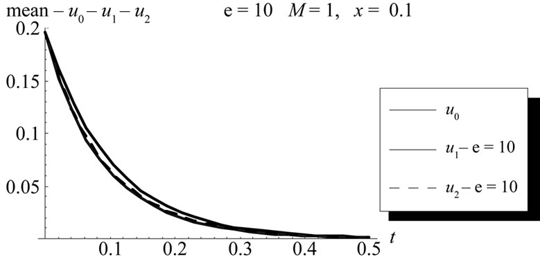
Figure 4. The change of the mean of zero, first and second order approximation (u0, u1, u2) with time t at x = 0.1, ε = 10, (L = 1, M = 1, σ = 1, Φ(x) = x).
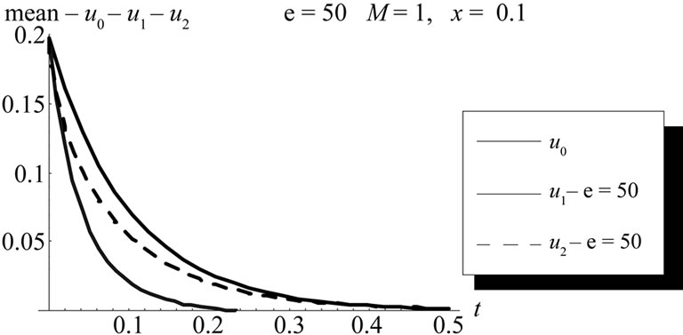
Figure 5. The change of the mean of zero, first and second order approximation (u0, u1, u2) with time t at x = 0.1, ε = 50, (L = 1, M = 1, σ = 1, Φ(x) = x).
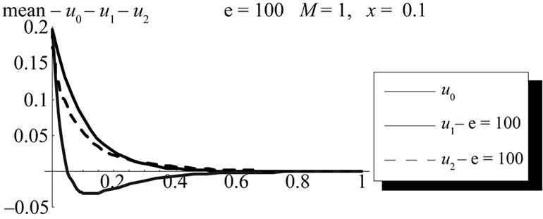
Figure 6. The change of the mean of zero, first and second order approximation (u0, u1, u2) with time t at x = 0.1, ε = 100, (L = 1, M = 1, σ = 1, Φ(x) = x).
2.2. Using WHEP Technique
Since Meecham and his co-workers [25] developed a theory of turbulence involving a truncated Wiener-Hermite expansion (WHE) of the velocity field, many authors studied problems concerning turbulence [26-27]. A lot of general applications in fluid mechanics was also studied in [28]. Scattering problems attracted the WHE applications through many authors [29]. The nonlinear oscillators were considered as an opened area for the applications of WHE as can be found in [30]. There are a lot of applications in boundary value problems [31] and generally in different mathematical studies [32].
The application of the WHE aims at finding a truncated series solution to the solution process of differential equations. The truncated series composes of two major parts; the first is the Gaussian part which consists of the first two terms, while the rest of the series constitute the non-Gaussian part. In nonlinear cases, there exist always difficulties of solving the resultant set of deterministic integro-differential equations got from the applications of a set of comprehensive averages on the stochastic integro-differential equation obtained after the direct application of WHE. Many authors introduced different methods to face these obstacles. Among them, the WHEP technique was introduced in [33] using the perturbation technique to solve perturbed nonlinear problems.
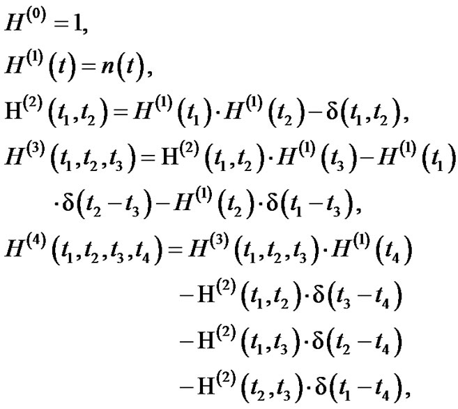
The WHE method utilizes the Wiener-Hermite polynomials which are the elements of a complete set of statistically orthogonal random functions [34]. The WienerHermite polynomial 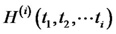 satisfies the following recurrence relation:
 (38)
(38)
where
 (39)
(39)
In which n(t) is the white noise as noted with the following statistical properties
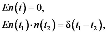 (40)
(40)
Where δ (-) is the Dirac delta function and. The Wiener-Hermite set is a statistically orthogonal set, i.e.
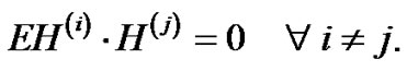 (41)
(41)
The average of almost all H functions vanishes, particularly,
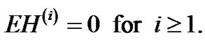 (42)
(42)
Due to the completeness of the Wiener-Hermite set, any random function  can be expanded as
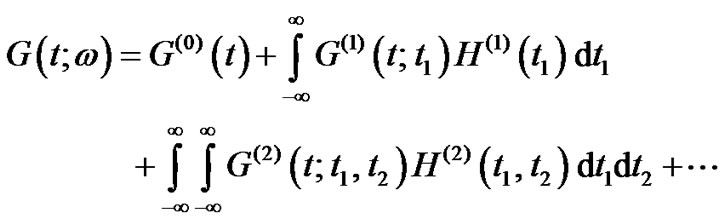 (43)
(43)
Where the first two terms are the Gaussian part of .The rest of the terms in the expansion represent the non-Gaussian part of
 . The average of
  is:
is:
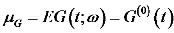 (44)
(44)
The covariance of  is
is
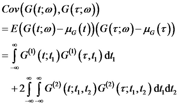 (45)
(45)
The variance of  is
is
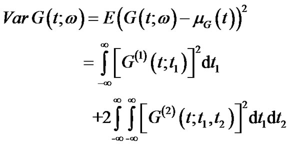 (46)
(46)
The WHEP technique can be applied on linear or nonlinear perturbed systems described by ordinary or partial differential equations. The solution can be modified in the sense that additional parts of the WienerHermite expansion can always be taken into considerations and the required order of approximations can always be made depending on the computing tool. It can be even run through a package if it is coded in some sort of symbolic languages. The technique was successfully applied to several nonlinear stochastic equations, see [20-25].
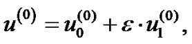
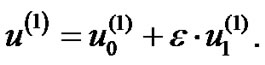
The first order solution can be obtained when considering only the Gaussian part of the solution process, i.e  can be expanded as:
 (47)
(47)
Substituting in the original equation (1) and taking the necessary averages, we get the following two sets of deterministic equations:
 (48)
(48)
Applying WHEP technique, the deterministic kernels can be represented in first order approximation as:
 (50)
(50)
 (51)
(51)
Substituting in the previous set of equations (48) and (49), we get the following four sets of equations:
 (52)
(52)
 (53)
(53)
 (54)
(54)
 (55)
(55)
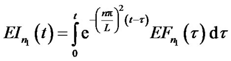
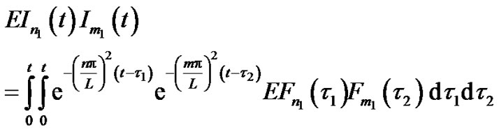
The algorithm of solution is evaluating  and
and  first using the separation of variables and the Eigen function expansion respectively and then computing the other two kernels independently using the Eigenfunction expansion. The final results are:
 (56)
(56)
 (57)
(57)
The result can be made better using the second correction as the following formula:
 (58)
(58)
 (59)
(59)
The following are some sample results.
2.2.1. First Order Approximation and Different Corrections Results
Figures 7 and 8 illustrate the change of the first order mean and variance under different correction levels.
We can notice the stable results for the different corrections.
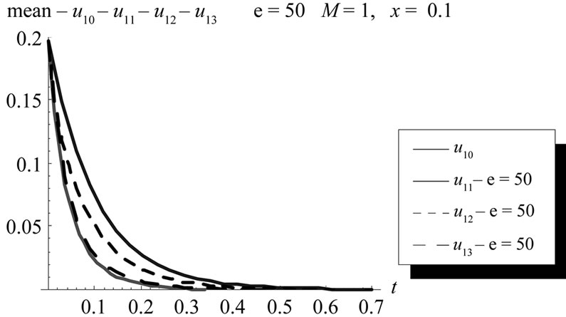
Figure 7. Mean comparison between first order with zero, first, second and third corrections at ε = 50 at x = 0.1, (L = 1, M = 1, σ = 1, Φ(x) = x).
2.2.2. Second Order Approximation and Different Corrections Results
Figures 9 and 10 illustrate the change of the second order mean and variance under different correction levels.
2.2.3. Mean and Variance Comparisons between First and Second Order Approximations with Different Corrections Results
Figures 11 and 12 illustrate in a comparative way, the mean and variance under first and second orders with some correction levels.
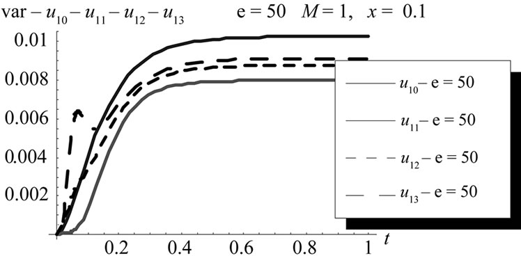
Figure 8. Variance comparison between first order with zero, first, second and third corrections at x = 0.1 at ε = 50, (L = 1, M = 1, σ = 1, Φ(x) = x).
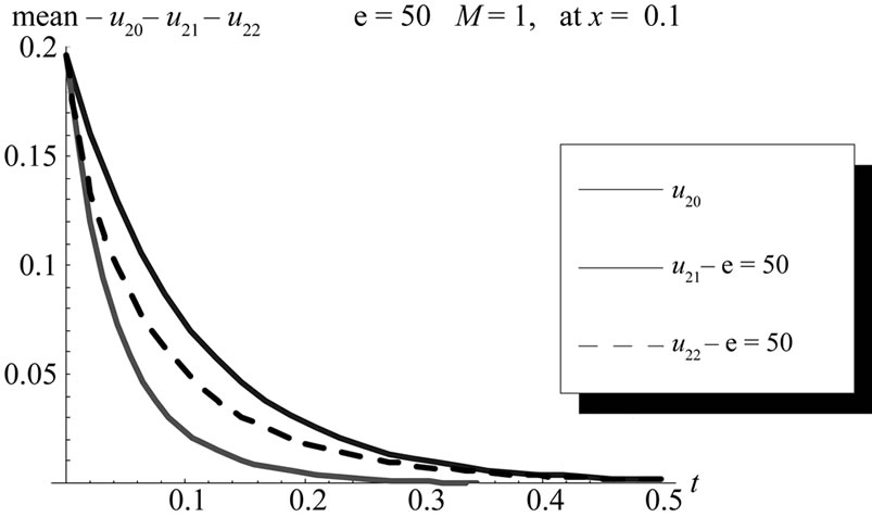
Figure 9. Mean comparison between second order with zero, first and second corrections at x = 0.1, ε = 50, (L = 1, M = 1, σ = 1, Φ(x) = x).
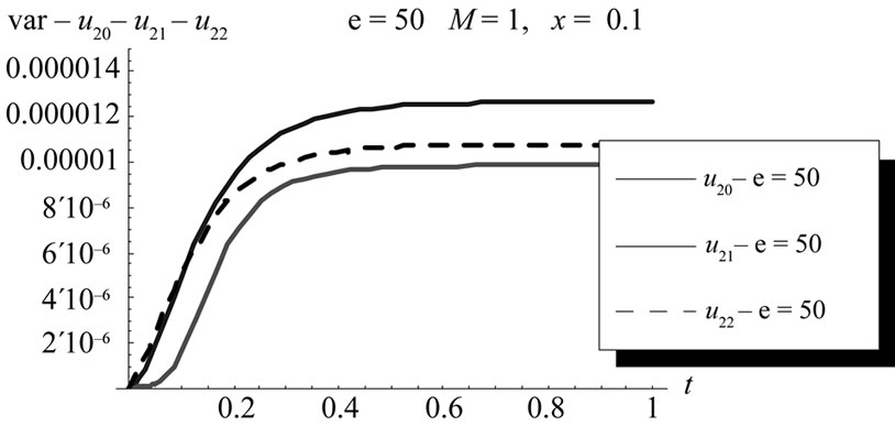
Figure 10. Variance comparison between second order with zero, first and second corrections at x = 0.1, ε = 50, (L = 1, M = 1, σ = 1, Φ(x) = x).
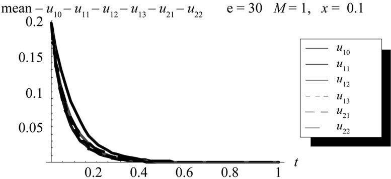
Figure 11. Mean comparison between first order with zero, first, second and third corrections, second order with first and second corrections at x = 0.1 at ε = 30, (L = 1, M = 1, σ = 1, Φ(x) = x).
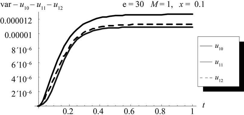
Figure 12. Variance comparison between first order with zero, first and second corrections at x = 0.1 at ε = 30 (L = 1, M = 1, σ = 1, Φ(x) = x).
2.3. Using Homotopy Perturbation Technique (HPM)
In homotopy Perturbation method (HPM) [18-21], a parameter  is embedded in a homotopy function
  which satisfies
 (60)
(60)
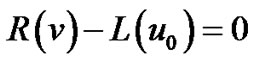
Where  is an initial approximation to the solution of the equation:
 (61)
(61)
With boundary condition
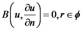 (62)
(62)
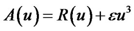
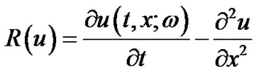
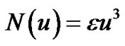
In which A is a nonlinear differential operator which can be decomposed into a linear operator R and anon linear operator N,B is a boundary operator, f(r) is a known analytic function and Г is the boundary of Φ .the homotopy introduces a continuously deformed solution for the case ,
,  , which is the original equation .this is the basic idea of the homotopy method which is to deform continuously a simple problem (and easy to solve)into the difficult problem under study.
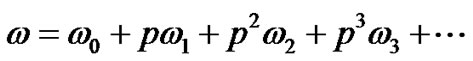
The basic assumption of the (HPM) method is that the solution of the original equation can be expanded as a power series in p as:
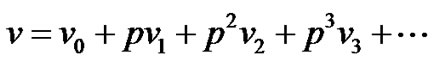 (63)
(63)
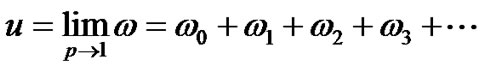
Now, setting p = 1, the approximation solution is obtained as:
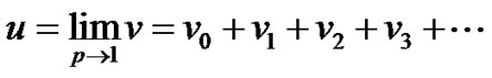 (64)
(64)
The rate of convergence of the method depends greatly on the initial approximation  which is considered as the main disadvantage of HPM. The idea of imbedded parameter can be utilized to solve nonlinear problems by imbedding this parameter to the problem and then forcing it to be unity in the obtained approximate solution if convergence can be assured .it is a simple technique which enables the extension of the applicability of the perturbation method from small value applications to general ones.
Applying HPM on equation (1), we can get the following results w. r. t homotopy perturbation:
 (65)
(65)
 (66)
(66)
 (67)
(67)
 (68)
(68)
The homotopy function takes the following form:
 (69)
(69)
Or equivalently,
 (70)
(70)
Where z0 is an initial solution .The approximate solution can then be obtained using
 (71)
(71)
Now, setting p = 1, the approximation solution is obtained as:
 (72)
(72)
Using equation (86) in equation (85) and equating the equal powers of p in both sides of the equation, one can get the following results:
 in which one may consider the following simple solution:

 (73)
(73)
 (74)
(74)
 (75)
(75)
 (76)
(76)
 (77)
(77)
As before we have many choices in guessing the initial approximation together with its initial conditions which greatly affects the consequent approximation .the choice  is a design problem which can be taken as follows:
 (78)
(78)
One can notice that the selected value function satisfies the initial and boundary conditions and it depends on the parameter βn which is totally free .One can also notice that βn selection could control the solution convergence.
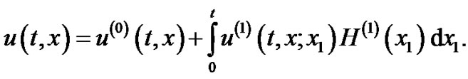
The first order approximation can be obtained using Eigen function expansion as follows:
where
 (79)
(79)
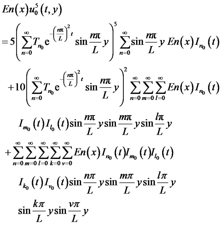
The ensemble average is
 (80)
(80)
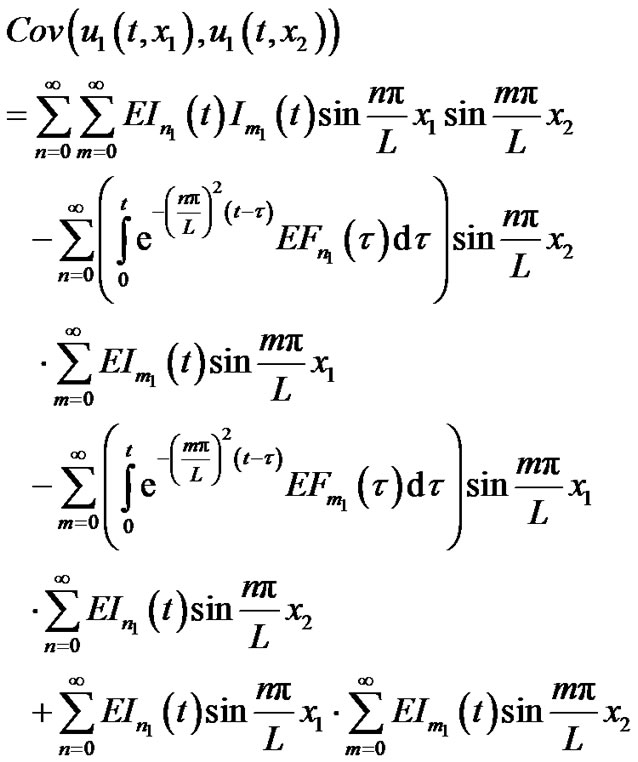
The covariance is obtained from the following final expression
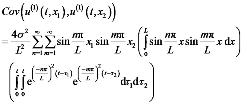
The variance can then be obtained from equation (81) by setting x1 = x2 = x.
Any higher order approximations can be obtained in a similar way. The following sample results using the same data in the cubic case.
Computing the consequent errors  by using the following expression
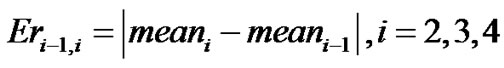 (82)
(82)
we obtain the following results. Figures 13 illustrates different mean approximations using homotopy method (HPM) with computing their corresponding decreasing errors in figure 14.
Figures 15 illustrates different variance approximations using homotopy method (HPM) with computing their corresponding decreasing errors in figure 16.
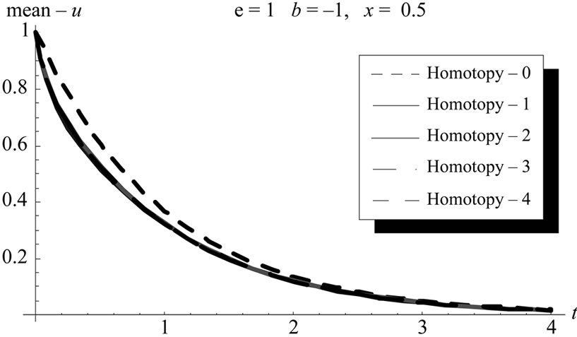
Figure 13. The mean at different homotopy orders, cubic case.
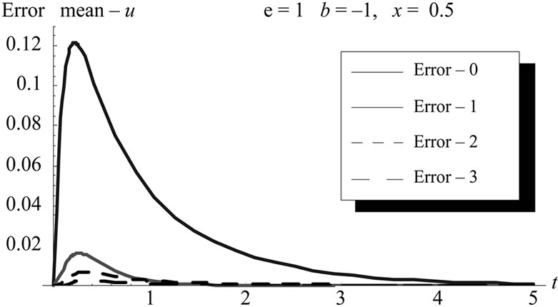
Figure 14. The error differences, cubic case.
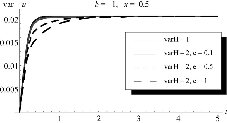
Figure 15. The variance (-1: first and-2: second) at different ε, HPM, cubic nonlinear case.
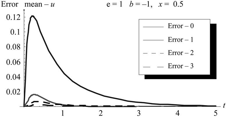
Figure 16. The error difference of first and second error at different ε, cubic case.
2.4. Mean and Variance Comparisons of the Solution of Stochastic Cubic Nonlinear Diffusion Problem Using WHEP, Pickard and HPM Methods with Different Orders and Corrections
Figures 17, 18, 19 and 20 illustrate some useful comparisons among the three used methods in this paper.
3. The Quintic Nonlinear Stochastic Diffusion Equation
Let us consider the following stochastic nonlinear-diffusion equation
 (83)
(83)
Where ε is a deterministic scale for the nonlinear term. Two methods are used in the next subsections, mainly the Pickard approximations and the HPM technique.
3.1. Using the Pickard Approximation
The following results for the first order approximation are obtained
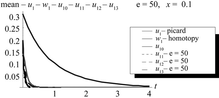
Figure 17. Mean comparison between Picard first order, Homotopy first order and WHEP first order with zero, first, second and third corrections at x = 0.1, ε = 50, (L = 1, M = 1, σ = 1, Φ(x) = x).
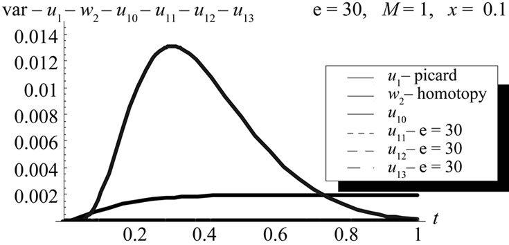
Figure 18. Variance comparison between Picard first order, Homotopy second order and WHEP first order with zero, first, second and third corrections at x = 0.1, ε = 30, (L = 1, M = 1, σ = 1, Φ(x) = x).
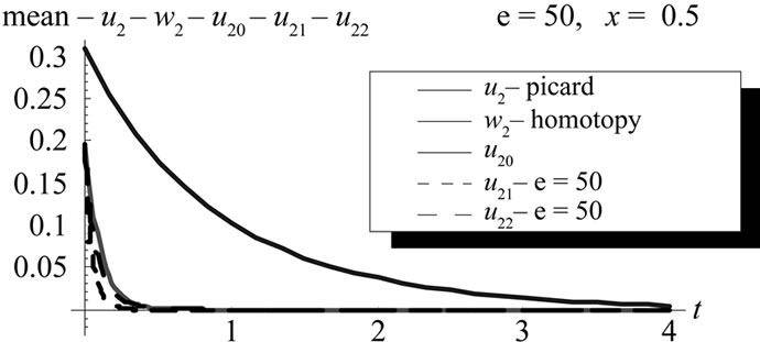
Figure 19. Mean comparison between Picard second order , Homotopy fourth order and WHEP second order with zero, first, second and third corrections at x = 0.5 , ε = 50, (L = 1, M = 1, σ = 1, Φ(x) = x).
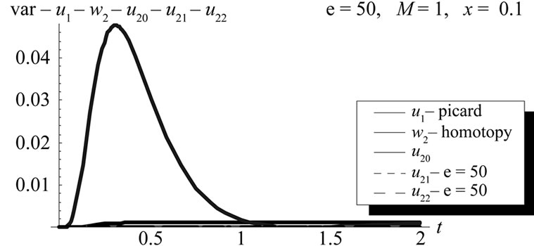
Figure 20. Variance comparison between Picard first order, Homotopy second order and WHEP second order with zero, first and second corrections at x = 0.1, ε = 50, (L = 1, M = 1, σ = 1, Φ(x) = x).
 (84)
(84)
where
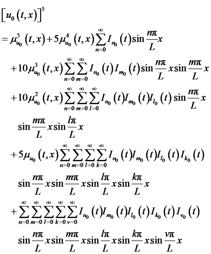 (86)
(86)
First order mean
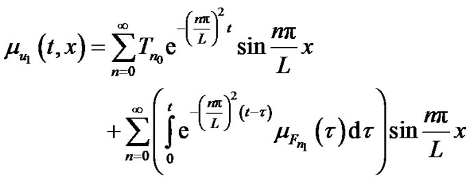 (87)
(87)
where
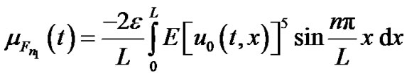 (88)
(88)
 (89)
(89)
where
 (91)
(91)
In which
 (93)
(93)
 (94)
(94)
 (95)
(95)
Figures 21 and 22 illustrate the change of the mean and variance under the nonlinear scale parameter.
3.2. Using HPM Technique
Applying HPM on equation (38), one can get the following results w. r. t homotopy perturbation:
 (96)
(96)
 (97)
(97)
 (98)
(98)
 (99)
(99)
The homotopy function takes the following form:
 (100)
(100)
Or equivalently,
 (101)
(101)
Where z0 is an initial solution .The approximate solution can then be obtained using
 (102)
(102)
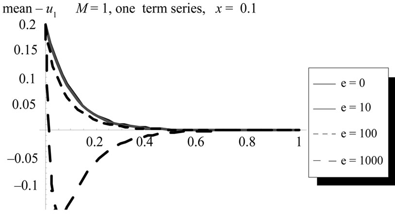
Figure 21. The change of the mean of the first order approximation u1 with time t at x = 0.1 For different ε values, (L = 1, M = 1, σ = 1, Φ(x) = x).
Now, setting p = 1, the approximation solution is obtained as:
 (103)
(103)
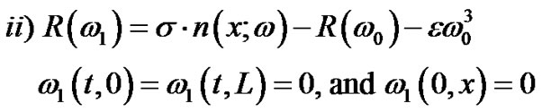
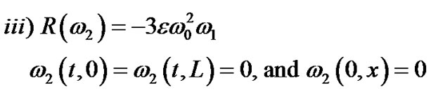
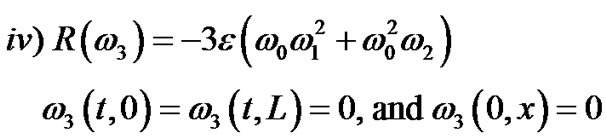
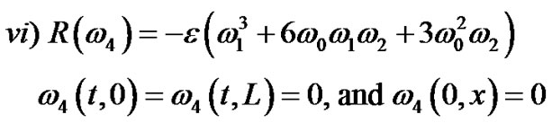
Using equation (102) in equation (101) and equating the equal powers of p in both sides of the equation, one can get the following results:
 in which one may consider the following simple solution:
 (104)
(104)
 (105)
(105)
 (106)
(106)
 (107)
(107)
 (108)
(108)
As before we have many choices in guessing the initial approximation together with its initial conditions which
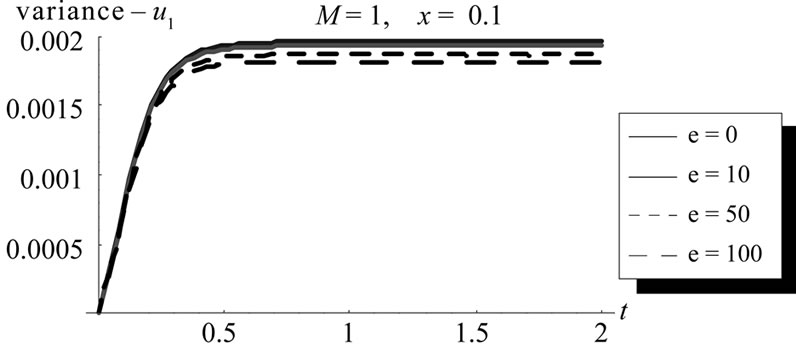
Figure 22. The change of the variance of the first order approximation u1 with time t and space variable x at different ε values, (L = 1, M = 1, σ = 1, Φ(x) = x).
greatly affects the consequent approximation. the choice  is a design problem which can be taken as follows:
 (109)
(109)
First order approximation can be obtained using Eigenfunction expansion as follows:
 (110)
(110)
The ensemble average is:
 (111)
(111)
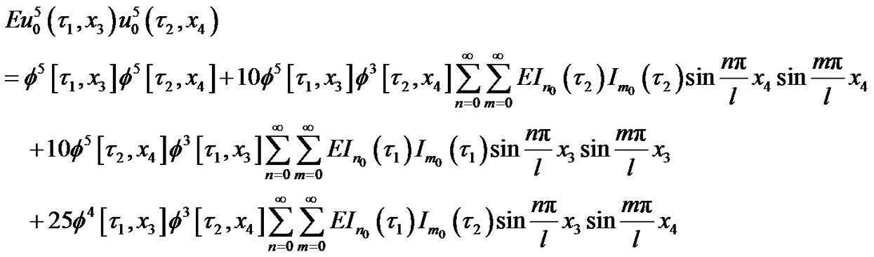
The covariance is obtained from the following final expression
(112)
The variance can then be obtained from equation (112) by setting x1 = x2 = x.
Any higher order approximations can be obtained in a similar way. The following sample results using the same data in the cubic case.
3.3. Mean and Variance Comparisons of the Solution of Stochastic Quintic Nonlinear Diffusion Problem Using Pickard and HPM Methods with Different Orders and Corrections
Figures 23, 24 and 25 illustrate the change of the mean and variance for Picard and HPM approximations.
4. Conclousion
Comparisons among results of the computations of mean illustrates that the results of three methods are very close from each other, but in variance the results of HPM and WHEP are semi-simillar while some results of Pickard are different in magnitude, may be due to the inability of computing high order approximations. It seems that the WHEP technique is more complex, in computations sense, than HPM which is more general since it can be
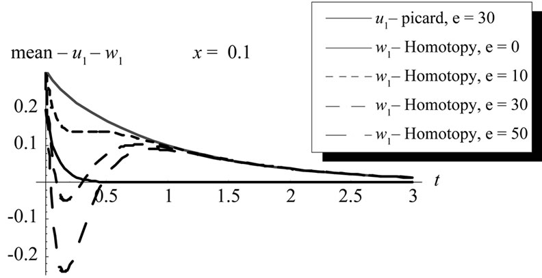
Figure 23. Mean comparison between Picard first order at ε = 30 and HPM first order at different ε values, (u1, w1) at x = 0.1, (L = 1, M = 1, σ = 1, Φ(x) = x).
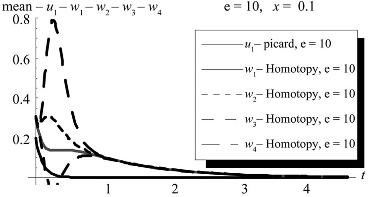
Figure 24. Mean comparison between Picard first order and HPM first, second, third and fourth order at ε = 10, (u1, w1, w2, w3, w4) at x = 0.1, (L = 1, M = 1, σ = 1, Φ(x) = x).
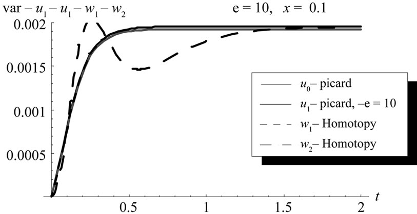
Figure 25. Variance comparison between Picard zero and first order, HPM first and second order, (u0, u1, w1, w2) at x = 0.1, ε = 10, (L = 1, M = 1, σ = 1, Φ(x) = x).
applied to a non-perturbative problems as well as perturbative ones. The WHEP technique has the advantage of making different corrections for each order of approximation. The HPM seems easier in computations sense but it is very sensitive to initial guess solution. Symbolic computations with higher computations abilities will lead to better approximate solutions in the future.
5. References
[1] Kampe de Feriet: Random solutions of partial differential equations, In: Proc. 3rd Berkeley Symposiumon Mathematical Statistics and Probability–1955, vol. III, pp. 199- 208 (1956).
[2] Bharucha-Reid: A survey on the theory of random functions. The Institute of Mathematical Sciences: Matscience Report 31, India (1965).
[3] Lo Dato, V.: Stochastic processes in heat and mass transport, C. In: Bharucha-Reid (ed.) Probabilistic Methods in Applied Mathematics, vol. 3, pp. 183-212. Academic, New York (1973).
[4] Becus, A. G.: Random generalized solutions to the heat equations. J. Math. Anal. Appl. 60, 93-102 (1977). doi:10.1016/0022-247X(77)90051-8
[5] Marcus, R.: Parabolic Ito equation with monotone nonlinearities. J. Funct. Anal. 29, 257-286 (1978). doi:10.1016/0022-1236(78)90031-9
[6] Manthey, R.: Weak convergence of solutions of the heat equation with Gaussian noise. Math. Nachr. 123, 157-168 (1985). doi:10.1002/mana.19851230115
[7] Manthey, R.: Existence and uniqueness of a solution of a reaction-diffusion with polynomial nonlinearity and with noise disturbance. Math. Nachr. 125, 121-133 (1986).
[8] Jetschke, G.: II. Most probable states of a nonlinear Brownian bridge. Forschungsergebnisse (Jena) N/86/20 (1986).
[9] Jetschke, G.: III. Tunneling in a bistable infinitedimensional potential. Forschungsergebnisse (Jena) N/86/40 (1986).
[10] El-Tawil, M.: Nonhomogeneous boundary value problems. J. Math. Anal. Appl. 200, 53-65 (1996). doi:10.1006/jmaa.1996.0190
[11] Uemura, H.: Construction of the solution of 1-dim heat equation with white noise potential and its asymptotic behaviour. Stoch. Anal. Appl. 14(4), 487-506 (1996). doi:10.1080/07362999608809452
[12] El-Tawil, M.: The application ofWHEP technique on partial differential equations. Int. J. Differ. Equ. Appl. 7(3), 325-337 (2003).
[13] El-Tawil, M.: The homotopy Wiener-Hermite expansion and perturbation technique (WHEP). In: Transactions on Computational Science I. LNCS, vol. 4750, pp. 159-180. Springer, New York (2008). doi:10.1007/978-3-540-79299-4_9
[14] Crow, S., Canavan, G.: Relationship between a WienerHermite expansion and an energy cascade. J. Fluid Mech. 41(2), 387-403 (1970). doi:10.1017/S0022112070000654
[15] El-Tawil M. and Noha A. El-Molla, The approximate solution of a nonlinear diffusion equation using some techniques, a comparison study, International Journal of Nonlinear Sciences and numerical Simulation, 10(3), 687-698, 2009.
[16] El-Tawil M. and Noha A. El-Molla, Solving nonlinear diffusion equations without stochastic homogeneity using the homotopy perturbation method, J. of applied mathematics, pp. 281-299, 2009.
[17] Farlow, S. J.: Partial Differential Equations for Scientists and Engineers. Wiley, New York (1982).
[18] He, J. H.: Homotopy perturbation technique. Comput. Methods Appl. Mech. Eng. 178, 257-292(1999). doi:10.1016/S0045-7825(99)00018-3
[19] He, J. H.: A coupling method of a homotopy technique and a perturbation technique for nonlinear problems. Int. J. Nonlinear Mech. 35, 37-43 (2000). doi:10.1016/S0020-7462(98)00085-7
[20] He, J. H.: Homotopy perturbation method: a new nonlinear analytical technique. Appl.Math. Comput. 135, 73-79 (2003). doi:10.1016/S0096-3003(01)00312-5
[21] He, J. H.: The homotopy perturbation method for nonlinear oscillators with discontinuities. Appl.Math. Comput. 151, 287-292 (2004). doi:10.1016/S0096-3003(03)00341-2
[22] El-Tawil M., International Journal of Differential Equations and its Applications, Vol. 7, No. 3, pp 325-337, 2003.
[23] El-Tawil M., The Homotopy Wiener-Hermite expansion and perturbation technique (WHEP), Transactions on Computational Science (Springer), accepted.
[24] Farlow S. J., Partial differential equations for scientists and engineers, Wiley, N. Y., 1982.
[25] Crow S. and Canavan G., Relationship between a Wiener-Hermite expansion and an energy cascade, J. of fluid mechanics, 41(2), pp. 387-403 (1970). doi:10.1017/S0022112070000654
[26] Saffman P., Application of Wiener-Hermite expansion to the diffusion of a passive scalar in a homogeneous turbulent flow, Physics of fluids, 12(9), pp. 1786-1798(1969). doi:10.1063/1.1692743
[27] Kahan W. and Siegel A., Cameron-Martin-Wiener method in turbulence and in Burger’s model: General formulae and application to late decay, J. of fluid mechanics, 41(3), pp. 593-618 (1970).
[28] Chorin and Alexandre J., Gaussian fields and random flow, J. of fluid of mechanics, 63(1), pp. 21-32(1974).
[29] Eftimiu and Cornel, First-order Wiener-Hermite expansion in the electromagnetic scattering by conducting rough surfaces, Radio science, 23(5), pp. 769-779(1988).
[30] Jahedi A. and Ahmadi G., Application of Wiener-Hermite expansion to non-stationary random vibration of a Duffing oscillator, J. of applied mechanics, Transactions ASME, 50(2), pp. 436-442(1983). doi:10.1115/1.3167056
[31] Tamura Y. and Nakayama J., A formula on the Hermite expansion and its aoolication to a random boundary value problem, IEICE Transactions on electronics, E86-C(8), pp. 1743-1748 (2003).
[32] Kayanuma Y. and Noba K., Wiener-Hermite expansion formalism for the stochastic model of a driven quantum system, Chemical physics, 268(1-3), pp. 177-188(2001). doi:10.1016/S0301-0104(01)00305-6
[33] Gawad E. and El-Tawil M., General stochastic oscillatory systems, Applied Mathematical Modelling, 17(6), pp. 329-335(1993). doi:10.1016/0307-904X(93)90058-O
[34] Imamura T. Meecham W. and Siegel A., Symbolic calculus of the Wiener process and Wiener-Hermite functionals, J. math. Phys., 6(5), pp. 695-706(1983).