American Journal of Computational Mathematics
Vol.2 No.4(2012), Article ID:25492,11 pages DOI:10.4236/ajcm.2012.24035
Optimal Recovery of Holomorphic Functions from Inaccurate Information about Radial Integration
Department of Mathematics and Statistics, State University of New York at Albany, Albany, USA
Email: adegraw@albany.edu
Received April 30, 2012; revised August 20, 2012; accepted September 2, 2012
Keywords: Approximation; Optimal Recovery; Holomorphic
ABSTRACT
This paper addresses the optimal recovery of functions from Hilbert spaces of functions on the unit disc. The estimation, or recovery, is performed from inaccurate information given by integration along radial paths. For a holomorphic function expressed as a series, three distinct situations are considered: where the information error in  norm is bound by
  or for a finite number of terms the error in
  norm is bound by
  or lastly the error in the
  coefficient is bound by
 . The results are applied to the Hardy-Sobolev and Bergman-Sobolev spaces.
1. Introduction
Let W be a subset of a linear space X, let Z be a normed linear space, and T the linear operator  that we are trying to recover on
  from given information. This information is provided by a linear operator
  where Y is a normed linear space. For any
  we know some
  that is near
 . That is, we know
  such that
 (1)
(1)
for some . The value
  is our inaccurate information. Now we try to approximate the value of
  from
from  using an algorithm or method,
 . Define a method to be any mapping
 , and regard
  as the approximation to
  from the information
 . Our goal is to minimize the difference of
 and
and  in
in , i.e. minimize
However, the size of  varies since
can be chosen to be any  satisfying (1). Furthermore
  varies depending on the
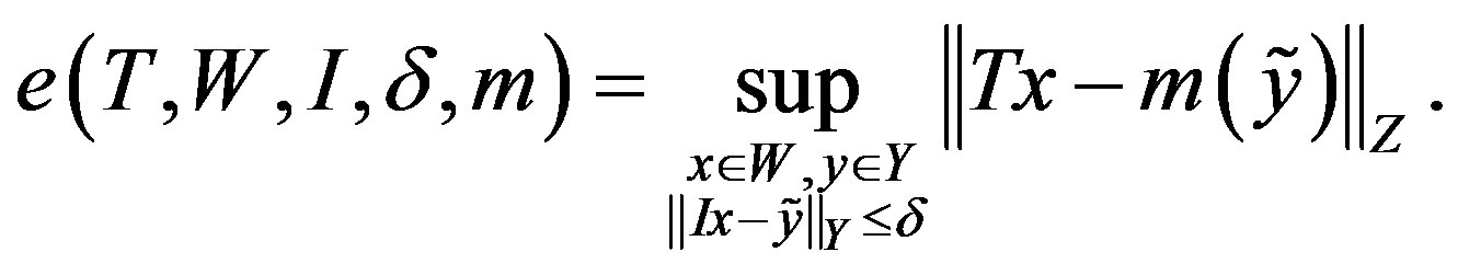
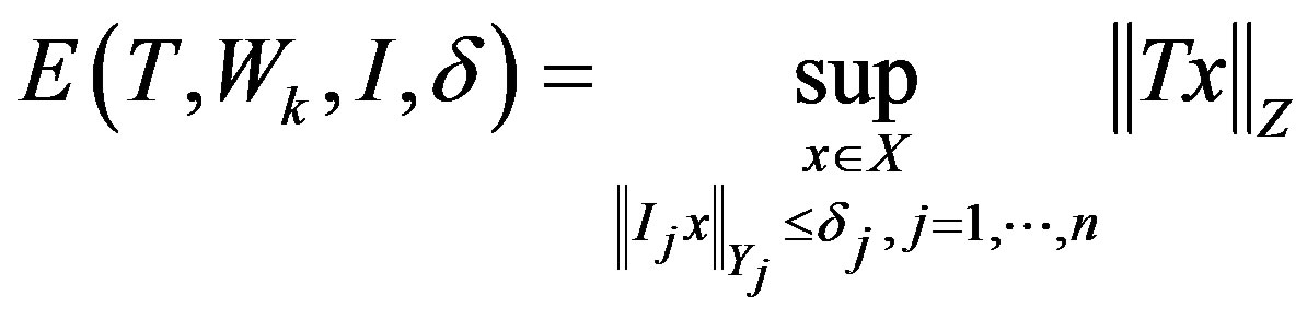
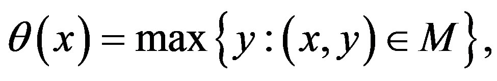
  chosen. So the error of any single method is defined as the worst case error
Now the optimal error is that of the method with the smallest error. Thus the error of optimal recovery is defined as
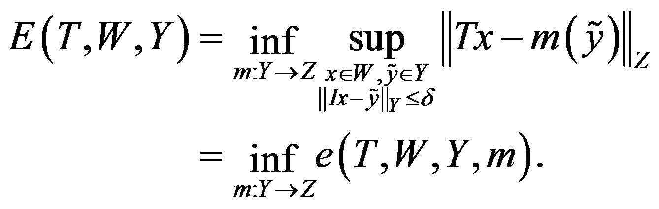 (2)
(2)
For the problems addressed in this paper, let  be linear spaces with semi-inner norms
  and
and  linear operators,
 . We want to recover
  for
for
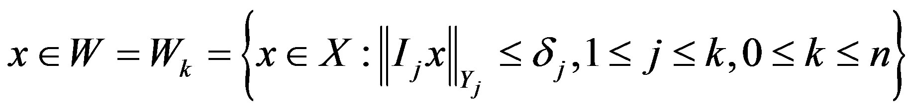
(where if  we let
 ), if we know the values
 satisfying
  for
for .
.
Define the extremal problem
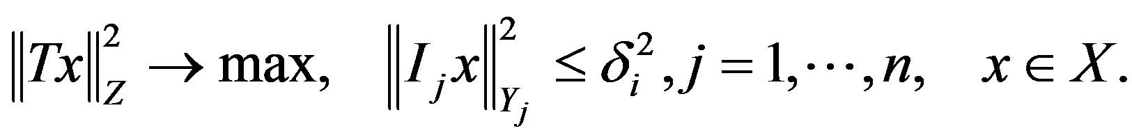 (3)
(3)
This problem is dual to (2).
2. Construction of Optimal Method and Error
The following results of G. G. Magaril-Il’yaev and K. Yu. Osipenko [1] are applied to several problems of optimal recovery.
Theorem 1: Assume that there exist ,
,  such that the solution of the extremal problem
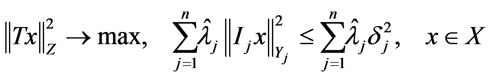 (4)
(4)
is the same as in (3). Assume also that for each
 there exists
 which is a solution to
 (5)
(5)
Then for all ,
,
and the method
 (6)
(6)
is optimal.
Theorem 1 gives a constructive approach to finding an optimal method  from the information. It follows from results obtained in [1-7] (see also [8] where this theorem was proven for one particular case.)
In order to apply Theorem 1 the values of extremal problems (4) and the dual problem (3) must agree. The following result, also due to G. G. Magaril-Il’yaev and K. Yu Osipenko [1], provides conditions under which the solution of problems (3) and (4) will agree.
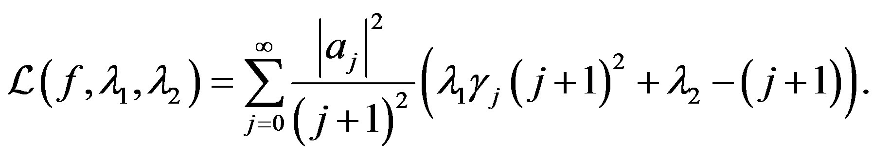
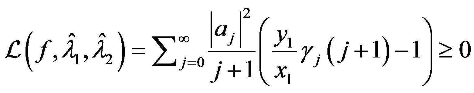
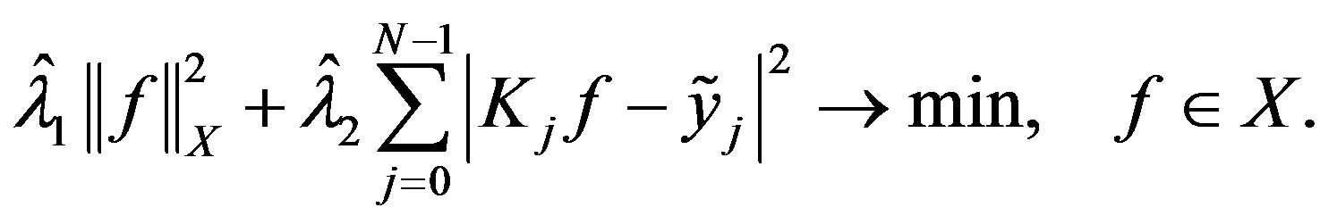
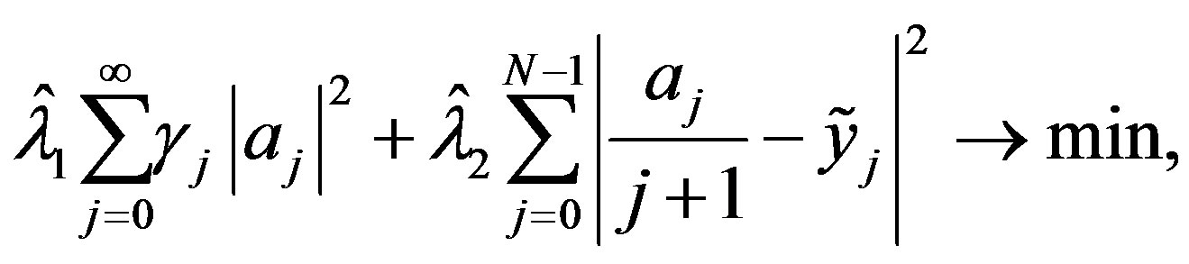
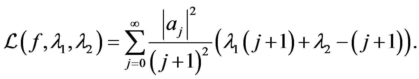
Typically, when one encounters extremal problems, one approach is to construct the Lagrange function . For an extremal problem of the form of (4), the corresponding Lagrange function is

Furthermore,  is called an extremal element if
 for
for  and thus admissible in (4)
and
Theorem 2: Let  and
and  be such that
 for
for  and 1)
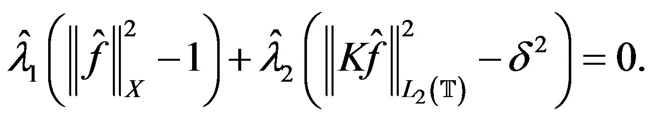
2) 
Then  is an extremal element and
If we wish to combine Theorems 1 and 2 to determine an optimal error and method then we must show the posed problem is able to satisfy equating extremal problems (3) and (4). Through Theorem 2 we have such a means available.
3. Main Results
Consider the class of functions defined on the unit disc  given by
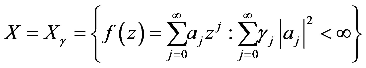 (7)
(7)
for ,
,  satisfying
 (8)
(8)
and
 (9)
(9)
Therefore, any  is holomorphic in the unit disc by (6). We define the semi-norm in
  as
as
and
 (10)
(10)
Let ,
,  , be a linear operator given by
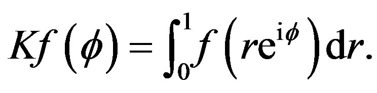
That is,  is the radial integral of
 . To see that
 , by (7) we have for all but finitely many
 ,
,
 for some
 . Thus if
  then
then
 .
.
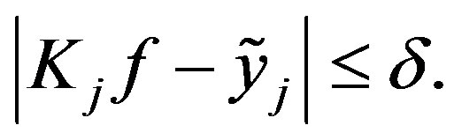
We assume to know  given with a level of accuracy. That is, for a given
 , we know a
  such that
 (11)
(11)
The problem of optimal recovery is to find an optimal recovery method of the function  in the class
  from the information
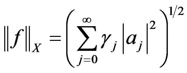
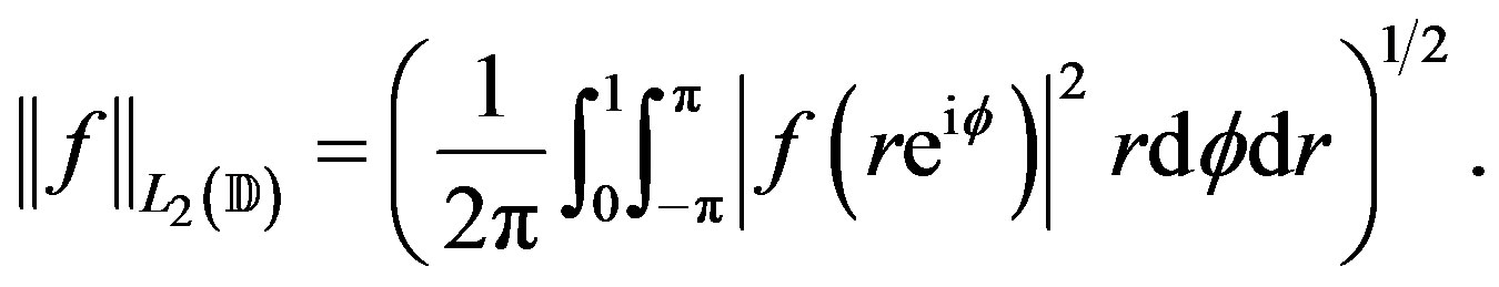
  satisfying (9). The error of a given method is measured in the
  norm defined by
Any method  is admitted as a recovery method. Let
  be sequences of non-negative real numbers such that
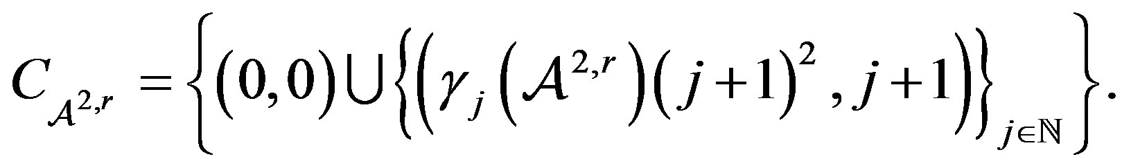
Define  to be the convex hull. Define
  for
for  by
by
Lemma 1: The piecewise linear function  with points of break
 , with
  for
for  given by
  is such that
 .
.
Proof. Assume that  It means that
 . Since
  and
and  as
as  there is a
  such that
  and
and . Then the interval between
  and
and  belongs to
 . Consequently,
  and
and  is not a point of break of
 .
.
Assume that . Since
  the interval between
  and
and  belongs to
 . Geometrically, the line
  to
to  will lie above the line
 . It means that
  contradicting that
  is a point of break of
 .
.
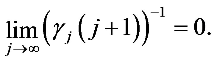
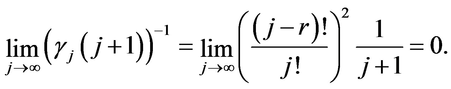
Note that as  then for any fixed
  the slopes between points
  and
and  also tends to 0 as
3.1. Inaccuracy in  Norm
Norm
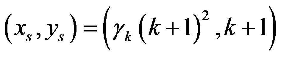
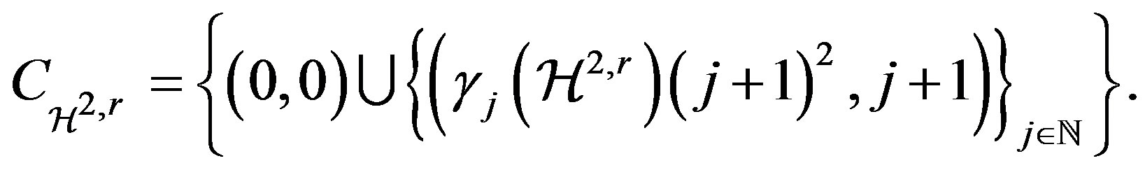
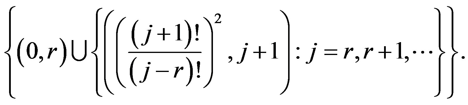
Consider the points in  given by
 and define the convex hull of the origin and this collection of points as
 :
:
 (12)
(12)
Let
 (13)
(13)
thus  is a piecewise linear function. Let
 ,
,  be the points of break of
  with
with . By (7) the assumption for Lemma 1 is satisfied by
  and
and .
.
Theorem 3: Suppose that  with
with  . Let
. Let
 (14)
(14)
Then the error of optimal recovery is
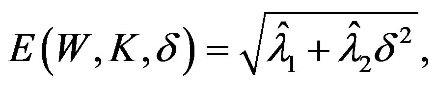 (15)
(15)
and
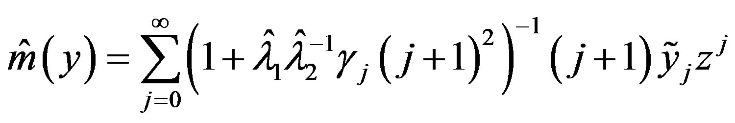 (16)
(16)
is an optimal method of recovery. If  then
then
 and
and  is an optimal method.
Proof. Consider the dual extremal problem
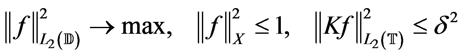 (17)
(17)
which can be written as
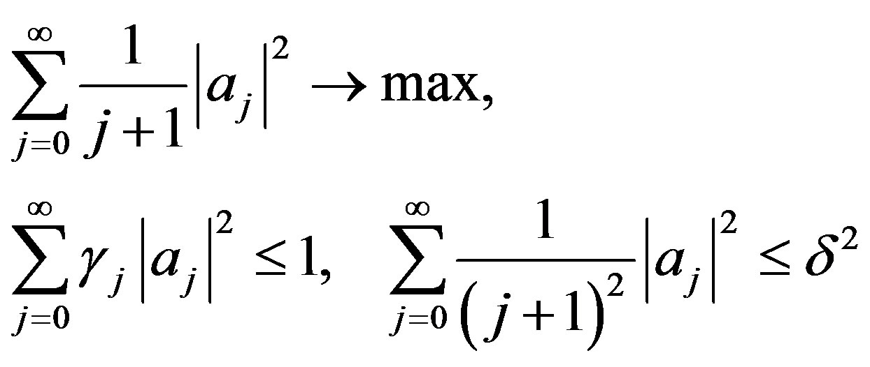
where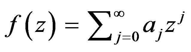 . Define the corresponding Lagrange function as
Let the line segment between successive points
 and
and  be given by
 .
.
That is . Thus
  are given by (12). Take any
 , then by definition of the function
  we have
Thus for all 
and hence  for any
 .
.
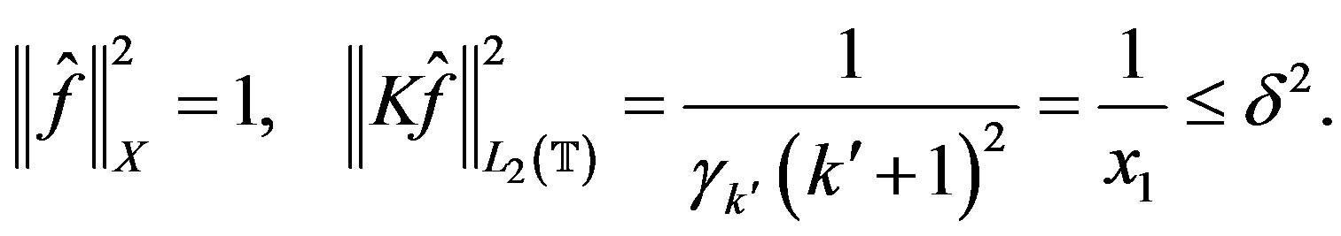
We proceed to the construction of a function  admissable in (15) that also satisfies
 Assume
 .
.
As  if and only if
  and
and  then
then  if and only if
  or
or . Let
. Let  be the indices that satisfy
and
 .
.
We let  for
for , and choose
  so that they satisfy the conditions
 (18)
(18)
From these conditions let
 (19)
(19)
and
 (20)
(20)
Now if  with
with  or
or  and
and
 the function
  is admissible in (15) and
 , that is
  minimizes
and condition 1) of Theorem 2 is satisfied. Furthermore, by construction,  satisfies condition 2) of Theorem 2.
If , that is
  and
and , define
  as in (17). Then as
So let  and we have
Thus the function  is admissable in (15) and satisfies 1) and 2) of Theorem 2. It should be noted that in this case
  are simply
  and
and .
.
Now we proceed to the extremal problem
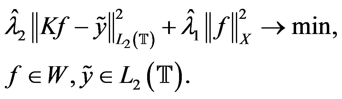 (21)
(21)
This problem may be rewritten as
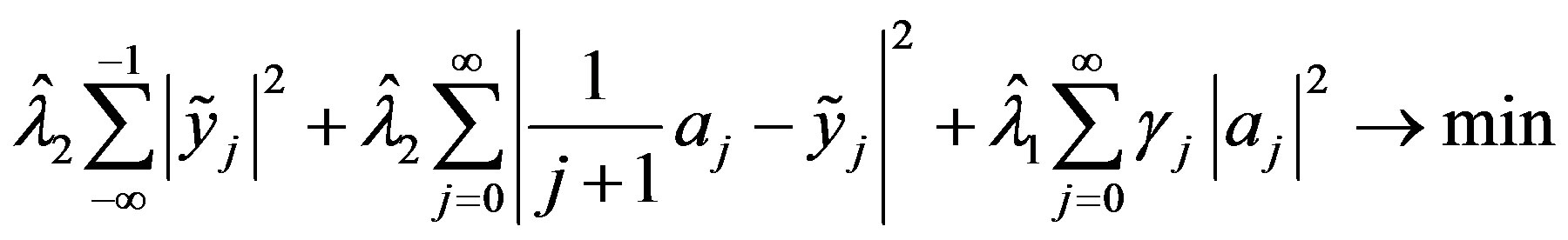
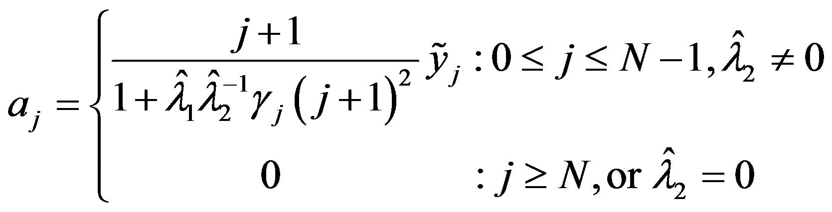
which has solution
So for ,
,  by Theorems 1 and 2, (14) is an optimal method and the error of optimal recovery is given by (13). If
  then
then
 and
and  is an optimal method.
It should be noted that for fixed , that is for a fixed
 , the terms
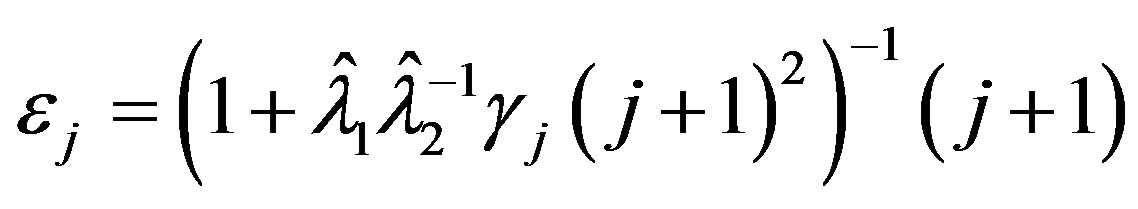
will have the property,  and
and  as
as . So
. So  smooths approximate values of the coefficients of
  by the filter
 .
.
3.2. Inaccuracy in  Norm
Norm
Our next problem of optimal recovery remains to recover  from inaccurate information pertaining to the radial integral of f. However, the inaccurate information we are given are the values
 such that
where  is the
  coefficient of the radial integral
 ,
,
Denote
We again consider the space of functions  given by (5) and
  and
and  defined by (10) and (11) respectively but now add the condition
 (22)
(22)
The problem of optimal recovery on the class  given by (8) is to determine the optimal error
 (23)
(23)
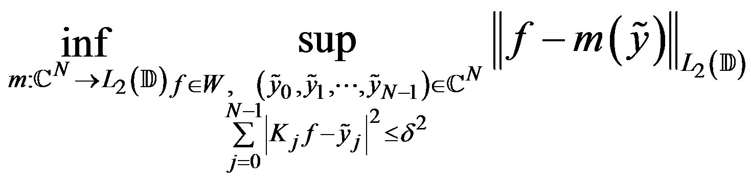 (24)
(24)
and an optimal method  obtaining this error.
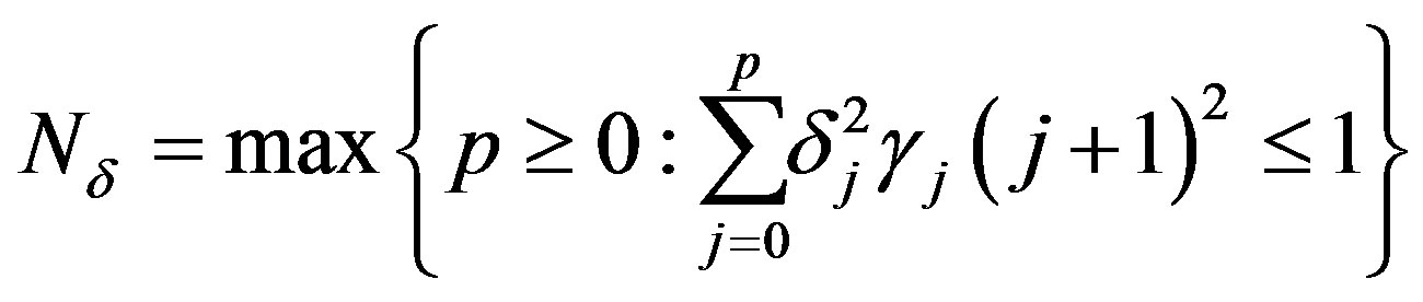
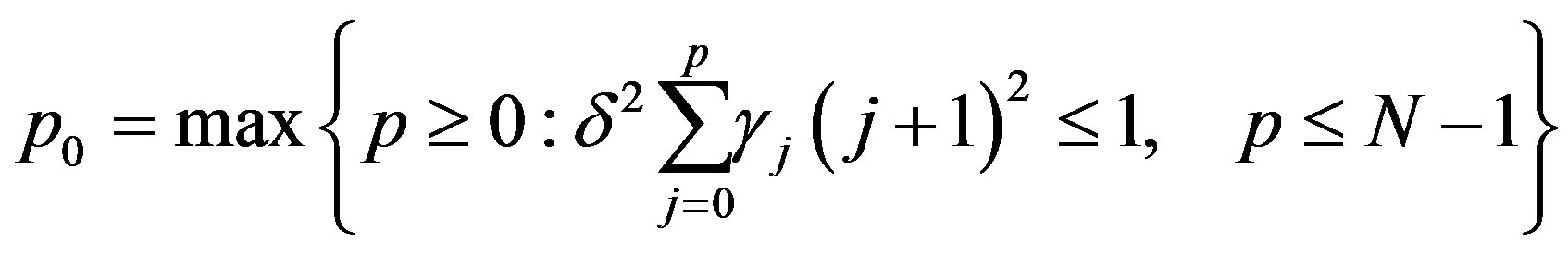
Define  as the largest index such that
 (25)
(25)
which by (7) exists, and
 (26)
(26)
Theorem 4: Suppose  with
with . If
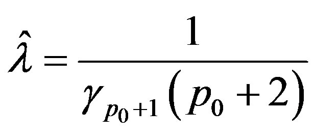
. If
 let
let  and
and .
.
Then the optimal error is
 (27)
(27)
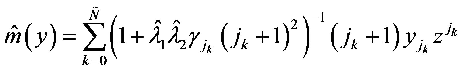
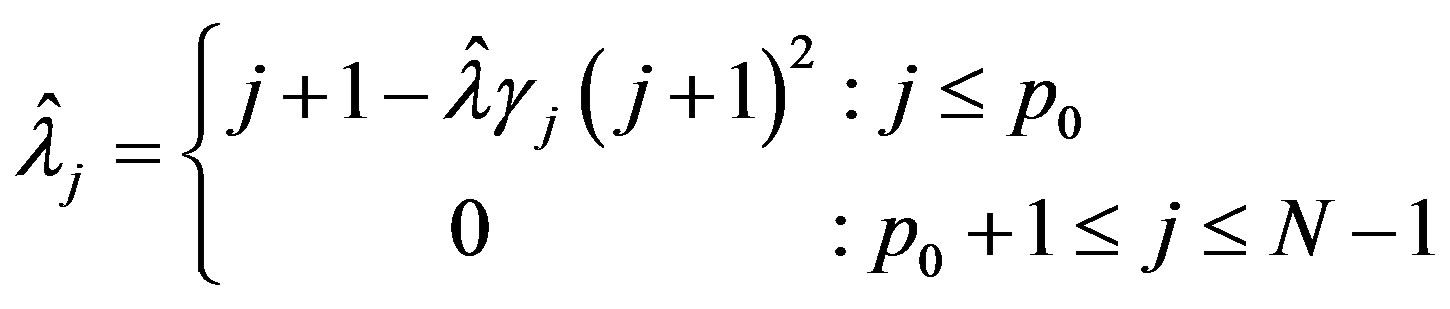
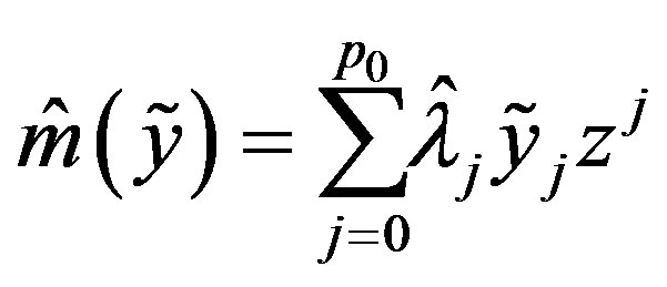
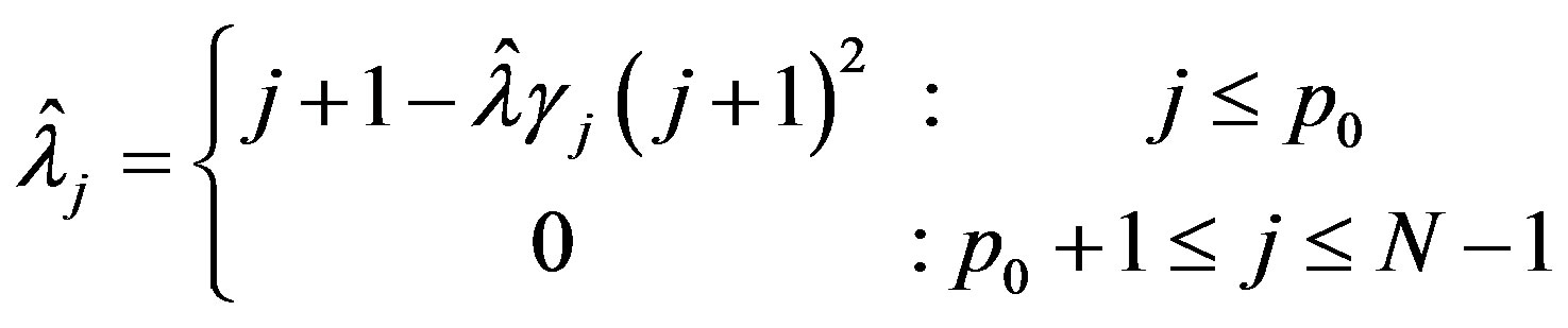
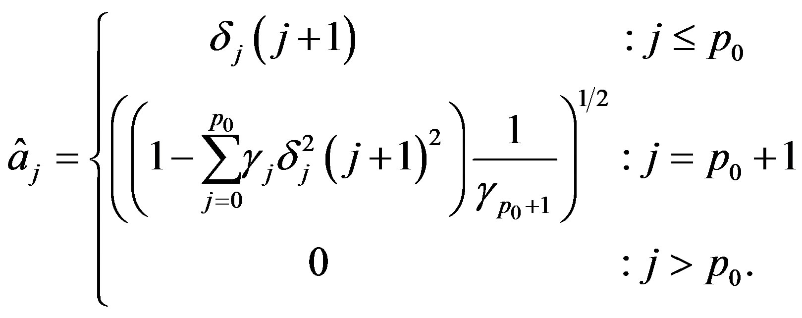
and
 (28)
(28)
is an optimal method. If  then
then
 and
and  is an optimal method.
If  and
and  then with
 and
and  the error of optimal recovery is (22) and (23) is an optimal method. For
 ,
,  and
and  is an optimal method.
Proof. For the cases  with
with  we simply apply the same structure of proof as in Theorem 3. For the case
  there remains some work.
Our construction will depend on whether or not , that is whether or not
  with
with
 .
.
First we notice . Assume not. Then if
  we also know
  since for all
  we assumed
 . Since
  we know
 . Then by definition of
  we know for
 ,
,
and substituting  we have
which contradicts the definition of . Therefore
 and if
  then
then
 .
.
In either case,  or
or , the dual problem is of the form
 (29)
(29)
The corresponding Lagrange function is then
where  is the characteristic function of
 .
.
Case 1): 
If  let
let  correspond to the index satisfying
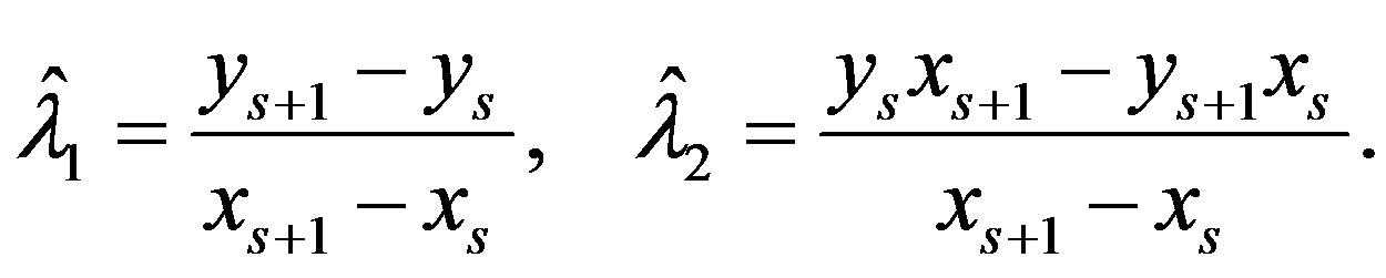
To determine  let
let  be the line through the point
  that is parallel to the line from the origin to
 . That is, let
 (30)
(30)
So for any point of break we have  and for any index
 , we obtain
If  then
then
Thus for the chosen  and
and  and any
  we have
 .
.
To construct  admissable in (24), let
  for
for  and define
  by the system
and since  this becomes
So let  and
and .
.
Then for  the function
 is admissable in (24) with
Therefore  and by construction we have
  and
and 
so that
and conditions (a) and (b) of Theorem 2 are satisfied.
Case 2): 
If  then
then , and
, and , as this is the only point in the set
 with a
  -coordinate of
 . Furthermore, as
  is a point of break of
  we know
  for all
 . Since
  then by the definition of
  we know
 . As
. As
 (31)
(31)
then we obtain equality, .
.
Define  by (25) so
  and
and . If we let
  be
be 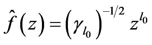 then
then
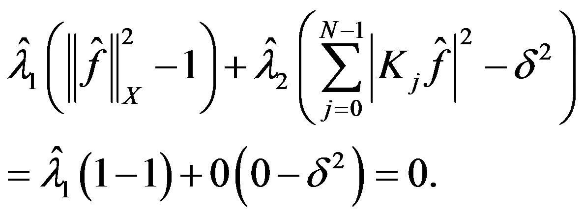
In addition  is admissable in extremal problem (24)
as 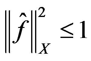 and
and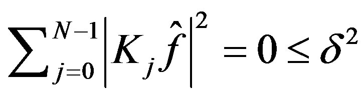 .
.
To justify  simply note that as
 satisfies (26) and
  for all
  then
then
 . So we have
 . Since
 then
then  minimizes
 .
.
For both cases, we now consider extremal problem
 (32)
(32)
This problem can be written as
which will have solution
So by Theorems 1 and 2 we have obtained the optimal error and an optimal method for all scenarios. In each case i and ii,  and
and  are given by (25). In each case, the error of optimal recovery is
 which for case 2) simplifies to
 . Also for each case, a method of optimal recovery is given by
  where in case 2) this simplifies to
  since in case 2),
 .
.
One may be able to reduce the amount information needed without affecting the error of optimal recovery. Therefore, by reducing the number of terms in the optimal method we reduce the compututaions needed. The following ideas are in [9]. We consider the subset ,
,  as the set of all points whose slope to the origin is greater than the slope of
  for
for , that is the slope of the line segment between points
  and
and . Define the sets
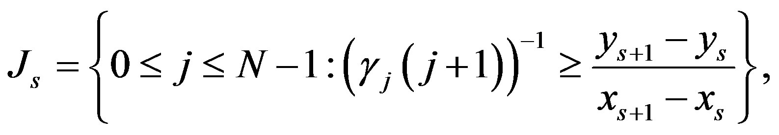 (33)
(33)
for  where if
  define
 . Now consider the same problem as stated in Theorem 4 using only information
 . For
. For
 , we have
  and so
 . In this situation,
  with
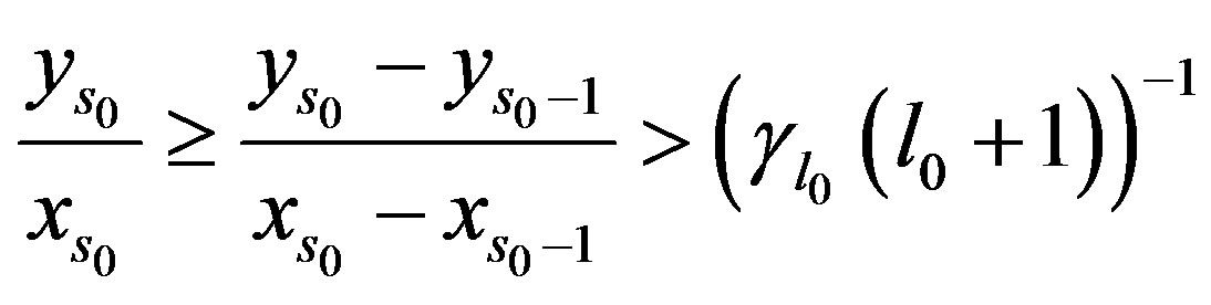
with , it was shown that the error of optimal recovery only involves the two points
 then the reduction in information from
  to
to  will not change the error. That is
 and if
 , an optimal method is
 (34)
(34)
where .
.
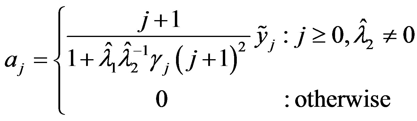
3.3. Varying Levels of Accuracy Termwise
In Theorems 3 and 4 the inaccuracy of the information given is a total inaccuracy. That is, the inaccuracy  is an upper bound on the sum total of the inaccuracies in each term, be it a finite or infinite sum. For Theorems 3 and 4 however, there is no way to tell how the inaccuracy is distributed. In particular, with regards to Theorem 4, the situations in which the given information
  satisfies

or for some particular  satisfying
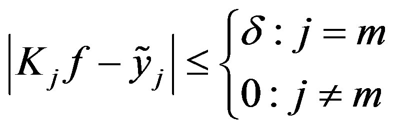
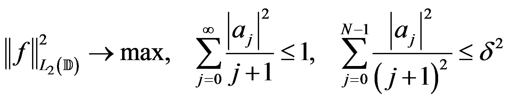
are treated the same. For the next problem of optimal recovery we address this ambiguity. The problem of optimal recovery is to determine an optimal method and the optimal error of recovering , from the information
  satisfying
for some prescribed  and
and .
.
To define  use conditions (6) and (20) as previously but impose an additional restriction. We add the condition
Define  where
where  are the levels of accuracy. If
  define
 (35)
(35)
So  and furthermore
 . The case
  will be treated seperately.
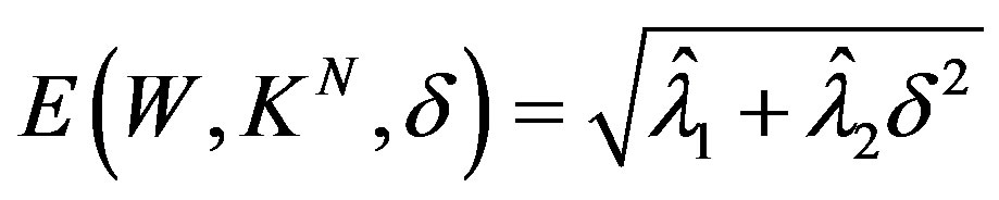
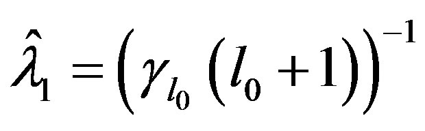
Theorem 5: If  let
let
 (36)
(36)
then the error of optimal recovery is given by
 (37)
(37)
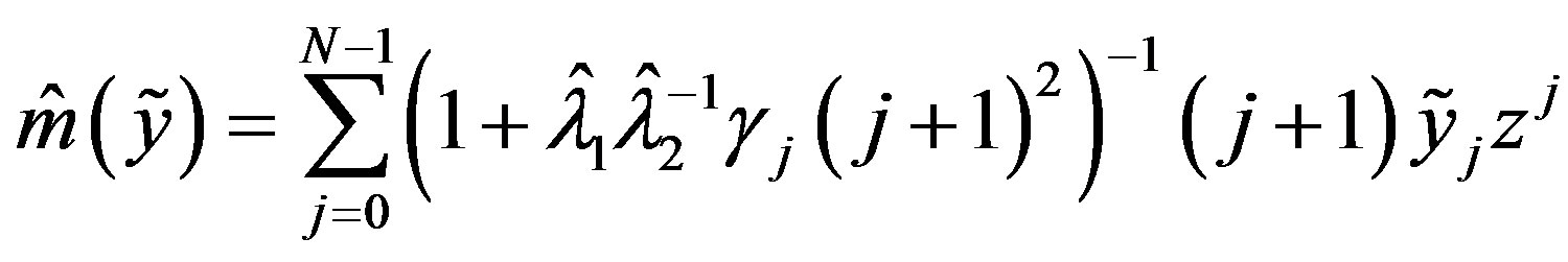
and
 (38)
(38)
is an optimal method.
If  then
then  and
and  is an optimal method.
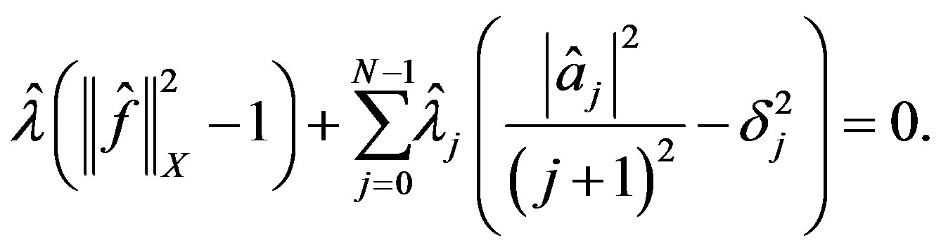
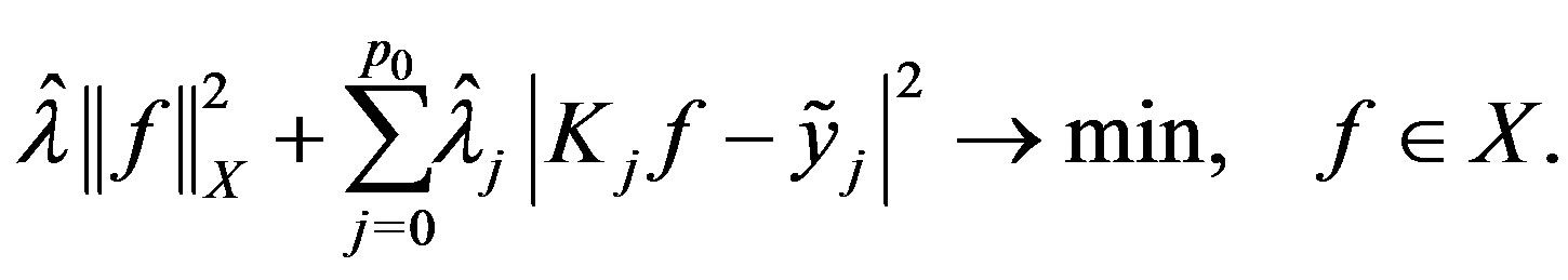
Proof. The dual problem in this situation is
 (39)
(39)
 (40)
(40)
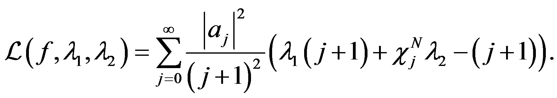
with the corresponding Lagrange function
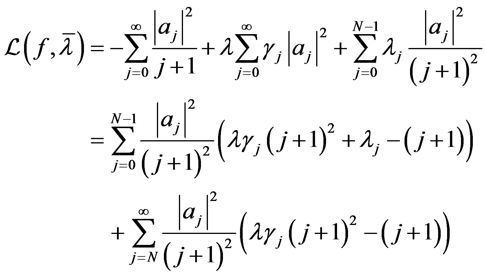
The method of proof will be to first determine
 with
with  and
and  admissable in (31) and satisfying 1) and 2) of Theorem 2.
If , define
  and
and  as follows:

To verify  assume
  in which case
 and hence
To show for the chosen  and any
 ,
,
 , we consider the cases
  or
or .
.
For  we know by assumption
 and hence
For 
Thus for any ,
, . For the constructed
 , it can be shown that
  as desired. and thus
  minimizes the Lagrange function.
To show  is admissable in (31) we can clearly see that for
 ,
, . It remains to show
  for
for . Assume not, then
which occurs if and only if
which contradicts the definition of  unless
  . If
. If  then
then  and hence we no longer need the condition
  in order for
  to satisfy (31).
Furthermore
and so  is admissable in (31).
By the construction of  we also have the results
 and
and  for
for  while
while 
for . Thus
  satisfies 2) of Theorem 2 as
We now proceed to the extremal problem
Notice the upper bound on the sum is  as
as  for any
 . This extremal problem will have solution
Therefore the error of optimal recovery is given by
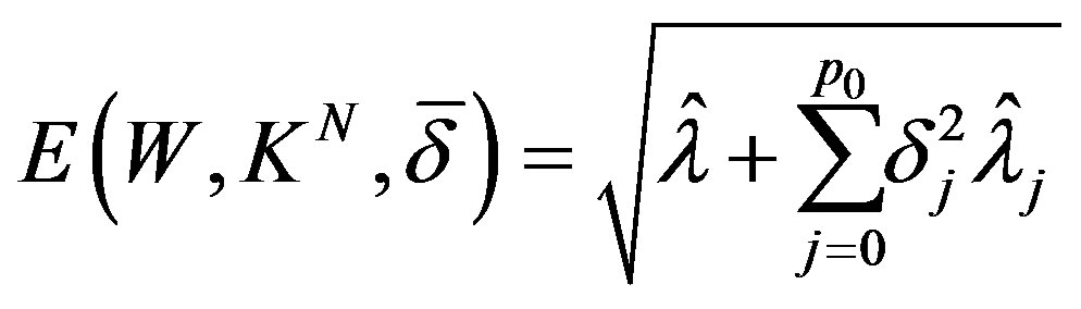
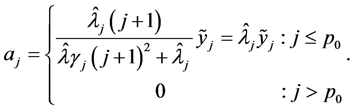
and

is an optimal method.
Now we proceed to the case . Choose
  and
and  for
for . Then as
  for all
Thus  for all
 . Let
. Let 
and  and notice
  and clearly
 so
so  is admissable in (31). Furthermore
and so . Also,
Therefore  and
and 
is an optimal method. 
The optimal method may not use all of the information provided as  may be less than
 . Thus increasing
  may not change
  and hence not change the error or the method. If
 , then
and we can reduce the amount of information needed for a given optimal error.
If  we may be able to reduce the error of optimal recovery if we have more information available. Fix
 . The greater number of terms we have of
  then the better we may be able to approximate
 , that is the smaller the optimal error of recovery. Let
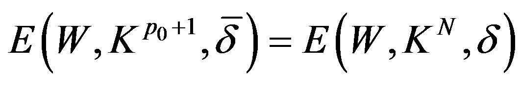
 (41)
(41)
and for 
for any . If we know the first
  terms with some errors, then further increasing the terms will not yield a decrease in the error of optimal recovery.
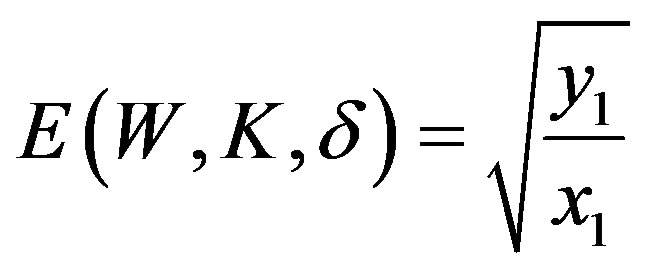
3.4. Applications: The Hardy-Sobolev and Bergman-Sobolev Classes
We now apply the general results to the Hardy-Sobolev and Bergman-Sobolev spaces of functions on the unit disc. Let  denote the set of functions holomorphic on the unit disc. Define the Hardy space of functions
 as the set of all
 ,
,  with
with  where
where
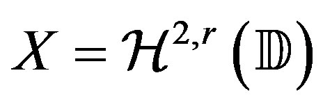
The Hardy-Sobolev space of functions,  , are those
  such that
  and
and
 is the class consisting of those
with . The Bergman space of functions
 is the space of all
  such that
That is,  is the space of all holomorphic functions in
 . The Bergman-Sobolev space of functions,
  , consists of
  with
with
 and
and  as the class of all
 with
with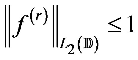 .
.
So each space can be considered as the space  with
with
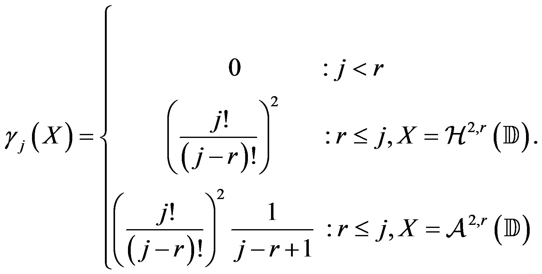
For each space of functions we have the collection of points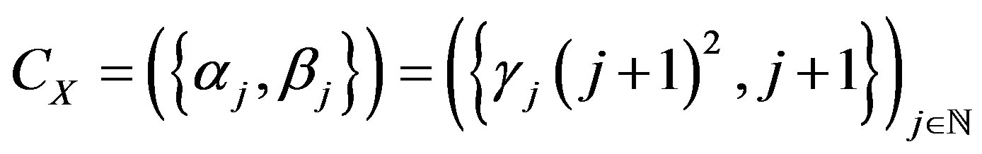 . If
. If
 then for
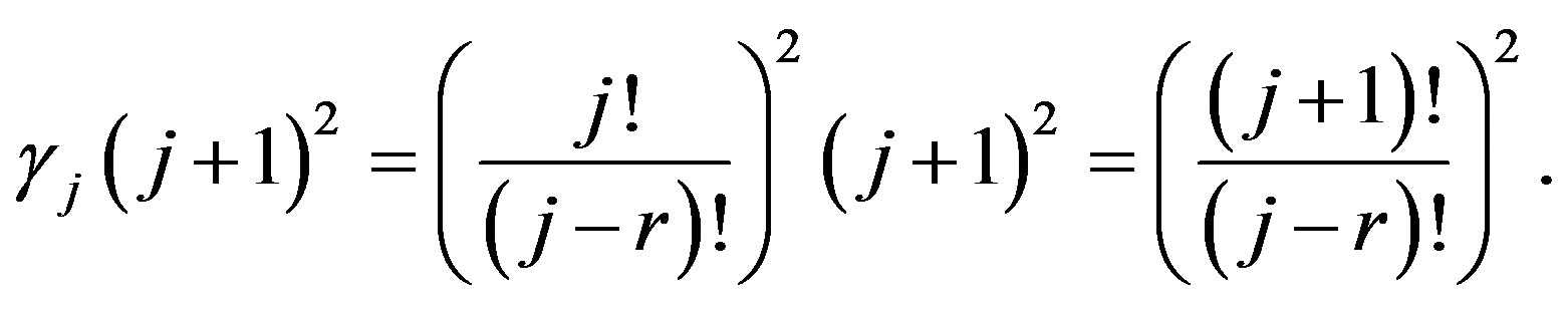
Therefore for 
In this case we consider the collection of points
It is easy to see that if  then the piecewise linear function
  will have points of break
 (42)
(42)
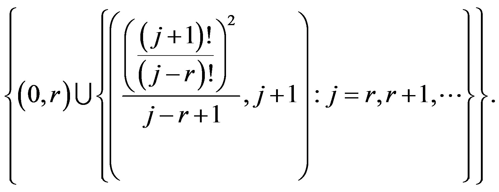
For the space , the points to consider are
Again let 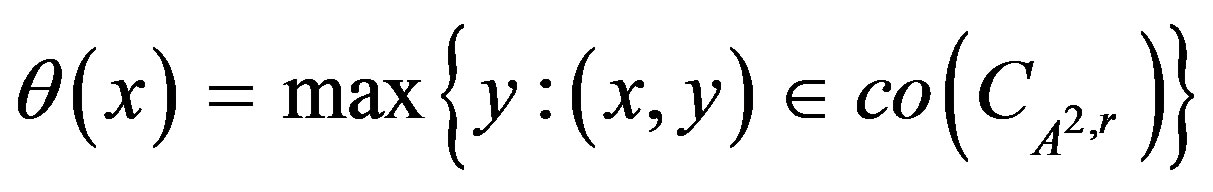 and thus the points of break of
  will be precisely
For the special case of , the function
  has only a single point of break at the origin as
so that  for
for . Furthermore,
  does not satisfy (7) as
Thus, in the applications of the general results, this case will be treated separately.
For notational purposes, let ,
,  be the points of break of
  for the space
 .
.
Corollary 1. Let  or
or . If
. If  with
with  or
or  then the error of optimal recovery is given by (13) and (14) is an optimal method. If
  and
and  then
then  and
and  is optimal.
Proof. For the spaces  or
or ,
,  if and only if
  and
and . Thus
  if and only if
  or
or . Thus apply Theorem 3 to obtain the result for all spaces except
 . The dual problem in the case
  leads to a simple Lagrange function. The dual problem is specifically
Therefore the Lagrange function is simply given by
Now if we let  and
and  then
then
 for any
 . So now proceed as in Theorem 3. As any
  will minimize
 , choose
  as in (18). The extremal problem (19) is solved similarly, and as
  then
then  for
for .
. 
It should be noted that the optimal method described is stable with respect to the inaccurate information data.
We now apply Theorem 4 to the Hardy-Sobolev spaces  and Bergman-Sobolev spaces
  in which
  is explicitly defined to be the smallest nonnegative integer satisfying
For the case ,
,  for all
 . Thus
  does not depend on
 . So
. So
 and hence for any
  we are in the case
 .
.
Corollary 2. Let  or
or . Suppose
  with
with . If
. If  or
or  then let
 be given by (12) and the optimal error is given by
(13) and (23) is an optimal method. If  and
and  then
then  and
and  is an optimal method.
Otherwise suppose . If
. If  or
or  then the optimal error is given by (13) and (23) is an optimal method with
  and
and
 . If
. If  and
and  then
then
 and
and  is an optimal method.
Proof. As previously stated, if  the only break point of
  is
is  and furthermore as
 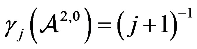 then
then  given by (21) does not exist so we treat this special case. In this case, the dual extremal problem is
and the corresponding Lagrange function is simply
If  and
and  then
then  for any
 . Now proceed as in the proof of Theorem 4 to obtain the result.
We now apply Theorem 5 to the spaces  or
or  for
for . In this situation
  will be a non-decreasing sequence for all
 . Also, for any
  we have
  and we are always in the case
 . For
. For  then for both the Hardy and Bergman spaces
  and so the condition
  will be satisfied if we know
  satisfying
Corollary 3. Let  or
or  with
with  or
or  and
and  and
and  given by (27). Let
 ,
,  be given by (28). Then the error of optimal recovery is given by (29) and (38) is an optimal method. If
  and
and  then
then  and
and  is an optimal method.
Proof. For Theorem 5 we simply used conditions (6) and (20), both of which are satisfied by  and
and  for all
 .
.
As a direct consequence of Theorem 5, we consider the situation in which we have a uniform bound on the inaccuracy of each of the first  terms of
 . That is we take
  for every
 . If
. If  we define
  similarly as
and the apriori information is given by the values  such that
Again we will only need the values  for an optimal method.
As previously noted, since the optimal method and error of optimal recovery only use up to the  term then any information beyond may be disregarded if
  as additional information will not decrease the error of optimal recovery.
REFERENCES
- K. Y. Osipenko, “Optimal Recovery of Linear Operators from Inaccurate Information,” MATI-RSTU, Department of Mathematics, Washington DC, 2007, pp. 1-87.
- G. G. Magaril-Il’yaev and K. Y. Osipenko, “Optimal Recovery of Functions and Their Derivatives from Fourier Coefficients Prescribed with an Error,” Sbornik: Mathematics, Vol. 193, No. 3, 2002, pp. 387-407.
- G. G. Magaril-Il’yaev and K. Y. Osipenko, “Optimal Recovery of Functions and Their Derivatives form Inaccurate Information about the Spectrum and Inequalities from Derivatives,” Functional Analysis and Its Applications, Vol. 37, No. 3, 2003, pp. 203-214. doi:10.1023/A:1026084617039
- A. G. Marchuk and K. Y. Osipenko, “Best Approximations of Functions Specified with an Error at a Finite Number of Points,” Mathematical Notes of the Academy of Sciences of the USSR, Vol. 17, No. 3, 1975, pp. 207- 212. doi:10.1007/BF01149008
- A. A. Melkman and C. A. Micchelli, “Optimal Estimation of Linear Operators in Hilbert Spaces from Inaccurate Data,” SIAM Journal on Numerical Analysis, Vol. 16, No. 1, 1979, pp. 87-105. doi:10.1137/0716007
- K. Y. Osipenko, “Best Approximation of Analytic Functions from Information about Their Values at a Finite Number of Points,” Mathematical Notes of the Academy of Sciences of the USSR, Vol. 19, No. 1, 1976, pp. 17-23. doi:10.1007/BF01147612
- K. Y. Osipenko, “The Hardy-Littlewood-Polya Inequality for Analytic Functions from Hardy-Sobolev Spaces,” Sbornic: Mathematics, Vol. 197, No. 3, 2006, pp. 315- 334.
- K. Y. Osipenko and M. I. Stessin, “Hadamard and Schwarz Type Theorems and Optimal Recovery in Spaces of Analytic Functions,” Constructive Approximation, Vol. 31, No. 1, 2009, pp. 37-67.
- K. Y. Osipenko and N. D. Vysk, “Optimal Recovery of the Wave Equation Solution by Inaccurate Input Data,” Matematicheskie Zametki, Vol. 81, No. 6, 2007, pp. 723- 733.