American Journal of Computational Mathematics
Vol.2 No.3(2012), Article ID:23165,21 pages DOI:10.4236/ajcm.2012.23023
A Spectral Method in Time for Initial-Value Problems
Division of Fusion Plasma Physics, Association EURATOM-VR, Alfvén Laboratory, School of Electrical Engineering, KTH Royal Institute of Technology, Stockholm, Sweden
Email: jan.scheffel@ee.kth.se
Received April 27, 2012; revised June 22, 2012; accepted June 29, 2012
Keywords: Initial-Value Problem; WRM; Time-Spectral; Spectral Method; Chebyshev Polynomial; Fluid Mechanics; MHD
ABSTRACT
A time-spectral method for solution of initial value partial differential equations is outlined. Multivariate Chebyshev series are used to represent all temporal, spatial and physical parameter domains in this generalized weighted residual method (GWRM). The approximate solutions obtained are thus analytical, finite order multivariate polynomials. The method avoids time step limitations. To determine the spectral coefficients, a system of algebraic equations is solved iteratively. A root solver, with excellent global convergence properties, has been developed. Accuracy and efficiency are controlled by the number of included Chebyshev modes and by use of temporal and spatial subdomains. As examples of advanced application, stability problems within ideal and resistive magnetohydrodynamics (MHD) are solved. To introduce the method, solutions to a stiff ordinary differential equation are demonstrated and discussed. Subsequently, the GWRM is applied to the Burger and forced wave equations. Comparisons with the explicit Lax-Wendroff and implicit Crank-Nicolson finite difference methods show that the method is accurate and efficient. Thus the method shows potential for advanced initial value problems in fluid mechanics and MHD.
1. Introduction
Initial-value problems are traditionally solved numerically, using finite steps for the temporal domain. The time steps of explicit time advance methods are chosen sufficiently small to be compatible with constraints such as the Courant-Friedrich-Lewy (CFL) condition [1]. Implicit schemes may use larger time steps at the price of performing matrix operations at each of these. Semiimplicit methods [2,3] allow large time steps and more efficient matrix inversions than those of implicit methods, but may feature limited accuracy. These methods nevertheless provide sufficiently efficient and accurate solutions for most applications. For applications in physics where there exist several separated time scales, however, the numerical work relating to advancement in the time domain can become very demanding. Another computational issue is that it may be advantageous to determine parametrical dependences without performing a sequence of runs for different choices of parameter values.
We here outline a fully spectral method for computing semi-analytical solutions of initial-value partial differenttial equations [4]. To this end all time, space and physical parameter domains are treated spectrally, using series expansion. By semi-analytical is meant that approximate solutions are obtained as finite, analytical spectral Chebyshev expansions with numerical coefficients. Important applications are scaling studies, in which the detailed parametrical dependence preferably should be estimated in analytical form. Here the envelope of the characteristic dynamics may often be of higher interest than, for example, fine scale turbulent phenomena. Thus the possibility to filter out, or average, fine structures to obtain higher computational efficiency is a main theme of this work. However, the GWRM may also provide high accuracy when modelling more detailed phenomena. In all cases, the resulting functional solutions are immediately available for differentiation, integration or other analytic subsequent usage.
The GWRM approach consistently employs Chebyshev polynomials for all temporal, spatial and parameter domains for linear and non-linear initial-value problems with arbitrary initial and periodic or non-periodic boundary conditions. As such it appears not to have been extensively pursued earlier. The idea to employ orthogonal sets of basis functions to globally minimize spatial spectral expansions (weighted residual methods, WRM) is, however, far from new [5,6]. The GWRM is indeed a Galerkin WRM, using the weak formulation of the differential equation, as in finite element methods (FEM). An important difference to FEM is the use of more advanced trial functions, valid for larger domains. This is of particular importance for “smearing out” small scale fluctuations.
A number of authors have investigated various aspects of spectral methods in time. Some early ideas were not developed further in [7]. In 1986, Tal-Ezer [8,9] proposed time-spectral methods for linear hyperbolic and parabolic equations using a polynomial approximation of the evolution operator in a Chebyshev least square sense. Later, Ierley et al. [10] solved a a class of nonlinear parabolic partial differential equations with periodic boundary conditions using a Fourier representation in space and a Chebyshev representation in time. Tang et al. [11] also used a spatial Fourier representation for solution of parabolic equations, but introduced Legendre PetrovGalerkin methods for the temporal domain. More recently Dehghan et al. [12] found solutions to the nonlinear Schrödinger equation, using a pseudo-spectral method where the basis functions in time and space were constructed as a set of Lagrange interpolants.
Chebyshev polynomials are used here for the spectral representation in the GWRM. These have several desirable qualities. They converge rapidly to the approximated function, they are real and can easily be converted to ordinary polynomials and vice versa, their minimax property guarantees that they are the most economical polynomial representation, they can be used for nonperiodic boundary conditions (being problematic for Fourier representations) and they are particularly apt for representing boundary layers where their extrema are locally dense [13,14]. The GWRM is fully spectral; all calculations are carried out in spectral space. The powerful minimax property of the Chebyshev polynomials [14] implies that the most accurate n-m order approximation to an nth order approximation of a function is a simple truncation of the terms of order > n-m. Thus nonlinear products are easily and efficiently computed in spectral space. Since the GWRM efficiently uses rapidly convergent Chebyshev polynomial representation for all time, space and parametrical dimensions, pseudospectral implementation [13] has so far not been pursued. The GWRM eliminates time stepping and associated, limiting grid causality conditions such as the CFL condition.
The method is acausal, since the time dependence is calculated by a global minimization procedure acting on the time integrated problem. Recall that in standard WRM methods, initial value problems are transformed into a set of coupled ordinary, linear or non-linear, differential equations for the time-dependent expansion coefficients. These are solved using finite differencing techniques.
The structure of the paper is as follows. First, the GWRM is outlined mathematically. We show, in sections 2-4, how integration, differentiation, nonlinearities, as well as initial and boundary conditions are handled in multivariate Chebyshev spectral space for arbitrary solution intervals. Having transformed the initial-value problem, a set of algebraic equations for the coefficients of the Chebyshev expansions result. These are solved using a new, efficient global nonlinear equation solver which is briefly described in section 5. The introduction of temporal and spatial subdomains, for increasing efficiency, is discussed in section 6. As an introductory example, we solve a stiff, time-dependent ordinary differential equation representing flame propagation. For studying accuracy, the nonlinear Burger equation and its exact solution is used. Detailed comparisons with the time differencing Lax-Wendroff (explicit) and Crank-Nicolson methods (semi-implicit) are presented in section 7. A forced wave equation is subsequently used for studying strongly separated time scales. Finally, we demonstrate application of the GWRM to stability problems formulated within the linearised ideal and resistive magnetohydrodynamic (MHD) models. The paper ends with a summary and conclusions.
2. Generalized Weighted Residual Method
2.1. Method
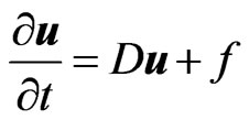
Consider a system of parabolic or hyperbolic initial-value partial differential equations, symbolically written as
 (1)
(1)
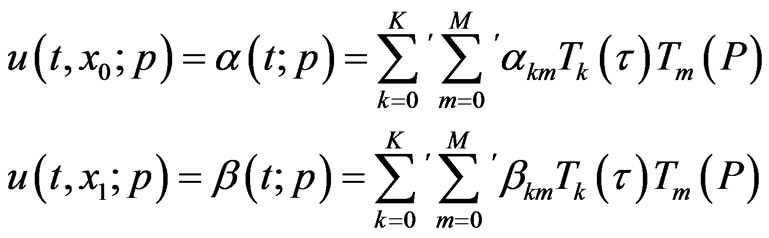
where  is the solution vector, D is a linear or nonlinear matrix operator and
  is an explicitly given source (or forcing) term. Note that D may depend on both physical variables (t, x and u) and physical parameters (denoted p) and that f is assumed arbitrary but non-dependent on u. Initial u(t0, x; p) as well as (Dirichlet, Neumann or Robin) boundary u(t, xB; p) conditions are assumed known.
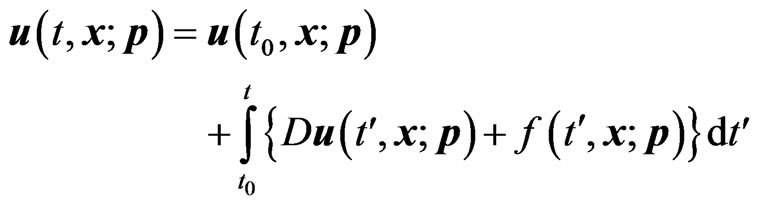
Our aim is to determine a spectral solution of Equation (1), using Chebyshev polynomials [14] in all dimensions. To avoid inverting a matrix solution vector, associated with the time derivative, Equation (1) is now integrated in time. The resulting formulation of the problem is conveniently coupled to the fixed point algebraic equation solver SIR described in Section 5. Thus
 (2)
(2)
The solution  is approximated by finite, multivariate first kind Chebyshev polynomial series. Recall that Chebyshev polynomials of the first kind (henceforth simply referred to as Chebyshev polynomials) are defined by
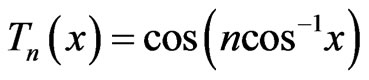 . These functions can be written as real, simple polynomials of degree n and are orthogonal in the interval
  over a weight
 . Thus
 ,
,  ,
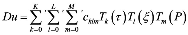
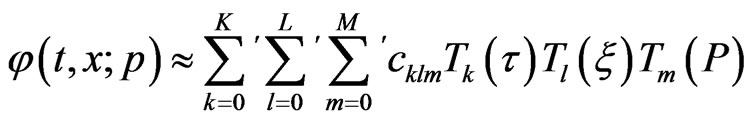
,  etc. For simplicity, we will now restrict the discussion to a single equation with one spatial dimension x and one physical parameter p. Schemes for several coupled equations and higher dimensions may subsequently be straightforwardly obtained. Thus,
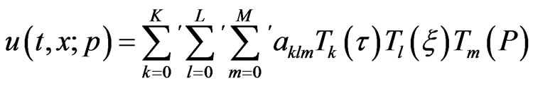 (3)
(3)
with
 (4)
(4)
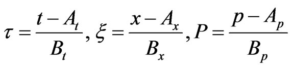
and ,
, . Here z = t, x or p. Indices “0” and “1” denote lower and upper computational domain boundaries, respectively. The basic Chebyshev polynomials have the limited range of variation
  and they require arguments within the same range. The variables
 ,
,  and P used here allow for arbitrary, finite computational domains. We note that, at the spatial boundaries,
  and
and . Primes on summation signs in Equation (3) indicate that each occurence of a zero coefficient index should render a multiplicative factor of 1/2.
Next, we use a weighted residual formulation in order to determine the unknown coefficients aklm of the solution ansatz (3).
2.2. Spectral Coefficients from Weighted Residual Method
The weighted residual method (WRM) is based on the idea that a residual, when using the ansatz (3) in Equation (2), is to be minimized globally. The residual is integrated over the entire solution domain in order to produce a set of equations for the coefficients of Equation (3). In the Galerkin WRM approach, the simplifying continuous orthogonality properties of the basis functions are employed through first multiplying the partial differential equation by basis functions of the same kind as those of the ansatz. Weight functions may also be included. Thus, similarly as for FEM, the weak formulation of the pde is used. The Galerkin WRM of the present method, providing the equations for the coefficients , is
, is
 (5)
(5)
where the residual R is defined as

with
 .
.
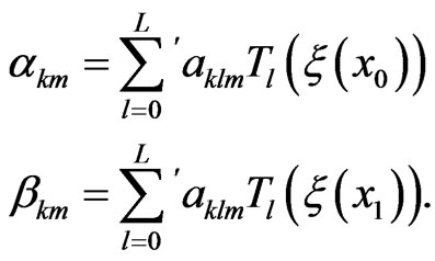
The solution ansatz (3) is now inserted into Equation (5). The separation of variables inherent in the Galerkin WRM approach, enables separately performed integrations. Consequently
 (6)
(6)
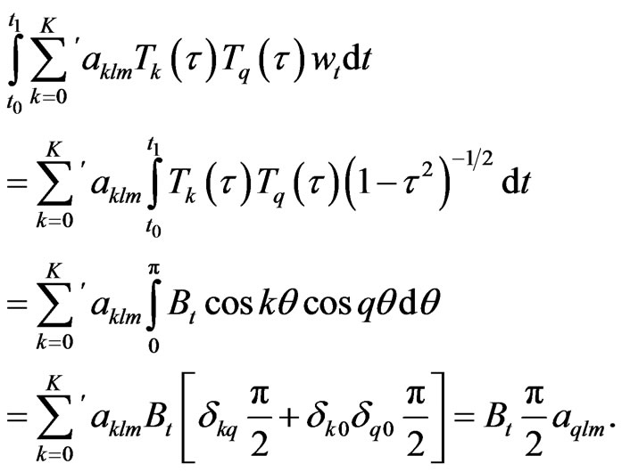
We have used the variable transformation  and introduced the Kronecker delta
  (being 1 if i = k and 0 otherwise). The integrals over the spatial and parameter domains may be computed likewise, and the first term of Equation (5) becomes
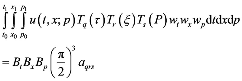 (7)
(7)
where the indices obey 0 ≤ q ≤ K, 0 ≤ r ≤ L, 0 ≤ s ≤ M. For the second term of Equation (5) the initial condition is expanded as
 (8)
(8)
with
 (9)
(9)
where  has been used. We find
 (10)
(10)
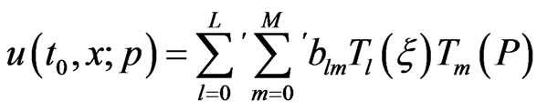
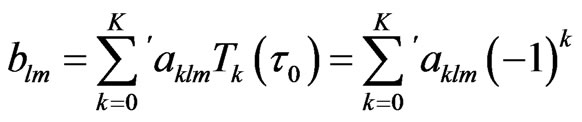
Next, we apply the expansions
 (11)
(11)
which yield
 (12)
(12)
and similarly for the coefficients . The final expression for the GWRM coefficients of Equation (3) becomes simply, using Equations (5), (7), (10) and (12),
 (13)
(13)
defined for all 0 ≤ q ≤ K + 1, 0 ≤ r < LBC, 0 ≤ s ≤ M. Note that the number of modes in the temporal domain is extended to K + 1 due to the time integration, that the initial conditions are included at this stage and that the high end spatial modes with  are saved for implementation of boundary conditions. Since the solution ansatz (3) extends to K temporal modes only, the K + 1 mode needs special attention as discussed below.
It may also be noted that Equation (13), the equation for the Chebyshev coefficients, is the same as that which would obtain if the residual R, using Equations (3), (8) and (11), is set identically to zero. How can the global WRM solution of Equation (13) correspond to a “local” Chebyshev approximation? The explanation is that Chebyshev approximations are not local in contrast to, for example, Taylor series expansions of ordinary polynomials. They are always defined on an interval (see Equations (3) and (4)). Due to the uniqueness given by their minimax property, “local” or “global” Chebyshev approximations are identical once a domain is defined.
Whether solving a single differential equation or a system of coupled linear/nonlinear differential equations, Equation (13) will constitute a set of coupled linear/ nonlinear algebraic equations. Here the coefficients  are themselves functions of the coefficients
  whereas the coefficients
  are uniquely determined from the forcing term f. For example, if f equals a constant C, then
 . This is shown using Equation (11). Thus Equation (13) specifies a complete, implicit relation for the coefficients
  of the solution together with the boundary conditions, which will be discussed in the next section. Methods for efficient iterative solution of Equation (13) will be introduced in section 5. Convergence is controlled by requiring that the absolute values sum of the first few coefficients of the solution (3) deviates less than some value
  from one iteration to the next. Usually we assume
 .
.
2.3. Representation of Integrals and Differentials
By also letting
 (14)
(14)
we may employ the Chebyshev representation of time integration:
 (15)
(15)
If the operator D contains spatial derivatives, the following formulas are used [14]:
 (16)
(16)  (17)
(17)
Note that the coefficients  and
and  are valid for the intervals
  and
and , respectively.
2.4. Truncation and the Minimax Property
The finite number of spectral terms introduces some subtleties. Although Equation (13) may be solved to order K + 1, the solution ansatz (3) is limited to order K. Assuming that K is the highest temporal mode number used in the computation, the term  in the sum of Equation (15) must still be retained so that
  is correctly calculated for a true K order minimax approximation. Since the integrals in Equation (11) are subsequently truncated to order K, the initial condition
  will not be exactly reproduced when setting t = t0 in the solution Equation (3) due to that the integrals will become non-zero (to order K + 1 they are indeed zero). There is, however, a remedy to save both minimax accuracy and true representation of the initial condition. By letting
  everywhere except for on the left hand side of Equation (13), a solution is obtained which exactly reproduces the initial condition for t = t0. We do not give a formal proof here; rather we conjecture (after having studied a few cases) that this solution exactly coincides with the WRM solution produced directly from the original differential form Equation (1). This is not overly surprising, since the information used by both the differential and the integral formulations becomes the same in this case. Both of the procedures discussed are used in this work.
All computations are here performed using the computer mathematics programme Maple, since editing, compilation, linking, execution, plotting and debugging are conveniently performed within the same environment. For some computations, like when solving Equations (13), analytic differentiation and analytic simplification of expressions, being easily carried out in Maple, is desirable. The GWRM is easily coded in numerically efficient languages like Matlab or Fortran. The computational speed per se is not important for the benchmarking and comparisons with other methods given in Section 7; rather it is here more important that all comparisons are carried out within the same computational environment.
3. Boundary and Initial Conditions
We now turn to a discussion of implementation of initial and boundary conditions in the GWRM. Their number depends on the number of equations in (1) and by the order of the spatial derivatives. It is already shown that initial conditions enter directly into Equation (13).
Boundary conditions should be applied at coefficients  at the upper end of the spatial mode spectrum. This can be seen in several ways. From Equations (16), (17) it is clear that the Chebyshev representation of functions differentiated l times is only valid up to order L − l. Thus the coefficient Equations (13) do not apply for higher spatial mode numbers.
Furthermore, it is instructive to consider the flow of information in Chebyshev space, associated with temporal integration and spatial differentiation during iteration of Equation (13); see Figure 1. Note that for differentiation, only higher order modes contribute to the value of the Chebyshev coefficient at a specific modal point
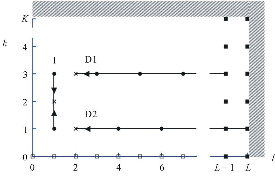
Figure 1. Flow of information in Chebyshev space to a modal point (k, l), associated with the coefficient aklm (the modal point is marked with a cross) from nearby modes when performing integration (I) in time as well as single differentiation (D1) or second differentiation (D2) in space. Modes that are used for implementing initial conditions (empty squares) and boundary conditions (filled squares) are also indicated (two boundary conditions are shown).
whereas for integration, the Chebyshev coefficient at modal point k samples information from modal points both at k − 1 and k + 1. Modes that contribute to the values of the integral or derivatives are marked. Modes outside the computational domain (dashed region and beyond) are defined to give zero contribution. The spatial domain behaviour is consistent with that the solution (13) is defined only to spatial orders less than . Thus L − LBC is the number of boundary conditions that should be imposed for all k and m.
In the diagram, modal points used for two boundary conditions are shown (filled squares). It is seen that any error occuring at high spatial mode numbers is amplified through the multiplicative terms in Equations (16), (17), and numerical instability could result. Since Chebyshev coefficients usually converge rapidly with mode numbers and since the boundary conditions are considered known, numerical stability is usually not compromised by this effect.
The initial condition is imposed at k = 0 for all modes with 0 ≤ l < LBC ≤ L and 0 ≤ m ≤ M and are marked by empty squares. The initial condition may be chosen arbitrarily. If the initial condition requires many, or all, temporal modes for sufficient resolution, care must be taken not to conflict with the boundary conditions applied at high l values. Preferably, initial conditions are chosen so that they satisfy the boundary conditions.
Chebyshev Expansion of Boundary and Initial Conditions
The boundary conditions are implemented into the GWRM in the following way. We chose here to describe the case of Dirichlet boundary conditions; one at each end of a 1D spatial interval. Other types of boundary conditions may straightforwardly be implemented once this case is understood. For systems of equations with many boundary equations, subroutines for handling this are preferably programmed. The boundary conditions are Chebyshev expanded as
 (18)
(18)
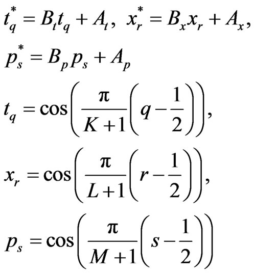
We choose to apply discrete Chebyshev interpolation both for initial and boundary conditions since this procedure has precisely the same effect as taking the partial sum of a Chebyshev series expansion and is easily computed [14]. We have generalized the well known onedimensional Chebyshev polynomial interpolation of a function to three variables in time, physical space and parameter space, being shifted so that ,
,  and
and . This formula can then be reduced in an obvious way to two variables for Chebyshev expansion of the boundary and initial conditions discussed here, or further generalized to include more variables.
We thus approximate a function  with the finite Chebyshev series
 (19)
(19)
with coefficients
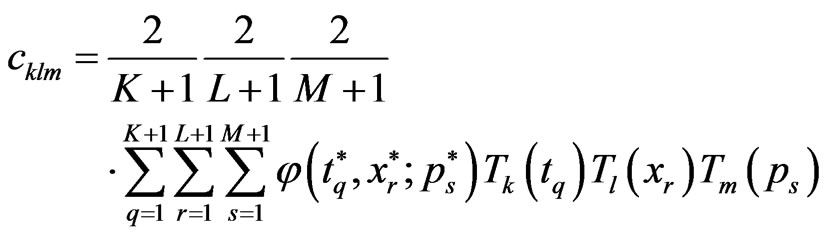 (20)
(20)
where
The Chebyshev approximation given by Equations (19), (20) can be shown to be, under rather mild conditions, an accurate polynomial approximation of  [14]. The boundary condition Chebyshev expansion coefficients
  and
and  are obtained by using the twodimensional version of Equations (19), (20) with the known functions
  and
and . Clearly, if
  then all coefficients
  and
and  must be zero. From Equations (3) and (18) we obtain the relations
 (21)
(21)
Since 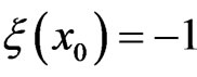 and
and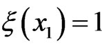 , we use Tl(−1) = (−1)l
and Tl(−1) = 1 to implement the two boundary conditions at the highest modal numbers of the spatial Chebyshev coefficients;
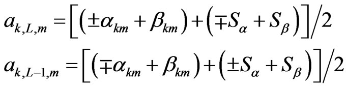 (22)
(22)
for L being even (upper sign) or odd (lower sign), respectively, with
 (23)
(23)
The Chebyshev coefficients  in Equations (8) and (13), for the initial condition expansion, are computed by using the analytical form for
  in a two-dimensional formulation of Equations (19), (20) in physiccal and parameter space.
It should be noted that a useful simplification occurs for periodic boundary conditions, for which case  . This relation is only satisfied for even Chebyshev polynomials. Considerable computation time is thus saved by only computing coefficients
  with even values of l.
In summary, initial and boundary conditions are initially transformed into Chebyshev space by use of Equations (19), (20) in suitable dimensional forms. All subsequent computations are performed in Chebyshev space, using Equations (13) and equations for the boundary conditions of the form (23). When sufficient accuracy in the coefficients  is obtained, the solution Equation (3) is obtained in physical variables. For periodic boundary conditions, coefficients
  with l odd can be neglected.
4. Nonlinearities in Spectral Space
Nonlinear terms of the operator D are treated fully spectrally in this method, in contrast to in pseudo-spectral schemes [13], where the nonlinearities are transformed to physical space, multiplied there and then transformed back to spectral space. This procedure causes the problem of aliasing, which is avoided in the present scheme. In the GWRM, as nonlinear products are produced in spectral space, Chebyshev modes that lie outside the modal representation (K, L, M) will be truncated with associated loss of accuracy. As mentioned earlier it can be shown that truncated Chebyshev polynomials, because of their minimax properties, are the most accurate polynomial representation to this order [14].
For the sake of simplicity, we now discuss the handling of a second order nonlinearity in one-dimensional Chebyshev spectral space. Higher dimension cases are easily obtained from that of one dimension. We also omit the arguments of the Chebyshev functions, which are assumed identical.
Thus we wish to determine the coefficients  in
in
 (24)
(24)
A basic and useful relationship is the identity TmTn =  , which “linearizes” expressions containing simple products of Chebyshev polynomials. Since all variable expansions have the same number of modes within the same space (temporal, physical or parameter space), we may assume that
  in Equation (24). After some algebra, the following exact expression is determined:
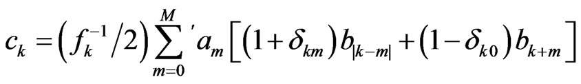 (25)
(25)
being valid for 0 ≤ k ≤ 2M. Here  for
for , and
, and  for
for . The prime on the summation sign denotes that all occurences of a zero index of a and of b should render a multiplying factor of
 . Note that only the coefficients for the employed spectral space are computed (we thus compute
  for 0 ≤ k ≤ M); other terms are truncated. The computation is best facilitated by creating a procedure that can be repeatedly called also when computing coefficients for higher order nonlinearities.
5. Solution of Algebraic Systems of Equations for Chebyshev Coefficients
The GWRM solution to an initial-value problem is found when the Chebyshev coefficients of Equation (13) are determined to sufficient accuracy. For a linear problem, the coefficients can be obtained by a simple Gaussian elimination procedure. Nonlinear differential equations, however, lead to nonlinear algebraic equations and these may be difficult to solve numerically [15]. We thus need a robust nonlinear solver that converges both globally and rapidly. Although various such methods already exist [15], we have found it rewarding to develop a new semi-implicit root solver, SIR [16], as described below.
The GWRM is well adapted for solution using iterative methods for two reasons. First, Equation (13) can be immediately cast in the fixed-point iterative form
 (26)
(26)
where the solution vector x here contains the Chebyshev coefficients  to be determined, and the vector function
  reflects the functional forms of
  and
and . Second, all iterative methods require an initial estimate of the solution vector, and if this deviates too much from the solution to be determined, numerical instability results. For the GWRM, the coefficients that correspond to the solution for the entire time domain (the roots of the equations) may deviate strongly from the coefficients of the initial state. One of the simplest and most frequently used solvers, Newton’s method, features a fairly limited domain of convergence [15,17,18], however. Because the initial guess in the case of the GWRM is precisely the initial condition, there always remains the possibility to reduce the solution time interval
 , for example by using subdomains as described below, so that the solution Chebyshev coefficients become sufficiently close to the initial Chebyshev coefficients. This, incidentally, shows that a GWRM formulation of a well posed initialvalue problem in principle always will lead to a solution, although we do not prove this rigorously at present.
Newton’s method is usually globally improved by the addition of line-search methods, in which the iteration step size is decided from the minima of the function, the roots of which are to be determined. Unfortunately, these methods may land on spurious solutions, corresponding to local minima rather than to true zeroes of the function. We have thus developed the semi-implicit root solver (SIR), being an iterative method for globally convergent solution of nonlinear equations and systems of nonlinear equations. By “global” is here meant that correct global solutions are usually (but not always) found, having the the new feature that they are never local, non-zero minima. It is shown in [16] using a set of test problems, that global convergence is at least as good as for Newton-like line-search methods. Convergence is quasi-monotonous and approaches second order in the proximity of the real roots. The algorithm is related to semi-implicit methods, earlier being applied to partial differential equations. We have shown that the Newton-Raphson and Newton methods are limiting cases of the method. This relationship enables efficient solution of the Jacobian matrix equations at each iteration. The degrees of freedom introduced by the semi-implicit parameters are used to control convergence.
Details of SIR are given in [16]; we here only briefly describe the basic formulation. Instead of direct iteration, using Equation (26), the semi-implicit method leads instead to the problem of finding the roots to the N equations
 (27)
(27)
or, in matrix form
 (28)
(28)
The system (28) has the same solutions as the original system, but contains free parameters in the form of the components  of the matrix A. These parameters are determined by specifying the values of
 , the gradients of the hypersurfaces
 . The latter gradients control global, quasi-monotonous and superlinear convergence. In SIR,
  for all m ≠ n, whereas
  is finite and is chosen to produce limited step lengths and quasi-monotonous convergence; it usually approaches zero after some initial iterations. Since Newton’s method is a limiting case of the present method, namely when all
 , rapid second order convergence is generally approached after some iteration steps. The relationship to Newton’s method fortunately leads to approximately similar numerical work, essentially that of solving a Jacobian matrix equation at each iteration step.
There are two aspects of the GWRM that are of particular importance for the root solver. First, the algebraic equations to be solved are polynomials of the same order as the nonlinearity of the original differential equations. For example, second order nonlinear pde’s lead to the solution of a system of second order polynomial equations by SIR. Since a large class of problems in physics, formulated as pde’s, feature second (or third) order nonlinearities, there is a potential to device more efficient versions of SIR where this fact has been utilized. Second, most of the computational time in SIR, when applied to the GWRM, is not spent on matrix equation solution, but rather on function evaluation. If the functions  are formulated and evaluated more economically, computational efficency may be improved.
We conclude this section by stating that the SIR algorithm has turned out to be robust and well suited for all GWRM applications tried to date. Further development would focus on the possibility to enhance SIR efficiency by economizing the handling and evaluation of the polynomial Equation (13).
6. Temporal and Spatial Subdomains
The number of arithmetical operations due to matrix inversion typically feature a cubic dependence on the number of unknowns. The root solver, applied to Equation (13), thus may dominate computational time. Applied to Equation (3), straightforward application of GWRM and SIR would require about  operations for each iteration when solving Equation (13). Using LU decomposition rather than matrix inversion, the number of operations is reduced to
  [15]. As shown in the examples of the next section, this may often be an acceptable amount of work.
In more complex calculations, efficiency requires the temporal and spatial domains to be separated into subdomains. This enables a linear rather than a cubic dependence of efficiency on, for example, the number of spatial modes applied to the entire domain, given that the number of subdomains is proportional to L. Assume that the temporal and spatial domains are divided into Nt and Nx subdomains, respectively. This reduces  operations to
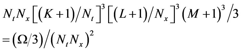
operations when solving a particular problem, assuming that the same total number of modes are sufficient in both cases. As an example, for K = L = 11, M = 2 and Nt = Nx = 3 there would be a reduction from about 2.7 × 10⁷ to 3.3 × 10⁵ operations Additionally it should be noted that the functions  in SIR will become substantially less complex when subdomains are used, with resulting reduced computational effort.
Temporal and spatial subdomains must be implemented differently. For the temporal domain the procedure can be more straightforward. As initial condition for each domain, we here simply use the end state of the previous one. It should be recalled, however, that a GWRM (as well as any WRM) solution is not per se a Chebyshev approximation of the true solution, but rather stems from a minimization of the residual, including information concerning the differential formulation of the problem, over the solution domain. Simple averaging (by using a few modes) over regions with strong temporal gradients is thus likely to produce large errors, due to the poorly approximated differential character of the problem. As will be shown, a preferred solution is to use an adaptive scheme, which uses few modes by default in each subdomain, but increases this number whenever accuracy so requires. Furthermore, the use of temporal subdomains is beneficial for SIR convergence, since the initial condition for each domain will be closer to the final solution than what would be the case using a single temporal domain instead.
Spatial subdomains must be treated in another fashion. The reason is that boundary conditions are usually only known at the exterior, rather than at interior, boundaries. A computation is not conveniently progressed successsively through a sequence of spatial subdomains, as for temporal subdomains. Instead the boundary conditions are imposed on the outermost spatial subdomains, and the subdomains are connected at interior boundaries through continuity conditions. The functions themselves and their first derivatives are continuous across each subdomain (interior) boundary. All spatial subdomains are updated in parallel at each solution iteration. Computationally, the choice of procedure is a nontrivial task. Due to the large coefficients, appearing in higher order derivatives (see Equations (16), (17)), derivative matching is sensitive to small errors and numerical instability may result. Instead we have found that a ”handshaking procedure” where the functions are allowed to overlap into neighbouring domains, and are doubly connected, yields improved stability over derivative matching.
Subdomains may also be introduced into the physical parameter domain, if desired. The final set of piece-wise solutions (3) may easily be displayed using Heaviside functions as global solutions. Should a single global, semi-analytic solution be desired, a Chebyshev approximation covering all subdomains may be carried out at the end of the computation. Concluding, the use of temporal, spatial and parameter subdomains offers substantial potential for reducing GWRM computational time, because of the possible transition from cubic to near linear dependence on the number of modes. Details of subdomain applications will be published separately.
7. Example Applications of the GWRM
We now turn to the important questions of accuracy and efficiency. In this section, the GWRM is compared by example to other methods for solving partial differential equations, that use time discretization in the form of finite differencing. Even though the GWRM generates semi-analytic solutions, it must be comparable to these standard methods with regards to accuracy and efficiency to be of practical use.
To study performance when applied to nonlinear problems, a stiff ordinary differential equations is first solved. Adaptive, temporal subdomains are here showed to provide high accuracy and efficiency.
As a second example the nonlinear, 1D viscous Burger equation is solved. It features a shock-like structure near the boundary. It is shown that GWRM accuracy is comparable to that of the (explicit) Lax-Wendroff and (implicit) Crank-Nicolson schemes for a similar number of floating operations.
Next we study a problem with two strongly separated time scales. For the wave equations without and with a forcing term, the GWRM turns out to be considerably more efficient than both the Lax-Wendroff and the CrankNicolson solution methods when tracing the dynamics of the slower time scale.
The GWRM is finally applied to the demanding problems of solving the linearized systems of ideal and resistive magnetohydrodynamic (MHD) equations. Similar problems are of key importance when studying the stability of magnetically confined plasmas for purposes of controlled thermonuclear fusion.
7.1. Introductory Example: The Match Equation
When a match is lighted, the flame grows rapidly until the oxygen it consumes is balanced by the oxygen that comes through the surface of the ball of flame. A simple model for the flame propagation in terms of the ball radius  is
is
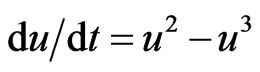 (29)
(29)
with
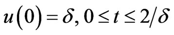 . (30)
For small values of  this problem becomes very stiff through the presence of a ramp at
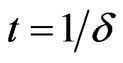 , representing the explosive growth of the ball towards its steady state size [19]. We have solved this problem by using Equation (25), transforming it to the form of Equation (2), yielding a set of equations corresponding to Equation (13) in which spatial and parameter modes are omitted. A solution with
  is presented in Figure 2. We have imposed an accuracy of
  = 1.0 × 10⁻⁴. The GWRM solution is compared with the exact solution to Equations (29), (30);
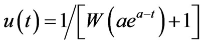 (31)
(31)
where  and W is the Lambert W function.
Clearly, for this small value of  the ramp is very distinct and hard to resolve. Consequently, explicit finite difference methods will need extremely small time steps to resolve this problem. An optimised Matlab solution to the problem uses implicit methods that may reduce the computational effort to about 100 time steps, taking a few seconds on a tabletop computer. The GWRM solution in Figure 2 uses 69 temporal domains and takes just about the same amount of computational time, but has the additional feature to provide analytical approximations to the solution in each domain. These may be of particular interest in the ramp region. For efficiency, the temporal domain length has been automatically adapted as follows. Since
 , we obtain the criterion for accuracy
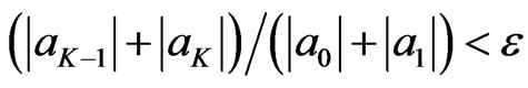 .
.
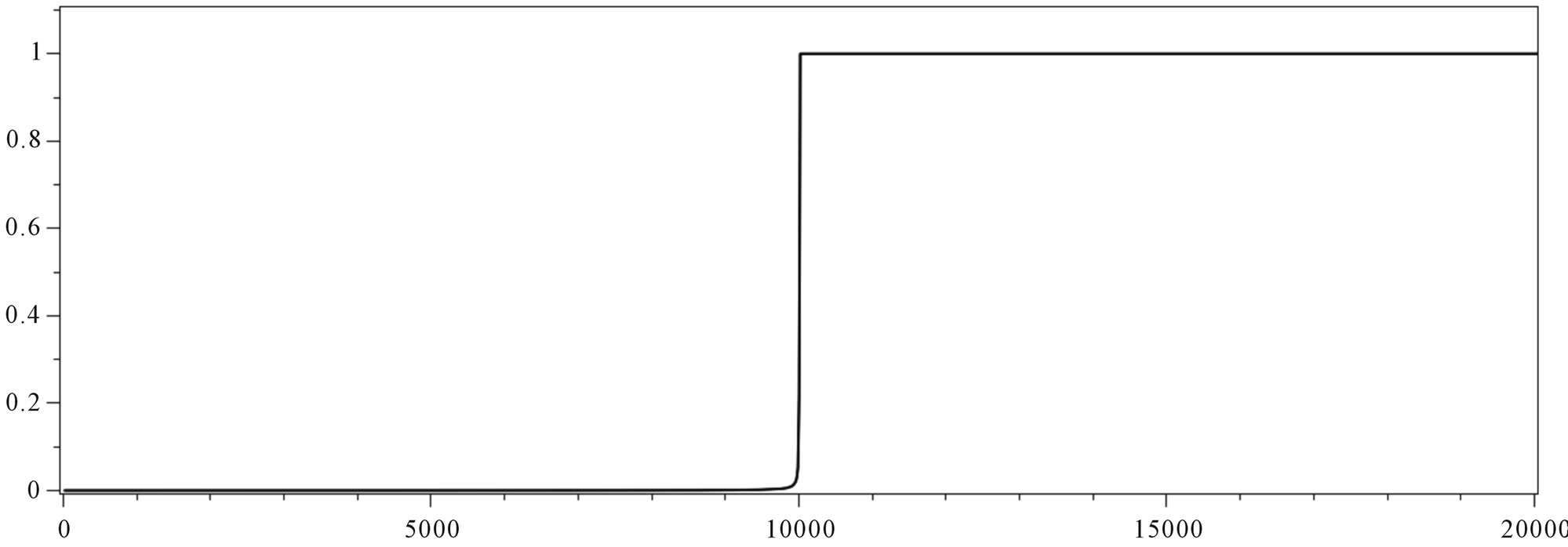
In performing the computation, a default of 10 time subdomains is assumed and K = 6 is used throughout. If the accuracy criterion is satisfied, the subdomain length is doubled at the next domain, and if not it is halved. In the latter case, the calculation is repeated for the same subdomain until the accuracy criterion is satisfied. This goes on as the calculation proceeds in time until near the endpoint, where the subdomain length is adjusted to land exactly on the predefined upper time limit. Due to the stiffness of the problem in Figure 2, the subdomains are concentrated near t = 1.0 × 10⁴ where the subdomain length may be as small as about 2 time units. The automatic extension of the subdomain length in smoother regions saves considerable computational time; at the end of the calculation the subdomain length is several thousand time units.
The essential information provided by the computations of Figure 2 is in the transformation from the plateau u = 0 to the plateau u = 1 at t = 1.0 × 10⁴. Perhaps we are willing to sacrify accurate details of the transition region, and would be satisfied with a global GWRM solution that only approximately models the transition, using only a few modes. As discussed earlier, GWRM solutions are not identical to Cheyshev approximations of the true solutions, but also mirrors the effect that results from the differential formulation of the problem. In other words—an implicit formulation of a function as a differential equation plus initial and boundary conditions will render approximate solutions that are, in some sense, imprints of the formulation. This imprint will, of course, diminish as the true solution is approached. We note that
 (a)
(a)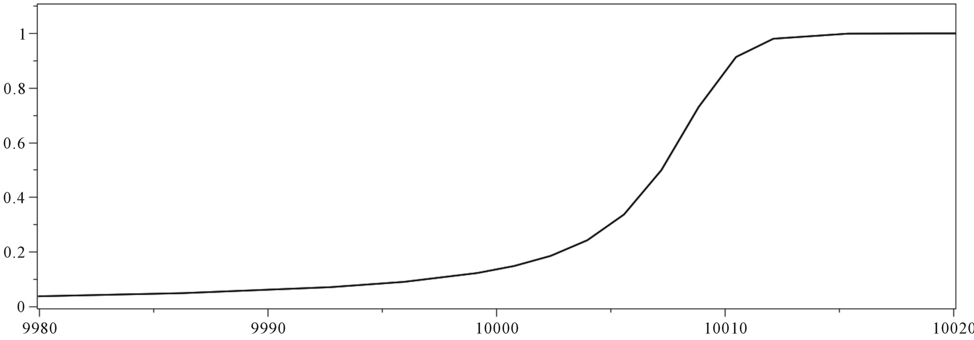 (b)
(b) (c)
(c)
Figure 2. (a) Solution to the match equation (29), with δ = 0.0001, K = 6, ε = 0.0001, using initial subdomain length of (2/δ)/10; (b) As (a), with ramp region at t = 1/δ enlarged; (c) Absolute error for the computation of (a).
in Equation (29) there are quadratic as well as cubic nonlinearities. As a result a global, low mode approximation of the solution is not trivially obtainable. The transition region needs a certain amount of resolution to “tie” with the solutions at lower and higher times t. This is an interesting topic for future studies.
In summary, a stiff ordinary differential equation has been solved to high accuracy using the GWRM. Due to use of automatic domain length adaption, high efficiency is also obtained, comparing well with highly optimised Matlab routines for implicit finite difference methods.
7.2. Accuracy; Burger’s Equation
Burger’s equation is of particular interest since it is nonlinear and contains two time scales as a result of the competition between convection and diffusion. The onedimensional Burger partial differential equation
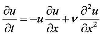 (32)
(32)
Thus contains essential physics, such as convective nonlinearities and dissipation, expected to be encountered also in more complex problems of fluid mechanics and MHD. Here  denotes (kinematic) viscosity. Since this equation has an analytical solution, it provides excellent benchmarking.
7.2.1. Exact Solution of Burger’s Equation
The exact solution to Equation (32) is found by first introducing the Cole-Hopf transformation [6]
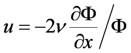 (33)
(33)
to produce a standard diffusion equation in  and then by using the Fourier method. The result, for the boundary conditions
  is
is
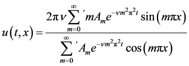 (34)
(34)
with coefficients
 , (35)
where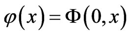 . As an example, the initial condition
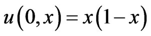 (36)
(36)
results in
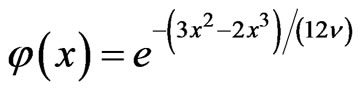 . (37)
It should be noted that the sums of the exact solution Equation (34) may need to be carried out over a large number of terms for sufficient accuracy, because of the poor convergence at low viscosity. As  at least 100 terms are required to compute a solution that gives a reasonably accurate solution near t = 0. Furthermore, in contrast to polynomials or Chebyshev polynomials, the exponential and trigonometrical functions of Equation (34) are costly to evaluate numerically. This is one example of an exact solution that is of limited practical use.
The most challenging aspect of the Burger equation, from the modelling point of view, is the shock-like structure that evolves for weak dissipation. The associated gradients are often difficult to resolve in spectral representations. Highly accurate modelling may require a high number of Chebyshev modes. The case we study develops a strong gradient near the boundary x = 1, and is representative of the gradients in, for example, edge pressure or temperature, encountered in magnetohydrodynamic computations in fusion plasma physics modelling. The structure may also appear when modelling localized resistive instabilities in tokamak and reversedfield pinch magnetic fusion configurations. It is desired that the GWRM should be able to resolve these structures for limited values of mode numbers. To see the difference as compared to standard modelling, we make comparisons to solutions obtained from the standard explicit Lax-Wendroff and implicit Crank-Nicolson finite difference schemes for partial differential equations [15].
7.2.2. GWRM Solution of Burger’s Equation
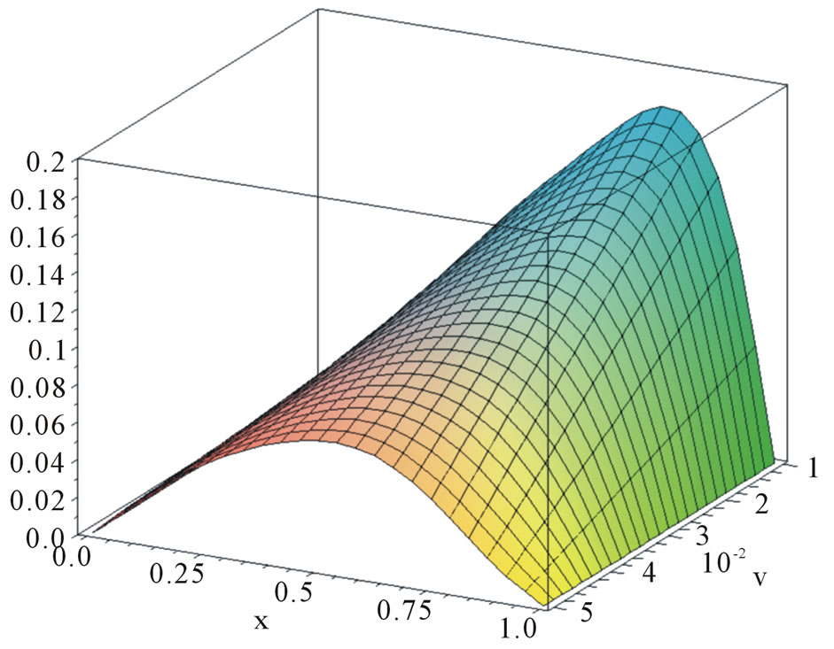
In Figure 3(a), the GWRM solution of Burger’s equation for boundary conditions  and initial condition
  is shown. Nine temporal (K = 8), eleven spatial (L = 10) and three parameter (viscosity) modes (M = 2) were required to obtain an error better than 1% after 7 iterations. The solution is valid within the domains given by
 ,
,  and
and , and is displayed for fixed t = 2.5. Note that the solution was attained for all viscosities in the given range in a single computation. It is seen that a sharp gradient builds up near the edge, being most profound for small values of viscosity. If the number of temporal or spatial modes are reduced somewhat, the same accuracy is retained everywhere except for near the edge x = 1. Since the “exact” Cole-Hopf solution converges slowly at these low values of
 , the obtained GWRM semi-analytical solution is actually computationally more economical to use in applications.
To enable comparisons with explicit and implicit finite difference partial differential equation solvers, we will now fix viscosity to  and compute the solutions as functions of t and x. The Burger equation, defined as above but now using t1 = 10, is solved using all GWRM, explicit Lax-Wendroff, and implicit Crank-Nicolson methods [15]. The latter two schemes are accurate to second order in both time and space.
For the GWRM solution, two spatial subdomains with internal boundary at x = 0.75 are used. A similar result would be obtained using only one spatial domain with slightly higher number of spatial modes. With mode numbers K = 9, L = 7 an absolute global accuracy of 0.001 is obtained after 10 iterations, with a tolerance of 1.0 × 10⁻⁶ for the coefficient values. Results are displayed in Figures 3(b) and (c). The peak near t = 0 in Figure 3(c) is due to the poor convergence of the exact solution of which 60 terms are used.
7.2.3. Lax-Wendroff Explicit Finite Difference Solution of Burger’s Equation
We now turn to solution of the Burger equation using finite difference methods. Accurate solutions are not straightforwardly obtained because of the strong edge gradient. Let us estimate the spatial step length required for a global error  = 0.001. A second order estimate of the mid-point error resulting from finite spatial differencing with spacing
  is
is
 (38)
(38)
where a prime denotes spatial differentiation. From the exact solution it is found that  = 20.3 at (t, x) = (2.05, 0.94). A maximum global error of δ = 0.001 thus requires
  < 0.02.
The Lax-Wendroff finite difference scheme is widely used because of its reliability and because it is accurate to second order in both time and space. Since it is explicit, the maximum time step becomes limited, however. A von Neumann analysis of the Lax-Wendroff method applied to the Burger equation (32) features the limiting cases of strong convection or strong diffusion. When convection dominates the CFL condition , where
  is a characteristic fluid velocity, results. This condition characterises the required causality on the solution grid for hyperbolic problems. When the diffusion term dominates, the problem is parabolic and the time step is limited to
 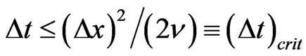 by causality. Computations show that the latter criterion is the more relevant one for the present Burger problem.
Recall that accuracy requires  < 0.02 according to Equatiom (38). This is in reasonable agreement with the value
  ≤ 1/70, that was found numerically. For
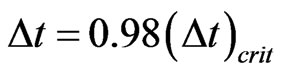 , the number of time steps becomes 1000 for the given accuracy. The error of a Lax-Wendroff computation is shown in Figure 3(d). High accuracy is obtained everywhere except near the maximum spatial gradient. Using Maple 12 on the same platform for both methods, the Lax-Wendroff method needs 50% less time than the GWRM. It is thus somewhat more accurate for the same number of computational operations in this case. Note, however, that the discussion in Section 3.1 shows that for the case of a single spatial domain, the boundary conditions would be periodical (or homogeneous) in which case odd spatial mode numbers can be omitted and an eight-fold gain in efficiency would be attainable. The GWRM solution has also the advantage of being in analytic form whereas the Lax-Wendroff solution is purely numeric.
7.2.4. Crank-Nicolson Implicit Finite Difference Solution of Burger’s Equation
Next, we solve the Burger equation using the CrankNicolson method. This scheme allows for arbitrarily large time steps by using an implicit approach where the functional values are determined both at the previous and present time steps. On the spatial scale, the resolution ≤ 1/70 is, however, still needed to obtain a global accuracy of 0.001. To avoid costly matrix inversion at each time step, due to the implicit finite difference formulation, a tridiagonal matrix solution procedure has been developed [15] that radically speeds up the calculations for linear equations. To be able to use this scheme for the nonlinear Burger equation, we advanced the linear diffusive term using the standard Crank-Nicolson method, but advanced the nonlinear convective term explicitly. As a result, a von Neumann analysis shows that the time step is no longer unrestricted, but must obey the relation
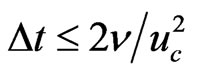 . Note that this relation is independent of
 .
.
For a time step  = 1/500 and with
  = 1/70, an accuracy of 0.001 was achieved for the Burger equation, as shown in Figure 3(e). The computer time used was about half that of the Lax-Wendroff method. For general nonlinear problems, when a linear higher order term that can be advanced explicitly does not exist, this method may be less accurate however. The reason is that, for making use of efficient tridiagonal matrix solving, the differential equation should be time linearized, which introduces errors.
7.2.5. Conclusions on Solution of Burger’s Equation
Interestingly, we have found that the analytical GWRM solution of Burger’s equation is more economic than the “exact” Cole-Hopf solution for use in applications at low values of  for given accuracy, due to the poor convergence of the latter. Although the GWRM is primarily intended for computing long time behaviour of complex problems with several time scales, it can thus be used for accurate solution of stiff problems. For the case of Burger’s equation, the GWRM was nearly as efficient as the Lax-Wendroff and Crank-Nicolson schemes for given accuracy. For nonlinear problems, where all terms must be advanced implicitly, the Crank-Nicolson method is expected to compare less favourably with the GWRM either due to reduced efficiency when solving a nonlinear system of equations at each iteration or due to reduced accuracy if nonlinear terms are time linearized. Improved GWRM efficiency is also expected for problems with
 (a)
(a)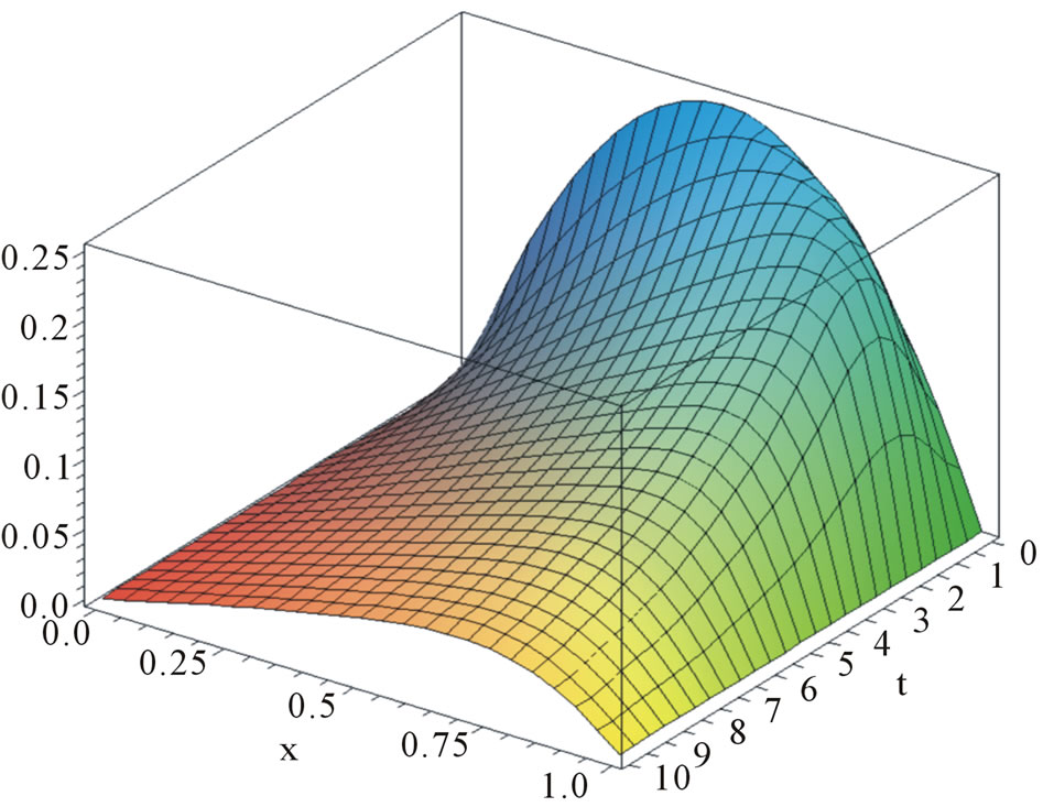 (b)
(b)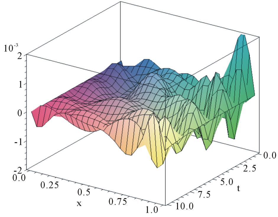 (c)
(c)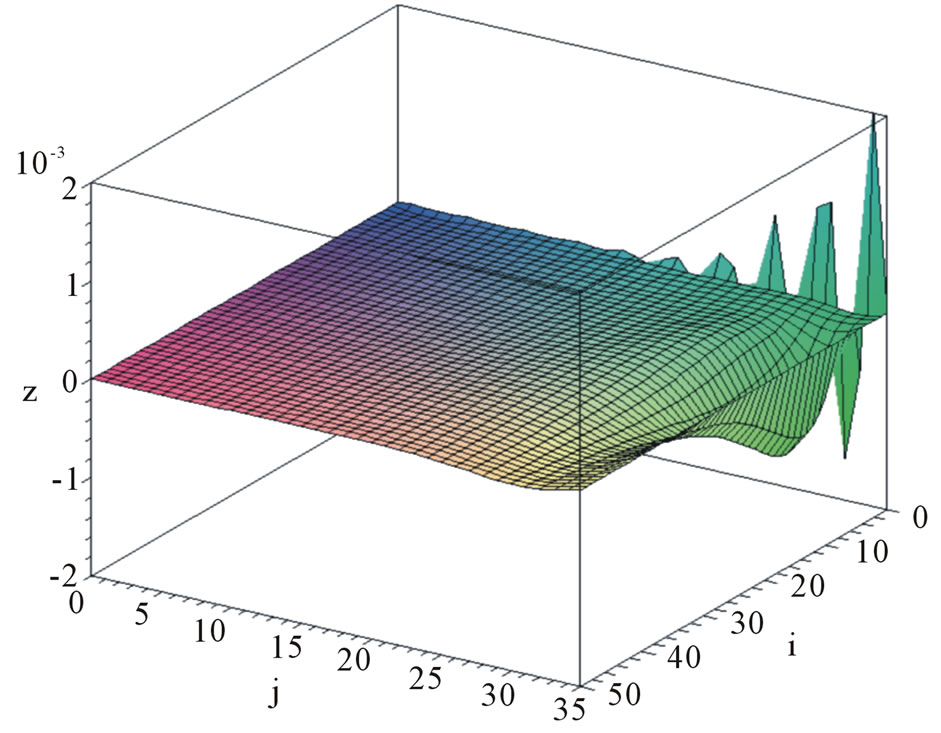 (d)
(d)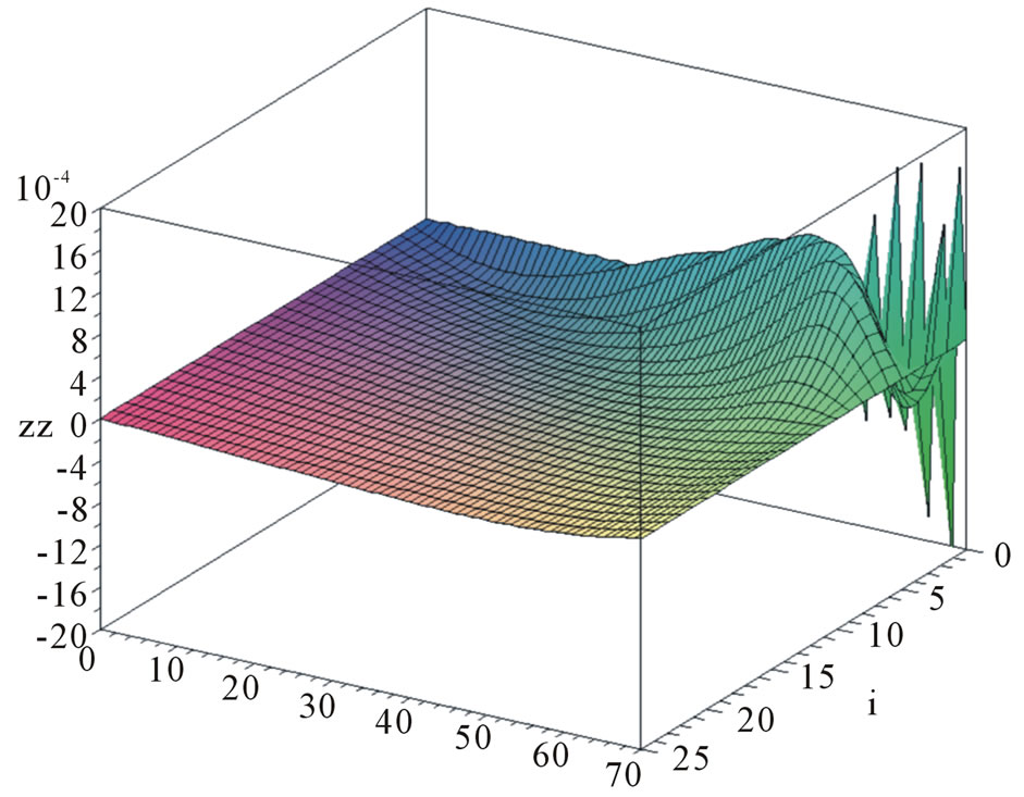 (e)
(e)
Figure 3. (a) GWRM solution of Burger’s Equation (32) with initial condition φ(x) = x(1 − x), boundary condition u(t, 0) = u(t, 1) = 0, shown versus x and ν at time t = 2.5. K = 8, L = 10, and M = 2; (b) GWRM solution of Equation (32) with φ(x) = x(1 − x) and u(t, 0) = u(t, 1) = 0, for ν = 0.01. Two spatial subdomains are used, with internal boundary at x = 0.8, and K = 9, L = 7; (c) Difference between the exact solution of Burger’s equation (first 60 terms of Equation (34)), and the GWRM solution; (d) Difference between the exact and the Lax-Wendroff solutions of Burger’s equation, for ν = 0.01. Here 1000 time steps were used, and ∆x = 1/70. Only each 20th time step and each 2nd spatial step are shown; (e) Difference between the exact and the Crank-Nicolson solutions of Burger’s equation, for ν = 0.01. Here 500 time steps were used, and ∆x = 1/70.
periodic boundary conditions. The GWRM has the additional advantage of providing approximate, analytic solutions.
7.3. Efficiency: The Forced Wave Equation
Problems in physics often feature multiple time scales, whereas it may be of main interest to follow the dynamoics of the slowest time scale. Efficient partial differential equation solvers therefore must be able to employ long time steps, retaining stability and sufficient accuracy. By omitting resolution of the finer time scales, improved efficiency and the possibility to study complex systems are expected. As a test problem, we choose a wave equation with a forcing (source) term, also called the inhomogeneous wave equation:
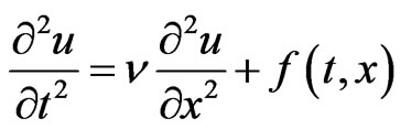 (39)
(39)
with boundary and initial conditions

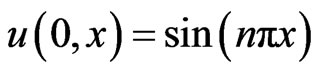
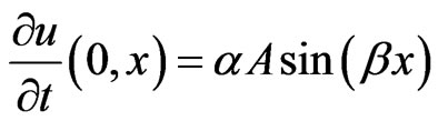
Here A, n,  ,
,  and
and  are free parameters, and
 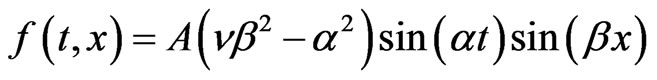 is the forcing function. The exact solution is
 (40)
(40)
for , with m an integer. This problem has the separate system and forcing function time scales
  and
and . Using the parameter value
 ,
,  ,
,  ,
,  and
and , the ratio of these time scales becomes
 . Thus the forcing term in (40) has here introduced a time scale much longer than that of the “unperturbed” system.
7.3.1. GWRM Solution of the Forced Wave Equation
We now wish to solve Equation (39) using all GWRM, Lax-Wendroff and Crank-Nicolson methods. The problem is thus posed as a set of two first order partial differential equations:
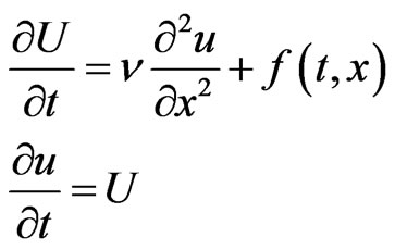 (41)
(41)
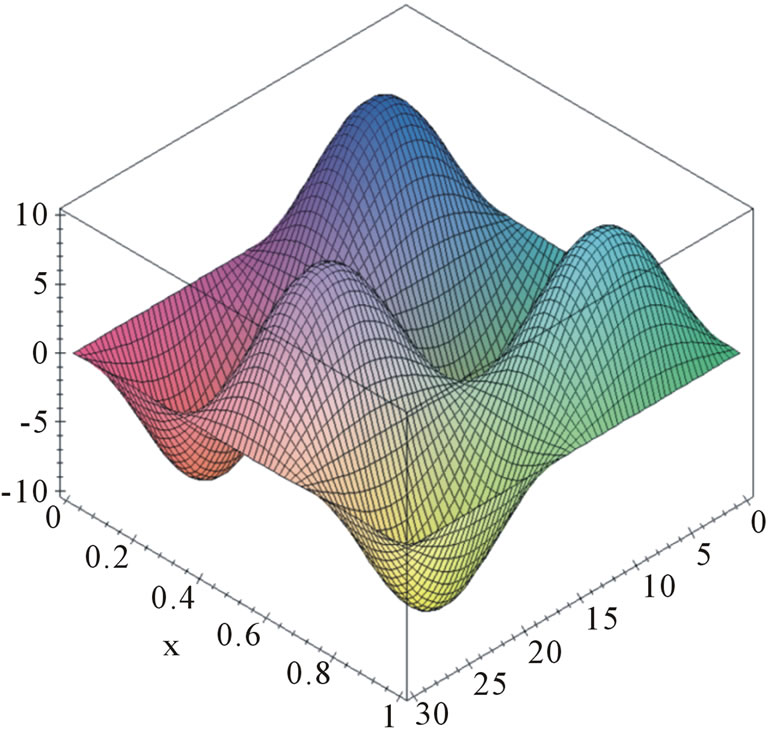
with boundary and initial conditions corresponding to those of Equation (39). The GWRM solution, using one spatial domain with K = 6 and L = 8, is rapidly obtained within a single iteration with a tolerance of 1.0 × 10⁻⁶ for the coefficient values. It is displayed in Figure 4(a). The solution behaves as desired; it averages over the faster (system) time scale and follows the slower (forced) time scale in an averaging sense. This is shown in more detail in Figure 4(b), where the temporal evolutions of both the exact and the GWRM solutions are shown jointly for fixed x. The averaging character of the solution remains at least for all values K ≤ 20.
7.3.2. Lax-Wendroff Explicit Finite Difference Solution of the Forced Wave Equation
We now turn to finite difference solution of Equation (39) using the Lax-Wendroff method. Being an explicit method, it must obey the CFL condition, which for this case becomes . We find that sufficient accuracy is obtained for
  ≤ 1/30. Thus the maximum allowed time step is 1/30, and the number of time steps becomes 900 for the domain
 . The calculation requires about ten times more computer time than the GWRM. It can be seen in Figure 4(c) that the solution initially traces the exact solution, but thereafter follows the slower time scale. The solution appears not to average as accurately as the GWRM over the fast time scale.
7.3.3. Crank-Nicolson Implicit Finite Difference Solution of the Forced Wave Equation
The Crank-Nicolson method, being implicit, has no time step restriction and no amplitude dissipation and would perhaps intuitively be well suited for the present problem. Additionally, to avoid time-consuming large matrix equations, the so-called Generalized Thomas algorithm [6] uses a block-tridiagonal matrix algorithm that substantially speeds up the calculations at each time step. If the associated sub-matrix equations are solved for, rather than computing inverse matrices, a gain from Gauss elimination O((MN)3/3) operations to O(5M3N/3) operations is possible, that is the speed gain factor becomes N2/5. Here the number of equations M = 2 and the number of spatial nodes N = 30. The handling of a number of sub-matrix equations, required at each time step, is still limiting performance however. With  = 1/30, temporal resolution requires at least 50 time steps. Using matrix inversion, the corresponding computation is about three times slower than Lax-Wendroff and thus about 30 times slower than that of the GWRM. A speed gain of a factor three is expected by solving the sub-matrix equations rather than determining inverse matrices, but the GWRM remains considerable faster. It should be noted that the sub-matrices used in the Thomas algorithm are here only 2 × 2 in size. Thus negligible time is spent in matrix inversion; it is rather the extensive use of matrix manipulations in the algorithm that affects efficiency. The solution is shown in Figure 4(d) and in Figure 4(e) the solution is Chebyshev interpolated at x = 0.2 to
 (a)
(a)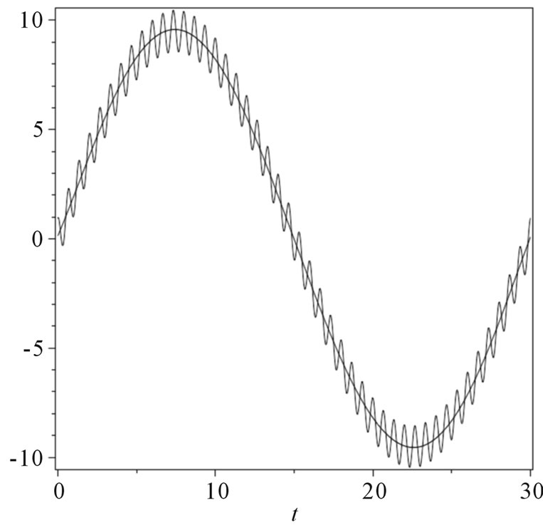 (b)
(b)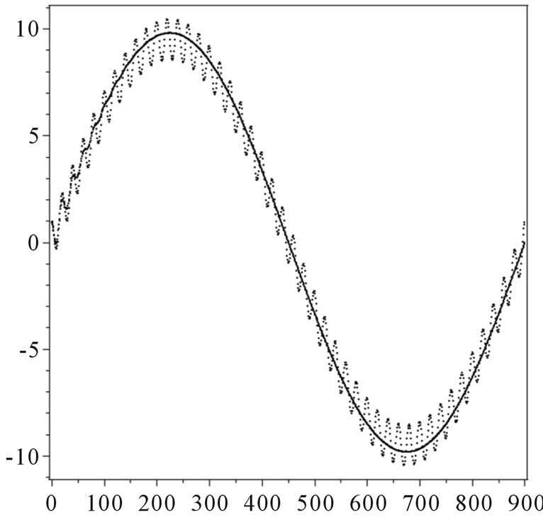 (c)
(c)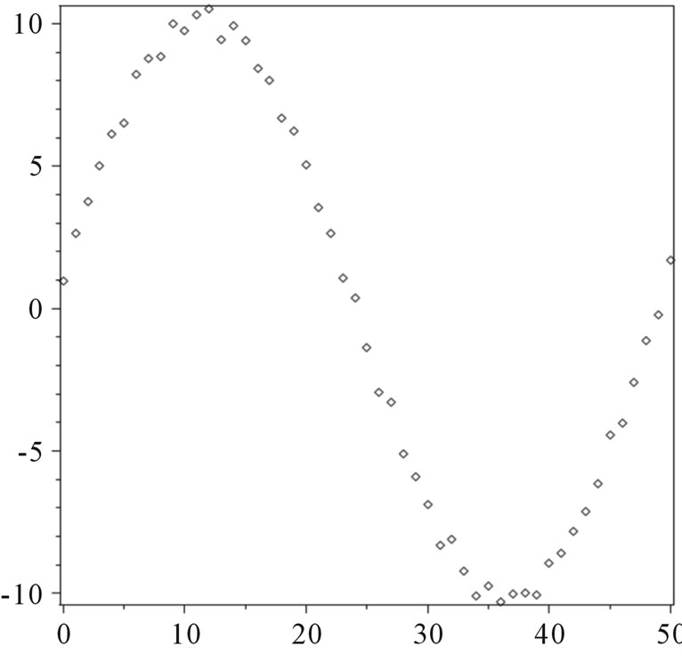 (d)
(d)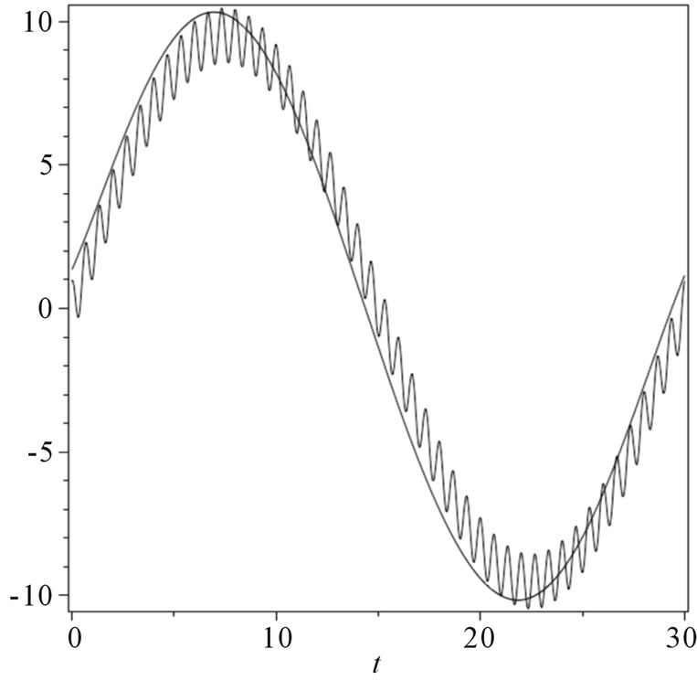 (e)
(e)
Figure 4. (a) GWRM solution of the forced wave Equation (39), using a single spatial domain, with K = 6 and L = 8; (b) GWRM temporal evolution of the forced wave Equation (39) for x = 0.2 (smooth curve) as compared to exact solution (oscillatory curve); (c) Lax-Wendroff temporal evolution of the forced wave Equation (39) for x = 0.2 (smooth curve) as compared to exact solution (oscillatory curve). Here 900 time steps are used, and ∆x = 1/30; (d) Crank-Nicolson temporal evolution of the forced wave equation (39) for x = 0.2. 50 time steps were used with ∆x = 1/30; (e) Chebyshev interpolated solution of (d) as compared to exact solution (oscillatory curve).
facilitate a comparison with the exact solution. The Crank-Nicolson solution strives to follow the exact solution, and does not accurately average over the fast time scale.
7.3.4. Conclusions on the Forced Wave Equation
It was found that the GWRM is well suited for long time scale solution of the wave equation test problem, which features both a slow and a fast time scale. For suitable mode parameters, it traces the slower dynamics using substantially less computational time than the LaxWendroff and Crank-Nicolson schemes. An important factor, contributing to the efficiency, is that whereas the Lax-Wendroff and Crank-Nicolson schemes must solve two first order Equations (41) representing the second order wave equation, the GWRM integrates both these equations formally in spectral space into one equation before the coefficient solver is launched. If results are sought for longer times, temporal subdomains are preferably used for the GRWM, to guarantee constant computational effort per problem time unit. For problems with wider separation of the time scales, the GWRM will be an increasingly advantageous method as compared to the Lax-Wendroff scheme since the latter must follow the faster time scale. It may also be noted that the GWRM averages more accurately over the fast time scale oscillations than the finite difference methods. This is a subject that deserves further attention.
This forced wave equation example featured an imposed, periodic, time scale that was longer than the system time scale. How will the GWRM perform when the imposed time scale is shorter than that of the system? At present it appears difficult to adequately handle such problems using the GWRM. A major complication is that, for efficiency, the number of modes used in the calculation would not adequately resolve the forcing function, so that the problem would not be well defined for the GWRM. This is a subject for further investigation. As seen in the case of the Burger equation, and as seen in the resistive MHD computation below, multiple time scales may also be inherent in the systems we are modelling.
7.4. Magnetohydrodynamic (MHD) Stability-Large System of Initial-Value pde’s
We now turn to applications of the GWRM to more advanced research problems featuring large sets of coupled pde’s. In fusion plasma physics research, the stability of magnetically confined plasmas to small perturbations is of considerable importance for plasma confinement. Stability can be studied using a combined set of nonlinear fluid and Maxwell equations, magnetohydrodynamics (MHD). The configuration must be arranged so that the plasma is completely stable to perturbations on the fastest MHD time scale—the so-called Alfvén time, being of the order fractions of microseconds. If plasma resistivity is included in the MHD model, further instabilities (milliseconds time scale) are accessible for the plasma even if it is stable on the faster time scale, and remedies should be sought also for these.
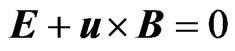
We will study the linear stability of two plasma configurations within the traditional set of MHD equations, both without (ideal MHD) and with resistivity included. By “stability” is here meant the absence of exponentially growing solutions in time. For simplicity the plasma is assumed to be surrounded by a close fitting, ideally conducting wall. It can be shown that such a wall provides maximal stability. The ideal MHD plasma equations are the continuity and force equations, Ohm’s law and the energy equation supplemented with Faraday’s and Ampere’s laws, respectively:
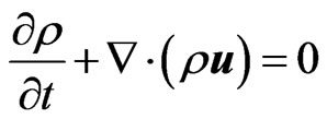
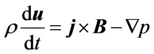
 (42)
(42)
whereas for resistive MHD, Ohm’s law becomes instead  with
with  being the resistivity. Here E and B are the electric and magnetic fields respectively, u is the fluid velocity, j is the current density, p is the kinetic pressure,
  is the mass density,
  = 5/3 is the ratio of specific heats and μ0 is the permeability in vacuum. Furthermore,
 . To determine the temporal evolution of these equations in circular cylinder geometry, they are linearized and Fourier-decomposed in the periodic coordinates
  and z. All dependent variables q of Equation (52) are assumed to be superpositions of an equilibrium term q0 and a (small) perturbation term q1. Perturbations are taken to be proportional to exp[i(kz + mθ)], where k and m denote axial and azimuthal perturbation mode numbers, respectively. Next, a non-dimensionalization is carried out using the characteristic values (denoted with index “c”) of plasma radius a, Alfvén velocity
 , with
 ,
, 
 , and
, and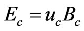 . Resulting non-dimensional equations become identical to those obtained from Equation (42) with μ0 = 1. We wish to solve for the time evolution of the perturbed terms for a given equilibrium and a specified perturbation (m, k). If these feature an exponential growth, the plasma is unstable to small perturbations for the assumed equilibrium.
7.4.1. An Ideal MHD Stability Problem
The equilibrium is here taken to be that of a simple screw pinch with constant axial magnetic field and current density and constant mass density:
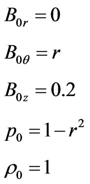 (43)
(43)
After eliminating E and j in Equation (42) there result seven complex-valued coupled partial differential equations for u1, B1 and p1 respectively as functions of the independent variables time t and cylindrical variable r. They are all written on the component form , where q1i denotes perturbed variables, to conform with the GWRM formulation of Equation (1). The seven dependent variables were all Chebyshev expanded in t, r and in resistivity
  (which was here set equal to a constant). Since the GWRM is (so far) developed for solution of real valued equations, u1, B1 and p1 are finally split up in real and imaginary parts, resulting in a system of 14 simultaneous equations to be solved by the GWRM.
Let us now discuss boundary and initial conditions. It can be shown that, in circular cylinder geometry, the following conditions must hold for m = 1 perturbations near the internal boundary r = 0:
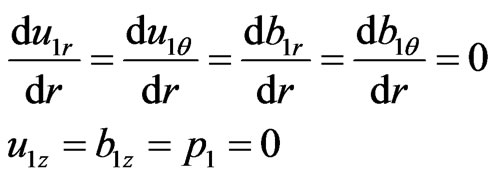 (44)
(44)
We have chosen to study m = 1 perturbations because they are often the most critical ones with respect to stability. At the outer, ideally conducting, boundary r = 1 the normal components of the fluid velocity and magnetic fields, u1r and b1r, must vanish.
The relation between the initial conditions can be chosen somewhat arbitrary. The reason is found from studies of the corresponding system of eigen-equation and is that, for unstable behaviour, a competition between modes with different number of radial nodes will take place until the fastest mode (with zero radial nodes) will dominate the behaviour. The memory of the initial perturbation is then lost. For consistency with respect to the boundary conditions we however choose the following set of initial conditions:
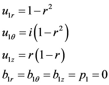 (45)
(45)
The 14 coupled pde’s we are about to solve are linearized, but nevertheless contain nonlinear terms with products between equilibrium and perturbed variables. As an example, a term proportional to  should be computed. Some care is needed in order to obtain an optimal spectral representation of this and similar terms. Due to the finiteness of the spatial spectral space, nonlinear products should always be carried out in spectral space before the “division by r problem” is treated using the procedure described below. Otherwise the lowest order spectral coefficients may be inadvertently eliminated.
Further complications thus include apparent singularities near r = 0 in terms that are divided by r. These arise due to the choice of coordinate system and must be carefully handled. For example, terms of the type  turn up when writing the perturbed Equation (42) in component form. Clearly, for m = 1 this term is finite at r = 0 due to the boundary condition
 . But it must be secured that the latter relation holds exactly to avoid singularity at r = 0. Furthermore, the equation controlling the pressure evolution contains the term
 . For the case m = 0 this is not problematic since then the internal boundary condition is
  at r = 0, but for other values of m the term requires special treatment. Similarly, the term
  causes difficulties for finite resistivity.
The following procedure was found convenient to deal with the abovementioned terms. A separate study is carried out where firstly all equations are expanded to low order as ordinary polynomials. Secondly, all internal boundary conditions (like ) are imposed. Thirdly, conditions as
  (corresponding to finite compressibility
 ) are imposed at r = 0. Fourthly, the resulting expansions near r = 0 are studied to determine whether all singularities imposed by the cylindrical coordinate system have vanished. This is indeed the case for each of the 14 MHD component equations. Thus all apparent singularities may be safely removed from the code before the coefficient Equation (13) is solved.
Removal of Chebyshev coefficients for physical terms, belonging to either of the two cases discussed above, is conveniently performed using the following procedure. The Chebyshev coefficients of the physical term to be ’washed’ are converted to coefficients of ordinary polynomials, using a procedure found in [14]. In ordinary polynomial spectral space, the lowest order spatial coefficient is then set to zero. This eliminates all spatial singularities at r = 0. Subsequently, a back transformation to Chebyshev spectral space is performed.
7.4.2. Ideal MHD Stability Problem Solved Using Both GWRM and Eigenvalue Approaches
The screw-pinch stability problem defined by Equations (42)-(45) is now solved for the perturbation (m, k) = (1, 10) using the GWRM. Parameters are K = 5, L = 5, M = 0 and five equidistant temporal domains were used. A single SIR iteration is again sufficient due to linearity in u1, b1 and p1. We will not specifically compare efficiency with other methods here, but merely note that for this case, SIR solved only 372 coupled equations for the coefficients (13). This is considerably less than the 14 × 6 × 6 = 504 equations that obtain before the boundary conditions are applied. The Chebyshev coefficients corresponding to the boundary conditions are functions of the coefficients that are solved for in SIR.
Plots of  and
and  vs t and r are given in Figures 5(a) and (b). It is seen that the equilibrium (43) results in an unstable configuration. For comparison, we have also solved the same problem using an eigenvalue approach where time dependence has been eliminated through the asymptotic assumption
  [20]. In this approach, the linearized ideal MHD equations are reduced to two simultaneous equations that are solved by a shooting procedure where the growth rate
  is guessed until the boundary conditions are satisfied. Very good correspondence between the GWRM solutions in Figure 5 and the eigenvalue solutions is found.
Of particular interest in MHD stability analysis is the value of the obtained growth rate. Assuming an exponential time behaviour for the GWRM solution during the last 10% of the temporal evolution, the normalized growth rate  = 0.83 is obtained in this highly unstable case (recall that a normalization to the Alfvén time, being less than a microsecond, is used).
The computed growth rate exactly coincides with that obtained from the eigenvalue code. Also for other perturbations (m, k) very good agreement is obtained. Considering that the two methods are radically different in idea and implementation, these results certainly confirm the applicability of the GWRM to complex systems of initial value partial differential equations. The equilibrium used in this example is easily changed within the existing computer code to more realistic cases without changing the basic GWRM performance demonstrated here.
7.4.3. A Resistive MHD Stability Problem Solved Using the GWRM
If Ohm’s law is modified to include resistivity; E + u × B = ηj, the field lines are allowed to break up and stable,
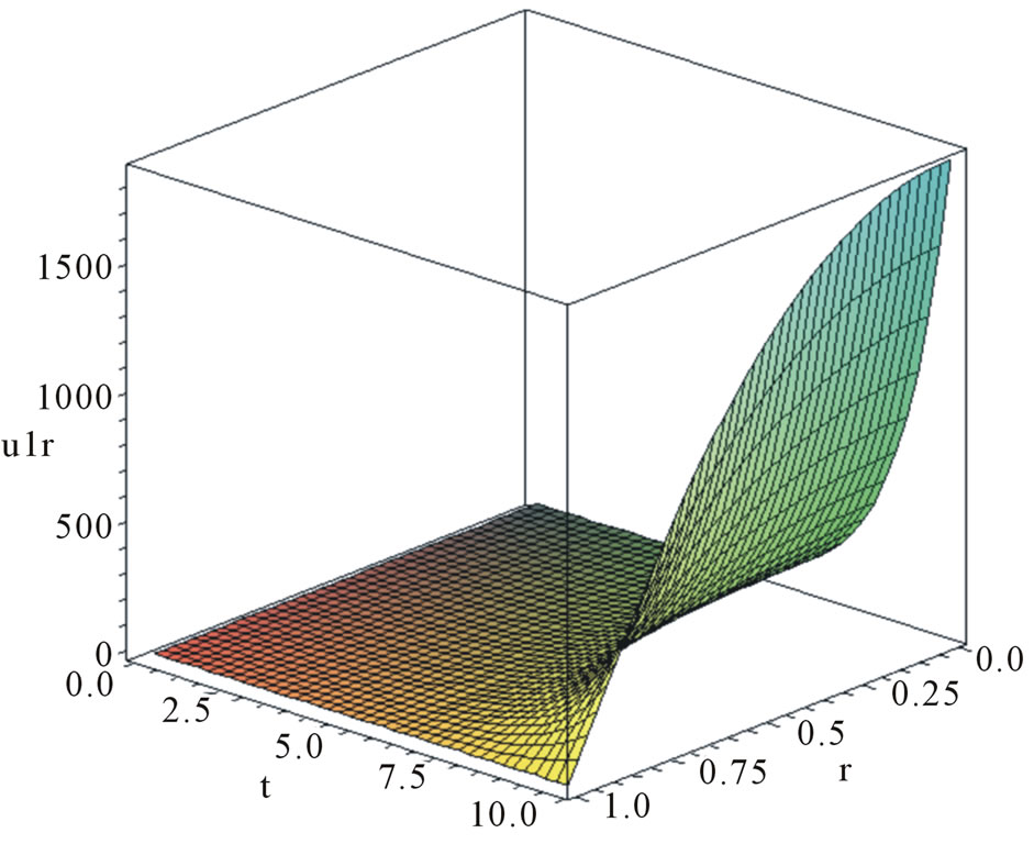 (a)
(a)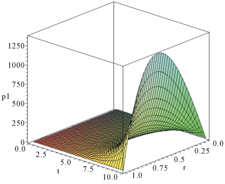 (b)
(b)
Figure 5. (a) GWRM solution obtained by solving ideal MHD Equation (42) through (45) for perturbation (m, k) = (1, 10). Parameters are K = 5, L = 5, M = 0; five equidistant temporal domains were used and a single SIR iteration. The perturbed radial plasma flow u1r is shown vs t and r; (b) As (a) but here the perturbed pressure p1 is shown vs t and r.
infinitely conducting (ideal) MHD equilibria may become resistively unstable. The finite resistivity relation is now used rather than the less realistic assumption of ideal MHD. It is easily shown that Equation (42) must now be supplemented by two new boundary conditions at r = 1 due to that the tangential component of the electric field is zero. From Ohm’s law we find that  and
and  and thus
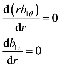 (46)
(46)
For equilibrium, we choose
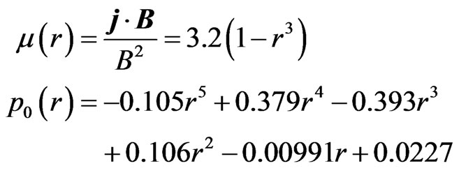 (47)
(47)
characteristic for the so-called reversed-field pinch (RFP) configuration. This equilibrium is marginally stable to ideal current and pressure driven modes. Stability is accomplished from the strong radial variation of the axial magnetic field, which provides “magnetic shear”. We further assume the perturbation (m, k) = (1, −2) which has the implication that there is a so-called resonance at at r = 0.41, near which region the plasma is particularly vulnerable to local instability (the stabilising magnetic field line bending is a minimum there). The Lundquist number  is in the range 10−4 - 10−3 in this ex- ample. The number of spectral modes are (K, L, M) = (4, 5, 1). We use 5 time intervals, a total time of 1.2 × 10³ and a single spatial domain.
Results from GWRM computations are shown in Figure 6. In particular, the temporal and spatial evolutions of the perturbed radial magnetic field, which in analytical form is
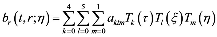 (48)
(48)
are shown. The GWRM solution also immediately enables the displayed plots of perturbed radial magnetic field and pressure as functions of plasma radius and resistivity. The growth rate of the instability (in inverse Alfvén times, assuming exponential dependence) at the end of the computation is easily obtained analytically from the temporal and parametrical dependence of the perturbed radial magnetic field as
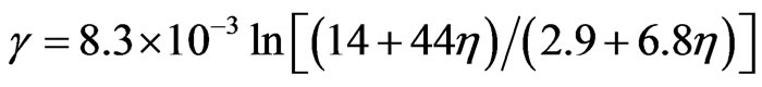 (49)
(49)
and is plotted in Figure 6(d). These results are approximate due to our choice of limited resolution (5th order)
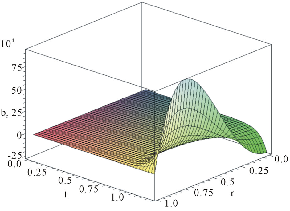 (a)
(a) (b)
(b)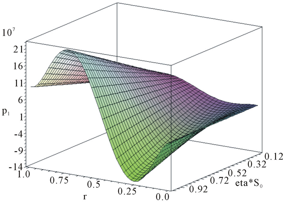 (a)
(a)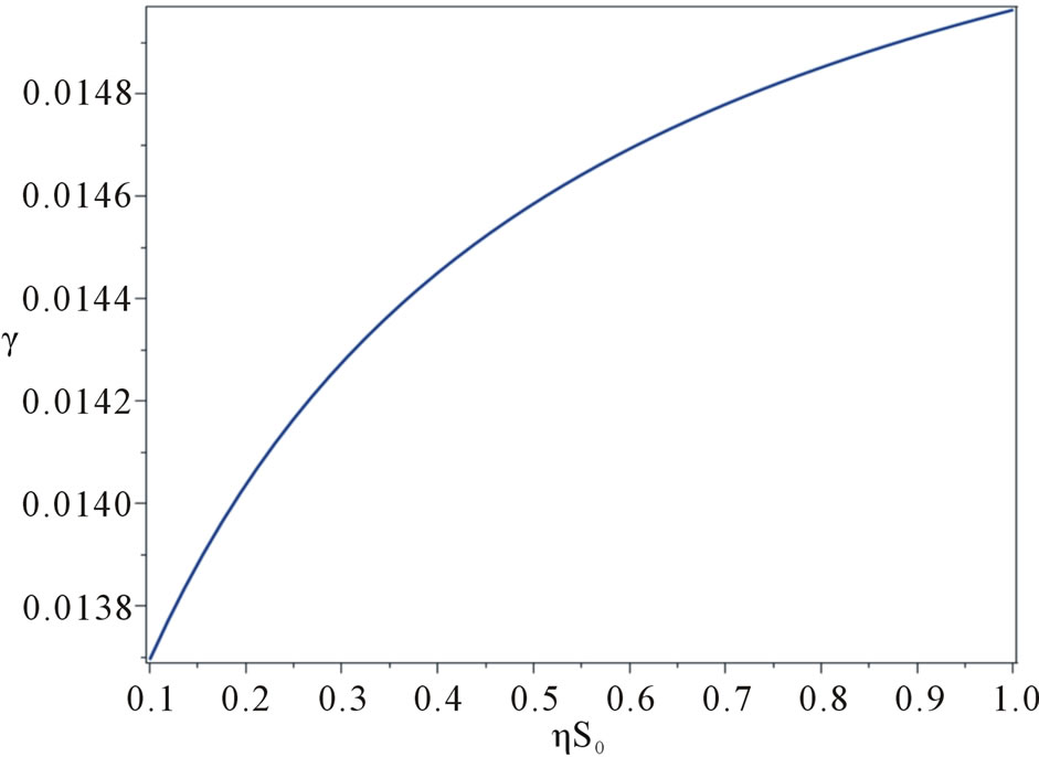 (b)
(b)
Figure 6. (a) Time evolution of perturbed radial magnetic field obtained in a resistive MHD computation using the GWRM; for details see Section 7.4.2; (b) Perturbed radial magnetic field of (a) vs r and resistivity η at end of calculation; (c) Perturbed pressure vs r and resistivity η at end of calculation of (a); (d) Growth rate of instability (in units of inverse Alfvén times) vs resistivity η at end of calculation of (a).
of the equilibrium. In ongoing work, we introduce spatial subdomains in order to provide improved resolution of both the equilibrium and the perturbations near the resonance.
7.5. Summary-Applications
We have applied the GWRM to basic linear and nonlinear initial value problems in the forms of ordinary and partial differential equations. Accuracy and efficiency have been studied by comparisons with exact solutions. Improved performance by using temporal and spatial subdomains was discussed. Comparisons with standard explicit and implicit finite difference methods showed positive results with regards to computational efficiency. Finally we have also solved advanced fusion plasma stability problems formulated within ideal and resistive magnetohydrodynamics as 14 simultaneous initial value partial differential equations. Very good agreement was here found with results from established eigenvalue methods.
Although faster computational environments than Maple exist, exact comparisons of efficiency are not essential at this stage. The examples we have given show that the efficiency and accuracy of the GWRM is comparable to that of both explicit and implicit finite difference schemes in a given environment. Further optimisation of both GWRM and finite difference codes could increase efficiency, but our ambition has been to determine whether time-spectral methods for solution of initialvalue pde’s are of interest for general use and for computations of problems in magnetohydrodynamic and fluid mechanics in particular.
8. Discussion and Conclusions
A fully spectral method for solution of initial-value ordinary or partial differential equations has been outlined. The time and parameter generalized weighted residual method, GWRM, represents all time, spatial and physical parameter domains by Chebyshev series. Thus semianalytical solutions are obtained, explicitly showing the dependence on these variables. The essence of the GWRM is its ability to transform the implicit dependencies inherent in physical laws formulated as differential equations to solutions of explicit, semi-analytical form.
The method is global and avoids time step limitations due to its acausal nature. The characteristic form of the problem (hyperbolic, elliptic or parabolic) is thus unimportant. This fact makes the method potentially applicable to a large class of problems. The spectral coefficients are determined by iterative solution of a linear or nonlinear system of algebraic equations, for which a new and efficient semi-implicit root solver (SIR) has been developed. Accuracy is explicitly controlled by the number of modes used and the number of iterations. The use of subdomains further increases efficiency and accuracy. In a separate publication, details of the use of temporal and spatial subdomains for further enhancing efficiency are given [21]. Global solutions, valid for the entire computational domain, may be obtained by carrying out Chebyshev interpolation over the set of subdomains. The practical solution of single or systems of partial differential equations is handled in spectral space by the use of procedures for differentiation, integration, products as well as initial and boundary conditions.
It should be remarked that the focus of this paper is on introduction of the method and on example applications. The theory presented is minimal. Future theoretical work should in particular consider criteria for convergence of strongly non-linear problems with well separated time scales.
The GWRM is shown by example to be accurate and efficient and to have potential for applications in fluid mechanics and in MHD. A simple model example shows that the method averages over rapid time scale phenomena, and follows long time scale phenomena. The GWRM was indeed developed with the class of non-linear problems with widely separated time scales in mind, since they are both frequent and important in fusion plasma physics modelling. The time scale separation of these problems demand the use of extremely many time steps in the finite time difference methods that are presently used.
9. Acknowledgements
Special thanks go to Mr. Daniel Lundin and Mr. David Jackson for several constructive comments.
REFERENCES
- R. D. Richtmyer and K. W. Morton, “Difference Methods for Initial-Value Problems,” Krieger Publishing, Malabar, 1994.
- D. S. Harned and W. Kerner, “Semi-Implicit Method for Three-Dimensional Compressible Magnetohydrodynamic Simulation,” Journal of Computational Physics, Vol. 60, No. 1, 1985, pp. 62-75. doi:10.1016/0021-9991(85)90017-8
- D. S. Harned and D. D. Schnack, “Semi-Implicit Method for Long Time Scale Magnetohydrodynamic Computations in Three Dimensions,” Journal of Computational Physics, Vol. 65, No. 1, 1986, pp. 57-70. doi:10.1016/0021-9991(86)90004-5
- J. Scheffel, “Semi-Analytical Solution of Initial-Value Problems,” KTH Royal Institute of Technology, Stockholm, 2004.
- B. A. Finlayson and L. E. Scriven, “The Method of Weighted Residuals—a Review,” Applied Mechanics Reviews, Vol. 19, No. 9, 1966, pp. 735-748.
- C. A. J. Fletcher, “Computational Techniques for Fluid Dynamics,” Springer, New York, 2000.
- R. Peyret and T. D. Taylor, “Computational Methods for Fluid Flow,” Springer, New York, 1983. doi:10.1007/978-3-642-85952-6
- H. Tal-Ezer, “Spectral Methods in Time for Hyperbolic Equations,” SIAM Journal on Numerical Analysis, Vol. 23, No. 1, 1986, pp. 11-26. doi:10.1137/0723002
- H. Tal-Ezer, “Spectral Methods in Time for Parabolic Problems,” SIAM Journal on Numerical Analysis, Vol. 26, No. 1, 1989, pp. 1-11. doi:10.1137/0726001
- G. Ierley, B. Spencer and R. Worthing, “Spectral Methods in Time for a Class of Parabolic Partial Differential Equations,” Journal of Computational Physics, Vol. 102, No. 1, 1992, pp. 88-97. doi:10.1016/S0021-9991(05)80008-7
- J.-G. Tang and H.-P. Ma, “Single and Multi-Interval Legendre-Methods in Time for Parabolic Equations,” Advances in Computational Mathematics, Vol. 17, No. 4, 2002, pp. 349-367. doi:10.1023/A:1016273820035
- M. Dehghan and A. Taleei, “Numerical Solution of Nonlinear Schrödinger Equation by Using Time-Space PseudoSpectral Method,” Numerical Methods for Partial Differential Equations, Vol. 26, No. 4, 2010, pp. 979-992.
- D. Gottlieb and S. A. Orszag, “Numerical Analysis of Spectral Methods: Theory and Applications,” SIAM, Philadelphia, 1987.
- J. C. Mason and D. C. Handscomb, “Chebyshev Polynomials,” Chapman & Hall, London, 2003.
- W. H. Press, S. A. Teukolsky, W. T. Vetterling and B. P. Flannery, “Numerical Recipes,” Cambridge University Press, Cambridge, 1992.
- J. Scheffel and C. Håkansson, “Solution of Systems of Non-Linear Equations-a Semi-implicit Approach,” Applied Numerical Mathematics, Vol. 59, No. 10, 2009, pp. 2430-2443. doi:10.1016/j.apnum.2009.05.002
- G. Dahlquist and Å. Björck, “Numerical Methods,” Prentice-Hall, Upper Saddle River, 1974.
- A. M. Ostrowski, “Solution of Equations and Systems of Equations,” Academic Press, New York and London, 1966.
- C. Moler, “Matlab News & Notes,” The MathWorks, Inc., 2003.
- G. Bateman, “MHD Instabilities,” MIT Press, Cambridge, 1978.
- J. Scheffel and A. A. Mirza, “Time-Spectral Solution of Initial-Value Problems—Subdomain Approach,” American Journal of Computational Mathematics, Vol. 2, No. 2, 2012, pp. 72-81.