American Journal of Computational Mathematics
Vol.2 No.2(2012), Article ID:20047,10 pages DOI:10.4236/ajcm.2012.22010
Time-Spectral Solution of Initial-Value Problems —Subdomain Approach
Division of Fusion Plasma Physics, Association EURATOM-VR, Alfvén Laboratory, School of Electrical Engineering, KTH Royal Institute of Technology, Stockholm, Sweden
Email: jan.scheffel@ee.kth.se
Received March 7, 2012; revised April 6, 2012; accepted April 12, 2012
Keywords: Initial-Value Problem; Multiple Time Scales; Time-Spectral; Spectral Method; Weighted Residual Method; Subdomains; Domain Decomposition
ABSTRACT
Temporal and spatial subdomain techniques are proposed for a time-spectral method for solution of initial-value problems. The spectral method, called the generalised weighted residual method (GWRM), is a generalisation of weighted residual methods to the time and parameter domains [1]. A semi-analytical Chebyshev polynomial ansatz is employed, and the problem reduces to determine the coefficients of the ansatz from linear or nonlinear algebraic systems of equations. In order to avoid large memory storage and computational cost, it is preferable to subdivide the temporal and spatial domains into subdomains. Methods and examples of this article demonstrate how this can be achieved.
1. Introduction
The generalised weighted residual method (GWRM) is a fully spectral method, designed to solve partial differential equations in the form of initial-value problems. Although various applications of time-spectral methods have appeared in the past, we have tried in [1] to demonstrate a comprehensive view of the wide applicability of spectral methods for the time domain. The method applies to both parabolic and hyperbolic pde’s. Examples, briefly discussed in this article, are the Burger equation, a forced wave equation and a system of 14 coupled magnetohydrodynamic equations. These are all shown to be successfully solved by the GWRM. The basic intention of the method is to allow for efficient numerical simulation of problems with several time scales, where one is primarily interested in the long time scale behaviour. This is, for example, often the case for problems of stability, fluctuations and confinement in fusion plasma physics. However, application of the method shows that it can also be used for very accurate computation on short time scales.
The trial basis functions used for all temporal, spatial and physical domains in the GWRM are Chebyshev polynomials, owing to their minimax property which provides fast convergence [2] and due to the fact that non-periodical boundary conditions are allowed. The solution obtained by GWRM is thus semi-analytical rather than purely numerical in the sense that it is a finite sum of Chebyshev polynomials in time, space and, if one so chooses, parameter space. This is often practical for applications. Moreover, being an acausal method it is not constrained by CFL or other time step restrictions, as is the case for explicit time differencing methods. In comparison with implicit time differencing schemes, such as the Crank-Nicolson method, the GWRM has been shown to be efficient [1]. On the theoretical side, there remains to determine exact conditions for convergence and accuracy, being important matters for future study.
We focus here on the introduction of spatial and temporal subdomains in order to reduce the computational effort. For advanced problems with many spatial and temporal modes, it becomes costly to iteratively solve the algebraic system of GWRM equations associated with coefficients of the Chebyshev polynomial ansatz. The computational cost scales with the cube of the total number of coefficients. This holds also if matrix inversion is replaced with efficient LU decomposition methods. By dividing the computational domains into subdomains, much can be gained by parallel or consecutive solution of the corresponding, reduced algebraic systems of equations for each domain. Subdomain, or domain decomposition, methods have been studied since the beginning of the 1980s [3,4]. In particular, the so-called patching method, being based on the continuity of the solution and its first-order derivative at the subdomain boundaries, as well as a variational spectral-element method have been developed. These apply to problems where spectral methods in space and finite difference methods in time have been used. Here, we concentrate on the use of spatial and temporal subdomains for the GWRM, which employs a time-spectral method.
The paper is organized as follows. In Section 2, a brief overview of the GWRM is given and some results on comparisons with explicit and implicit finite difference methods are presented. In Section 3, spatial subdomains are introduced. After a discussion of possible computational gain, different GWRM implementations of spatial subdomains are discussed. A weighting method for improved convergence is introduced. In Section 4, temporal subdomains are introduced. As shown, this is comparatively straightforward. An example application of temporal subdomains is also studied. In Section 5, the three different implementations of spatial subdomains are applied to the Burger’s equation and to a large system of resistive magnetohydrodynamic (MHD) equations. This is followed by a discussion in Section 6 and conclusions in Section 7.
2. The Generalized Weighted Residual Method (GWRM)
2.1. Method in Brief
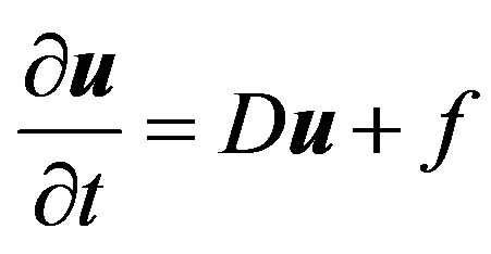
Consider a system of parabolic or hyperbolic partial differential equations
 (1)
(1)
where  is the solution vector, D is a linear or nonlinear matrix operator and
  is an explicitly given source (or forcing) term. Note that D may depend on both physical variables (t, x and u) and physical parameters (denoted p) and that f is assumed arbitrary but non-dependent on u. Initial u(t0,x;p) as well as (Dirichlet, Neumann or Robin) boundary u(t,xB;p) conditions are assumed known.
To avoid inverting a matrix solution vector, associated with the time derivative, Equation (1) is integrated in time;
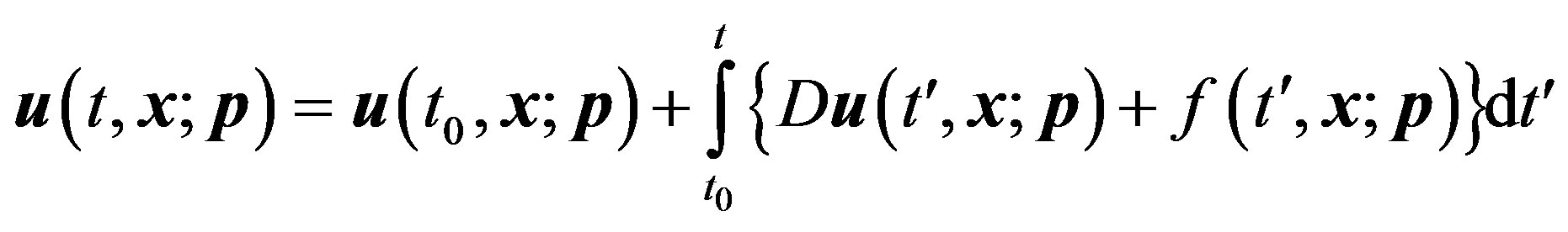 (2)
(2)
The solution vector  is approximated using first kind, multivariate Chebyshev polynomials series as both trial and weight functions. These polynomials, defined by Tn(x) = cos(ncos–1x), are orthogonal within the interval [–1,1] over a weight function (1 – x2)–1/2. Chebyshev polynomials may be defined appropriately to any given finite range [a,b] of x (shifted Chebyshev polynomials) by a linear transformation [2]. Confining us here to one spatial variable x and one parameter p, we thus have
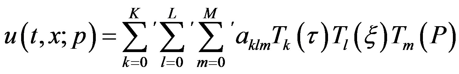 (3)
(3)
using the transformations
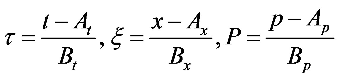 (4)
(4)
with ,
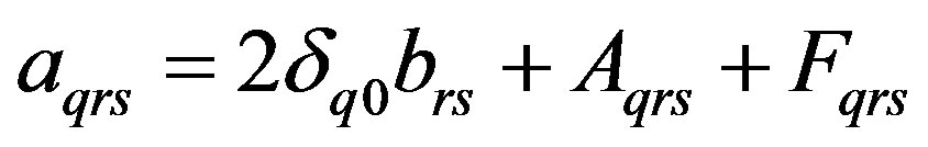
,  and where indices “0” and “1” denote lower and upper computational domain boundaries, respectively. Primes on summation signs in Equation (3) indicate that each occurrence of a zero coefficient index renders a multiplicative factor of 1/2. Just as for standard weighted residual methods (WRM), the unknown coefficients aklm are determined by requiring that the integral of the weighted residual over the computational domain should be zero. Performing the integration by parts, the result is [1]
 (5)
(5)
Here Aqrs and Fqrs correspond to Chebyshev expansions of the time integrals on the right hand side of Equation (2). Since Aqrs usually includes u itself, it usually is a polynomial function of the unknown coefficients aklm. For nonlinear equations, each element of relation (5) may thus be a complex function of the unknowns. The coefficients brs correspond to the Chebyshev expansion of the initial conditions. Equation (5), together with appropriate boundary conditions, is used to determine the GWRM coefficients aqrs that constitute the solution of the problem. Equation (5) can be linear or nonlinear depending upon the type of the problem. If linear, the coefficients can be found using traditional methods like Gauss elimination. For nonlinear problems, a semi implicit root solver (SIR) has been developed [5]. SIR has proven to be very robust for GWRM applications.
2.2. The GWRM and Finite Time Step Methods
In order to investigate the applicability of the GWRM, some test problems have been solved using the method [1]. The problems were also solved using the finite difference time step Lax-Wendroff and Crank-Nicolson methods. The former method is explicit and is subject to CFL (or similar) time step limiting conditions. The latter method allows for arbitrarily large time steps by using an implicit approach where the functional values are determined both at present and future time steps.
For studying accuracy, the nonlinear Burger equation
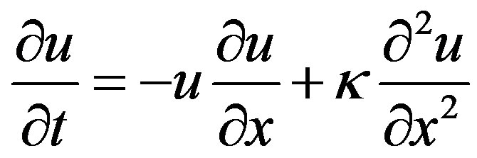 (6)
(6)
has been solved with initial condition 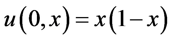 and boundary conditions
  for different values of
 . The results have been compared with the exact solution. Although the GWRM is primarily intended for computing long time behaviour of complex problems with several time scales, it can be used for accurate solution of stiff problems. For the case of Burger’s equation, the GWRM was shown to provide efficiency close to that of the Lax-Wendroff and Crank-Nicolson schemes for given accuracy. Improved GWRM efficiency is expected for problems with periodic boundary conditions. The GWRM has the additional advantage of providing approximate, analytic solutions.
For studying efficiency, a forced wave equation was solved:
 (7)
(7)
with ,
,  ,
,
 . Here A, n, α, β and v are free parameters, and f(t,x) = A(vβ2 – α2)sin(αt)sin(βx) is the forcing function. The exact solution is
 , (8)
, (8)
for β = mπ, with m an integer. This problem has the separate system and forcing function time scales
 and
and . Using the parameter values v = 1A = 10, α= π/15, β = 3π and n = 3, the ratio of these time scales becomes
 . Thus the forcing term in (7) has here introduced a time scale much longer than that of the “unperturbed” system.
It was found that the GWRM, as intended, is well suited for long time scale solution of this problem. For suitable mode parameters, it traces the slower dynamics using substantially less computational time than the Lax-Wendroff and Crank-Nicolson schemes. See Figure 1 for the case K = 6, L = 8, where single temporal and spatial subdomains are used. If results are sought for longer times, temporal subdomains are preferably used for the GRWM, in order to guarantee constant computational effort per problem time unit. For problems with wider separation of the time scales, the GWRM will be an increasingly advantageous method as compared to the Lax-Wendroff scheme since the latter must follow the faster time scale. It may also be noted that the GWRM
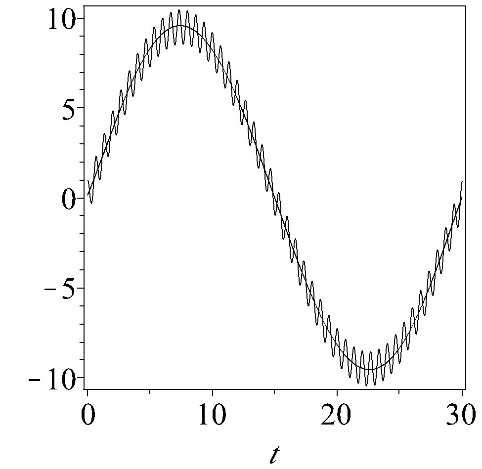
Figure 1. GWRM solution (smooth curve) of forced wave equation, as compared to exact solution (oscillating curve).
averages more accurately over the fast time scale oscillations than the finite difference methods. This is an interesting subject which deserves further attention.
The computations have been carried out using Maple. Although faster computational environments exist, exact comparisons of efficiency are not essential at this stage. The examples we have given show that the efficiency and accuracy of the GWRM is comparable to that of both explicit and implicit finite difference schemes in a given environment. Further optimisation of both GWRM and finite difference codes could increase efficiency, but our examples indicate that time-spectral methods for solution of initial-value pde’s are of interest for general use and for computations of problems in magnetohydrodynamic and fluid mechanics in particular.
3. Spatial Subdomains
The number of operations in GWRM computations can be significantly reduced by using subdomains for the spatial, temporal and physical variables [1]. It is the primary objective of this paper to qualify this claim. Thus we begin this section with some numerical considerations.
Iterative solution of the GWRM coefficient equation (5) will lead to approximately  = (K + 1)3(L + 1)3(M + 1)3 operations for each iteration owing to the cubic dependence on the number of unknowns for computations involving matrix inversion. Using LU decomposition methods rather than matrix inversion, the number of operations may be reduced to
  [6]. This may be an acceptable amount of work. For more complex calculations, however, high efficiency often requires the temporal and spatial domains to be separated into subdomains. This would in principle enable a linear rather than a cubic dependence of efficiency on, for example, the number of spatial modes applied to the entire domain, given that the number of subdomains is proportional to L. Now assume that the temporal and spatial domains are divided into Nt and Nx subdomains, respectively. The result is that only
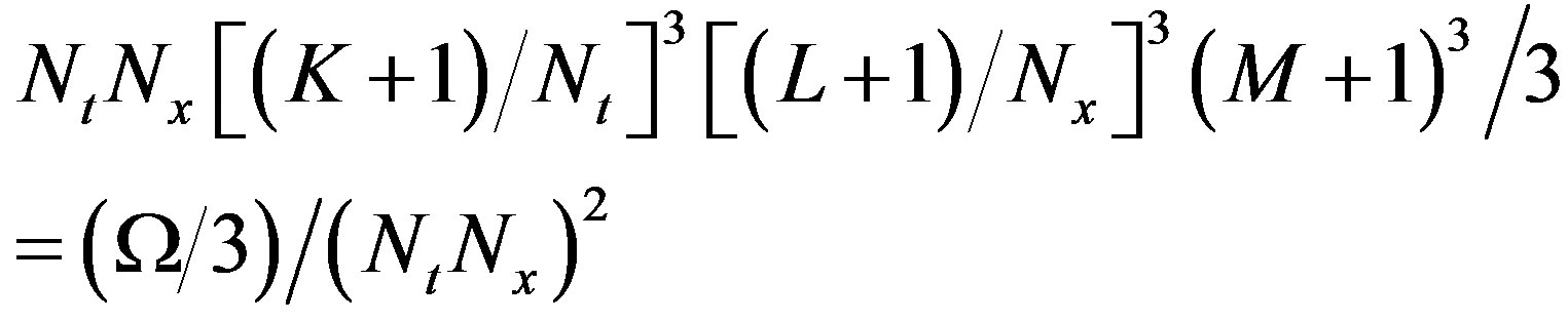
operations are then needed for a particular problem, assuming that the same total number of modes (degrees of freedom) are sufficient in both cases. As an example, for K = L = 11, M = 2 and Nt = Nx = 3 there would be a reduction from about 2.7 × 10⁷ to 3.3 × 10⁵ operations.
In this section, we will discuss and suggest schemes for introducing spatial subdomains. We begin by considering the question of how internal boundaries optimally should be constructed and how they depend on the spatial order of the differential equation. Next we turn to discuss how the subdomain conditions may be iterated as the solution is produced.
3.1. Internal Boundaries and Their Modelling
Whereas temporal subdomains are fairly easy to implement, spatial subdomains must be carefully handled. The reason is that, for spatial subdomains, the information that should be passed on between each subdomain is externally unknown and globally dependent on all other subdomain boundaries. For temporal subdomains the information at one boundary (the initial time) is completely known, thus numerically more stable behaviour may be expected.
A question arises. Given the spatial order  of the combined system of partial differential equations, what is the order of contact required between the internal spatial boundaries in order to avoid underdetermining the system? Clearly, continuity of the function itself and of its derivative are natural conditions. We may reformulate the problem by instead asking the question: given that the points of contact between the subdomains are given by continuity of the function and its spatial derivative only (second order contact), what requirements need be satisfied to avoid underdetermination of the system?
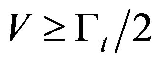
In the Appendix we show that the answer may be simply expressed as the criterion
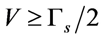 (9)
(9)
where V is the number of dependent variables that are used in the partial differential equation. Note that the number Ns of spatial domains has no influence. As an example, consider a fourth order equation ( = 4). If second order contact is used at internal boundaries, the equation has to be broken down into at least two second order equations to satisfy the requirement on information (9), that is V ≥ 2. This is, of course, easily facilitated.
Implementation of second order contact between the subdomains is not straightforward, however. Derivatives of Chebyshev expansions are spectrally represented as
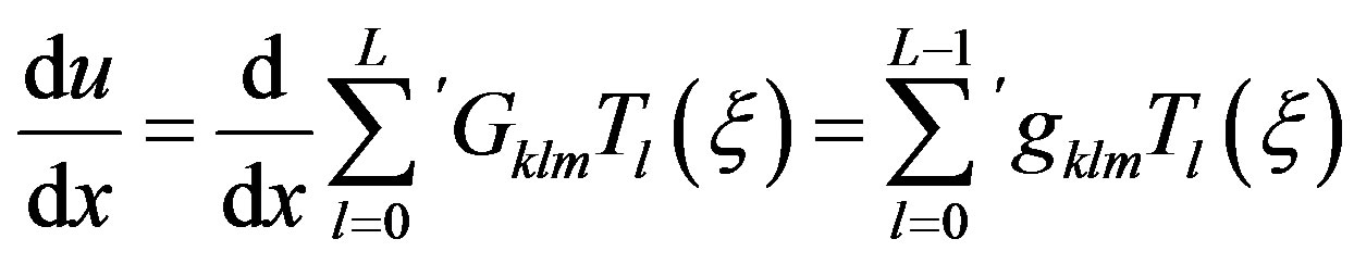 (10)
(10)
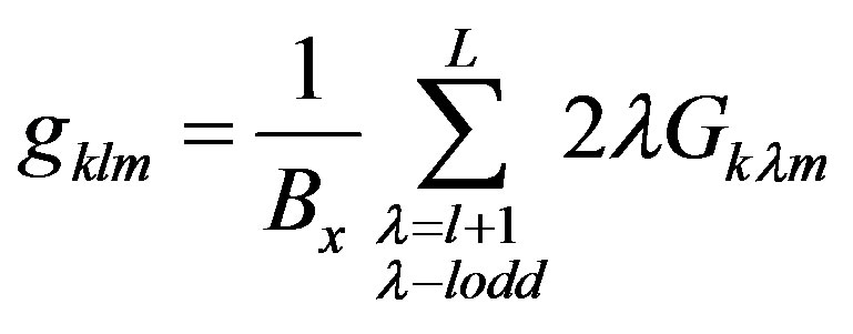
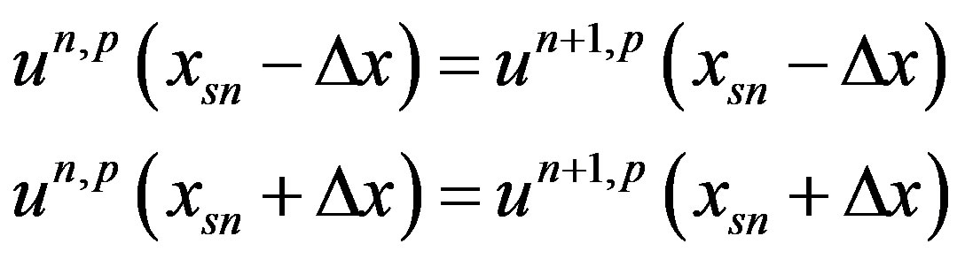
Even if the spectral coefficients Gklm associated with the function u converge, the convergence of the derivative is weaker because of the multiplying factors λ that add extra weight to higher order Gklm coefficients. In order to avoid consequential numerical instability, we have found that an overlapping (“handshaking”) procedure is preferable. The Chebyshev expansions of the dependent variables of each subdomain are allowed to extend a distance ∆x into the neighbouring domains. For simplicity we restrict us here to discuss a one-dimensional spatial domain. Assuming Ns spatial domains, external and internal boundary conditions relating to the dependent variable u are then implemented through
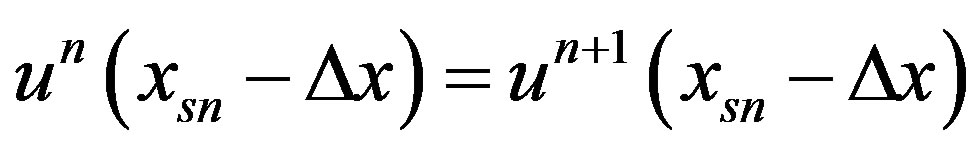
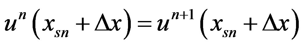
 (11)
(11)
for 1 ≤ n ≤ Ns – 1 with xsn denoting the position of the right-hand boundary of the nth subdomain un. The total number of external boundary conditions, that should be applied at the boundaries x0 and x1, is . The set {xsn} of internal boundaries need not be equidistantly spaced, and the size of ∆x may also be adapted to each subdomain, depending on, for example, the local stiffness of the problem. We will here constrain us to equidistantly spaced subdomain boundaries having the same values of ∆x, the size of which should be optimized.
We have studied different implementations of spatial subdomains of the form (11). These are now briefly described.
3.2. Method I—Dependent Subdomains
In this approach, the complete system of all coefficients 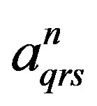 given by Equation (5) for all domains, including internal and external boundary conditions are solved selfconsistently at each iteration. For the internal boundaries it thus holds that, after each iteration p,
 (12)
(12)
This approach requires only a few iterations (typically 4 - 10 for nonlinear problems) for good accuracy and converges swiftly but on the expense of computational memory, as this involves matrix inversion of a large matrix, simultaneously representing all subdomains. A reason for employing several dependent subdomains in preference for a single spatial domain is that it may be economic to localize one or more subdomains in a region of strong gradients for an elsewhere smooth solution.
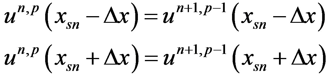
3.3. Method II—Independent, Consecutively Updated Subdomains
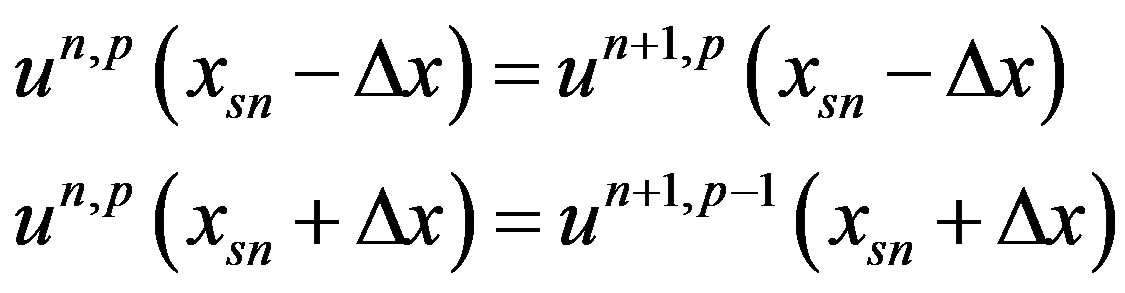
Here Equation (5) is iterated separately for each subdomain, with internal boundary conditions at point  obtained from the previous iteration, but with internal boundary conditions at point
  obtained from the neighbouring subdomain at the present iteration. Formally,
 (13)
(13)
This procedure decouples the matrices to be inverted at each iteration (one for each subdomain), and substantial computational speed is gained. A disadvantage is that a larger number of iterations is needed than for the case of dependent subdomains.
3.4. Method III—Independent, Late Update of Subdomains
This procedure differs from that of independent, consecutively updated subdomains only by that the internal boundaries are not assigned until all subdomains are computed at each iteration level:
 (14)
(14)
3.5. Retarding Update of Internal Boundary Conditions
Whereas explicit theoretical criteria for convergence may be formulated for the single domain problem, corresponding to solution of a fixed system of nonlinear equations, the situation is different for independent domains. The reason is that those coefficients of Equation (5) that correspond to the internal boundary conditions are non-constant throughout the iterations. If these were constant, convergence of each subdomain would, of course, be guaranteed once the convergence criteria were satisfied. In this case, however, no information is passed between the internal boundaries and a global solution is not attained.
On the other hand, if boundary information changes too rapidly during the iterations of Equation (5), the iteration scheme may not lead towards a solution and convergence is endangered. Intuitively, a possible remedy would be to “retard” the information exchange at the internal boundaries by only allowing for a certain rate of change. The boundary data that comes into iteration p are thus replaced by a weighted combination of boundary value data from both iterations p – 1 and p – 2. This procedure is likely to be successful, since in the limit that all boundary data are obtained from the previous iteration (that is, the boundary conditions are unaltered throughout the iterations) well known convergence criteria exist. The internal boundary equations (11) are consequently replaced with the following set of relations:
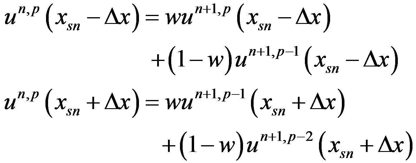 (15)
(15)
The parameter w is used to control the weight of “new” boundary information in relation to “old” boundary information. For w = 1, the scheme degenerates to the case of independent, consecutively updated subdomains, and for w = 0 the conditions at the internal boundaries remain fixed. In the following, we will refer to this procedure as the “w method”.
4. Temporal Subdomains
As described in Section 3, temporal subdomains can enhance computational efficiency of the GWRM. Similarly as for spatial subdomains, the major role is played by the reduction in operations when inverting the matrix for each domain, required for solution of the coefficient Equation (5). For instance, a temporal domain using K modes could simply be split up into Nt subdomains with  modes in each. Stiff differential equations, however, may of course require somewhat more than
 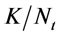 modes per subdomain for adequate accuracy, reducing the gain in efficiency. As was also shown in Section 3, optimal efficiency is likely obtained when spatial and temporal subdomains are employed jointly.
There are essentially two different paths to implement temporal subdomains, using single or multiple order contact at the temporal boundary. For single order contact, the result from the previous temporal subdomain at time t = t1 is simply used as initial value at time t = t0 for the subsequent time domain. This is not always allowed: similarly as for spatial subdomains, the number of external conditions to be imposed on each variable depends on the order of the system. Single order contact requires that there are at least as many variables as the temporal order of the combined differential equations. Since the GWRM system of equations are always cast in the form of Equation (1), this is always guaranteed for GWRM problems. Application to a large system of differential equations will be presented in the next section.
For second order contact in the temporal domain, the condition
 (16)
(16)
must be satisfied. This result is found in a similar manner as the condition (9) for spatial subdomains. Here  is the order of the time derivative for the system. Second, or higher, order contact is not necessary for GWRM applications, but may improve convergence, in particular in presence of shocks. This is a matter for future study.
Adaptive, temporal subdomains can enhance accuracy and efficiency. To introduce the adaptive temporal subdomain method for nonlinear problems, a stiff ordinary differential equations is here studied. The following equation models the propagation of the flame when lighting a match:
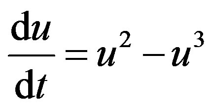 (17)
(17)
It is assumed that u(0) = δ and that . This is a stiff differential equation for small values of the parameter δ because of the presence of a ramp at
 .
.
We have solved this problem by using routines for transforming nonlinearities to Chebyshev spectral space and by formulating an equation of the form (5); see Ref. [1]. A strongly ramped solution with δ = 0.0001 is computed. We have imposed an accuracy of ε = 1.0 × 10⁻⁴ by comparing the GWRM solution with the exact solution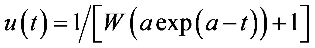 , where
 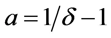 and W is the Lambert W function. Both the computed and exact solutions are shown in Figure 2. At this accuracy, they are indistinguishable from each other.
Also, the smallness of δ makes the ramp very distinct and numerically difficult to resolve. Consequently, explicit finite difference methods need extremely small time steps to solve the problem. An optimised Matlab solution uses implicit methods that reduces the computational effort to about 100 time steps, taking a few seconds on a tabletop computer.
The GWRM solution uses 69 time domains and takes just about the same amount of computational time. The temporal domain length has been automatically adapted as follows. Since it holds that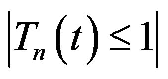 , a useful accuracy criterion is
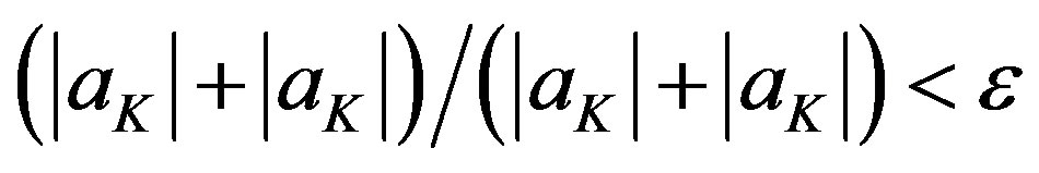 , where an is the nth coefficient in the Chebyshev spectral expansion of u.
In performing the adaptive computation, a default of 10 time subdomains is assumed and K = 6 is used. If the accuracy criterion is satisfied, the subdomain length is doubled at the next domain, and if not it is halved. In the latter case, the calculation is repeated for the same subdomain until the accuracy criterion is satisfied. This goes on as the calculation proceeds in time until near the endpoint, where the subdomain length is adjusted to land exactly on the predefined upper time limit. Due to the stiffness of the problem, the subdomains are concentrated near t = 1.0 × 10⁴ where the subdomain length may be as small as about 2 time units. The automatic extension of the subdomain length in smoother regions saves considerable computational time; at the end of the calculation the subdomain length is more than thousand time units.
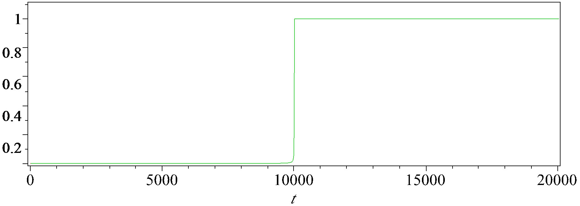
Figure 2. GWRM and exact solutions of Equation (17) for δ = 0.0001.
5. Results
Accuracy and computational efficiency of two example problems will now be studied, employing the above discussed three GWRM spatial subdomain methods. Also, the effect on convergence by use of the w method (Section 3.5) will be studied.
5.1. Burger Equation—Spatial Subdomains
The Burger Equation (6) is a fundamental hyperbolicparabolic partial differential equation from fluid mechanics, containing both convection and diffusion terms. Thus two separate time scales govern the time evolution of an initial state.
We showed in Section 2 that GWRM accuracy is comparable to that of explicit and implicit schemes, for a similar number of floating operations. For high accuracy, that is at high mode numbers, it is of interest to determine whether spatial subdomains may reduce the memory requirements and the number of operations. Employing the methods described earlier we compare the results with the analytical solution given in Ref. [1], using 50 terms of the expansion.
The results for Method I are displayed in Table 1 for a suitable selection of parameters. Initial and boundary conditions are those stated below Equation (6) and we have chosen  = 0.01. By “Iter” is meant the number of iterations required, “Time” denotes the normalized time required to solve the GWRM system of coefficient equations (5) including boundary conditions, “Memory” denotes normalized memory requirements and “Max error” is the maximum absolute error as compared to the exact solution. The maximum mode number L for subdomains is obtained from the relation
 . The root solver SIR is set so that it solves system (5) using Newton’s method, with start data given by the initial condition. It is seen that convergence is rapid for all cases, even when 5 subdomains are employed. The primary information from Table 1 is that although computational time and memory requirements decrease when employing the relation
  for the spatial subdomain modes, accuracy is partially lost. Due to the shock-like structure of the solution near r = 1, many modes are needed for high resolution. We will return to this issue.
Next, the same problem is solved using Method II. The results are displayed in Table 2. Clearly, less memory is used than in Method I but more iterations are required, thus enhancing computational time. The convergence of all Ns = 5 cases was too slow to reach a SIR solver accuracy of 1.0 × 10⁻⁵ within 100 iterations. For the convergent cases, the absolute error is essentially the same as for Method I.
It becomes of interest to determine whether the w
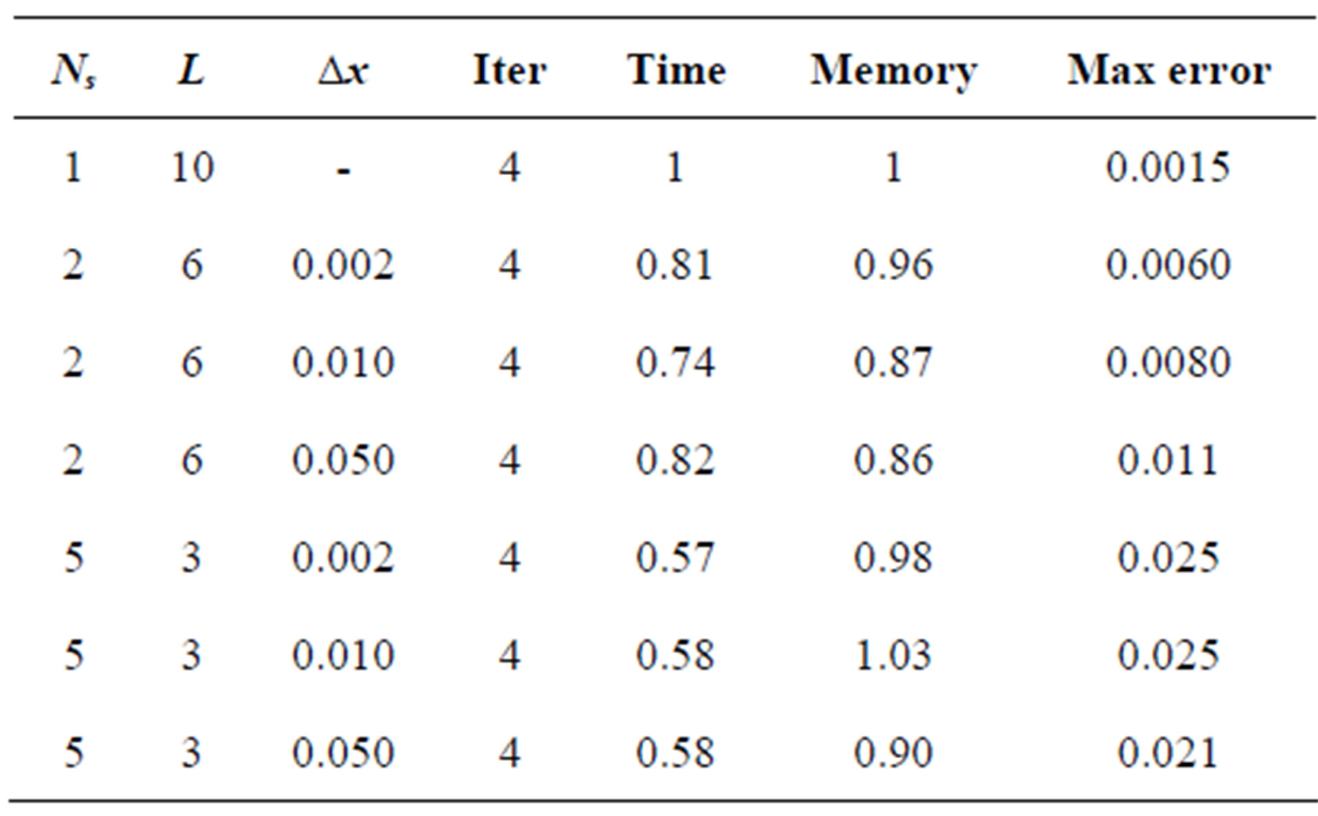
Table 1. Method I solution of Burger’s equation.
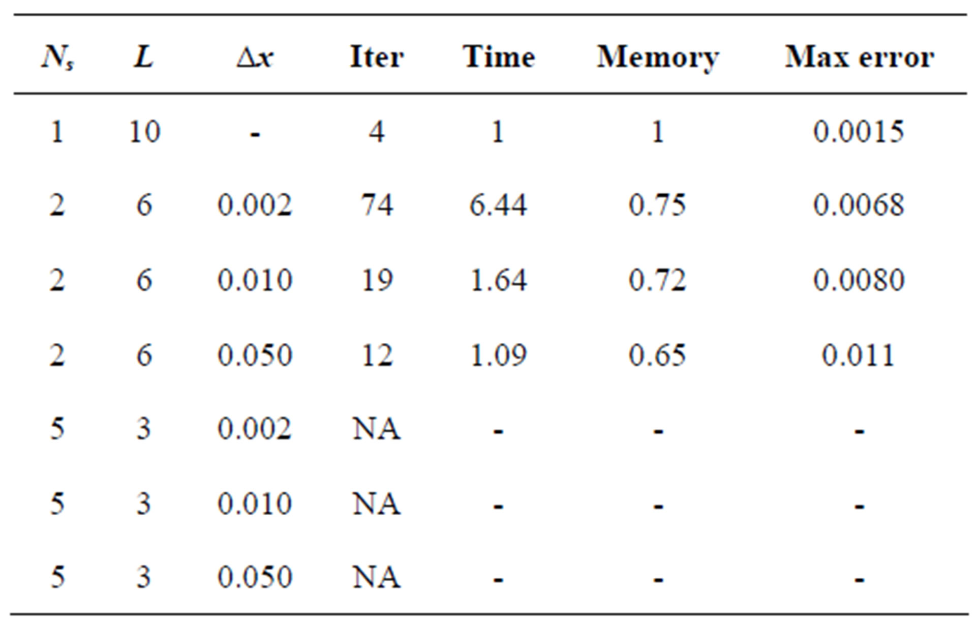
Table 2. Method II solution of Burger’s equation.
method described in Section 3.5, using the weighting parameter w, can improve convergence of Method II. Results are shown in Table 3.
The values of w given indicate the values that result in the least number of iterations of Equation (5). We find that convergence can be improved using the w method, in particular for the case with several spatial subdomains. The w method is most effective for large .
.
Finally, we return to the question how many spatial modes are required in each of several subdomains to obtain the same accuracy as that of the single domain for the Burger equation. Results are shown in Table 4, using Method II. It is seen that Method II offers a path to comparable accuracy using less memory, at the expense of computational time.
For all cases considered, Method III converges slower than Method II; thus we do not report on any details of these calculations. The result is not surprising, since Method II can be regarded as a hybrid method in relation to Methods I and III in the sense that one subdomain boundary is instantaneously updated as the coefficients of each subdomain are iterated using Equation (5).
Let us summarise the results from application of spatial subdomains. Regarding convergence, we conclude that Method I converges fast for all cases considered. Method II needs more iterations and does not converge at
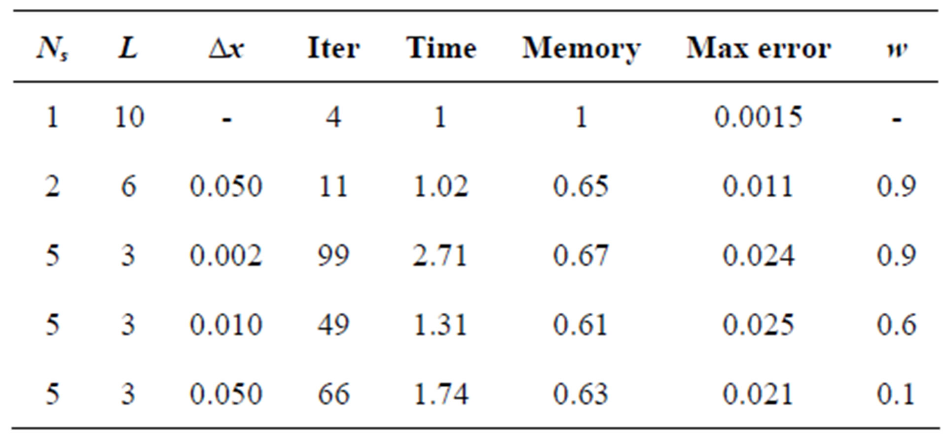
Table 3. Method II solution of Burger’s equation.
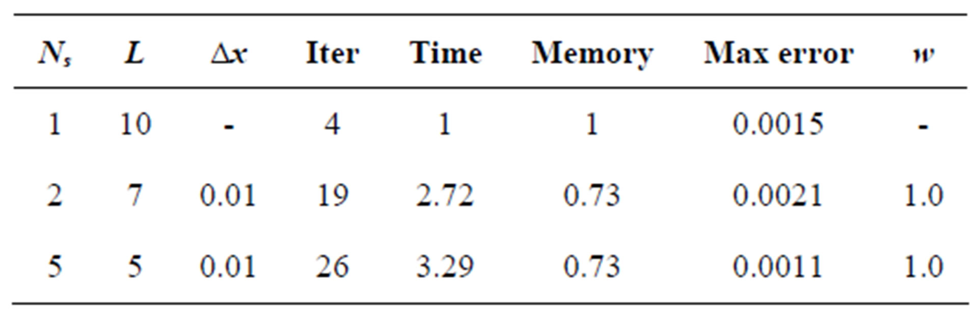
Table 4. Method II solution of Burger’s equation, higher accuracy.
all for cases featuring many subdomains. Employing the w parameter method, however, Method II convergence is obtained for nearly all cases. Method III generally features poorer convergence properties than Method II.
Accuracy is high for the single subdomain case, since the Burger equation features a shock near r = 1, where high spectral orders are needed for good resolution. Method II reaches the same accuracy both for the case of 2 and 5 subdomains when the order of the Chebyshev spectral expansion is 7 and 5, respectively. This shows that for shock-like problems, the order of the spectral expansions needed in each domain is higher than , that is, the total number of degrees of freedom must be increased. For the same values of Ns and L, all methods provide the same accuracy.
Computational memory requirements are the highest for Method I, since it involves a global solution where all Chebyshev coefficients are simultaneously interrelated at each iteration. Memory reductions by up to 40% were demonstrated for Method II. The reduced memory requirement is coupled to the size of the matrix equations corresponding to Equation (5), and for both Methods II and III a substantial increase in efficiency in the sense that the iteration computational time is reduced to a fraction of that of the single domain case. The number of iterations required are higher for Methods II and III, however, and the total computational time becomes comparable to, or higher than, that of Method I.
In conclusion, using a simple but demanding test problem we have shown that spatial subdomain methods, in combination with the w method, has a potential to alleviate memory requirements for the GWRM while preserving accuracy and, in most cases, convergence. Efficiency is, however, reduced for these cases.
5.2. Magnetohydrodynamic Equations—Spatial and Temporal Subdomains
We next turn to an advanced application of GWRM subdomain methods. The problem at hand is a plasma stability problem formulated as a system of coupled magnetohydrodynamic (MHD) equations. The following set of equations govern the resistive MHD model:
 (18)
(18)
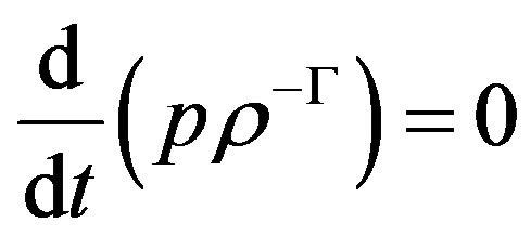
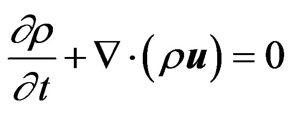
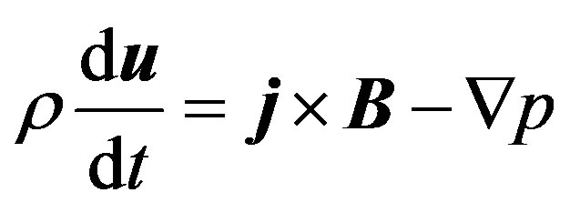
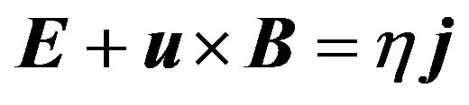
These macroscopic (fluid) plasma equations are the continuity and momentum equations, Ohm’s law (including resistivity) and the (adiabatic) energy equation followed by Faraday’s and (the displacement current free) Ampere’s law, respectively. Regarding notation, E and B denote the plasma electric and magnetic fields respectively, u is the fluid velocity, j is the current density, p is the kinetic pressure, ρ is the mass density, η is the resistivity, Γ = 5/3 is the ratio of specific heats and μ0 is the vacuum permeability. The MHD stability problem consists of a system of 14 nonlinear, coupled partial differential equations. Boundary conditions corresponding to a perfectly conducting wall are provided from the requirements that the radial components of the magnetic field and fluid velocity should vanish, and from the fact that the parallel components of the electric field at the wall should vanish. For further details, see Ref. [7].
A standard way of investigating plasma stability is by linearization of the above equations followed by Fourier decomposition in the azimuthal and axial directions (circular cylindrical geometry is assumed here). All dependent quantities Q are considered as the sum of an equilibrium term Q0 and a small perturbation q, thus Q = Q0 + q. Perturbations are assumed to be proportional to exp[i(mθ + kz)] where k and m are the axial and azimuthal mode numbers respectively. For a given perturbation, stability is completely determined by the equilibrium. An equilibrium is unstable if it features a time dependence exp(γt), where γ is a positive number, and stable (wavelike solution) if γ is imaginary.
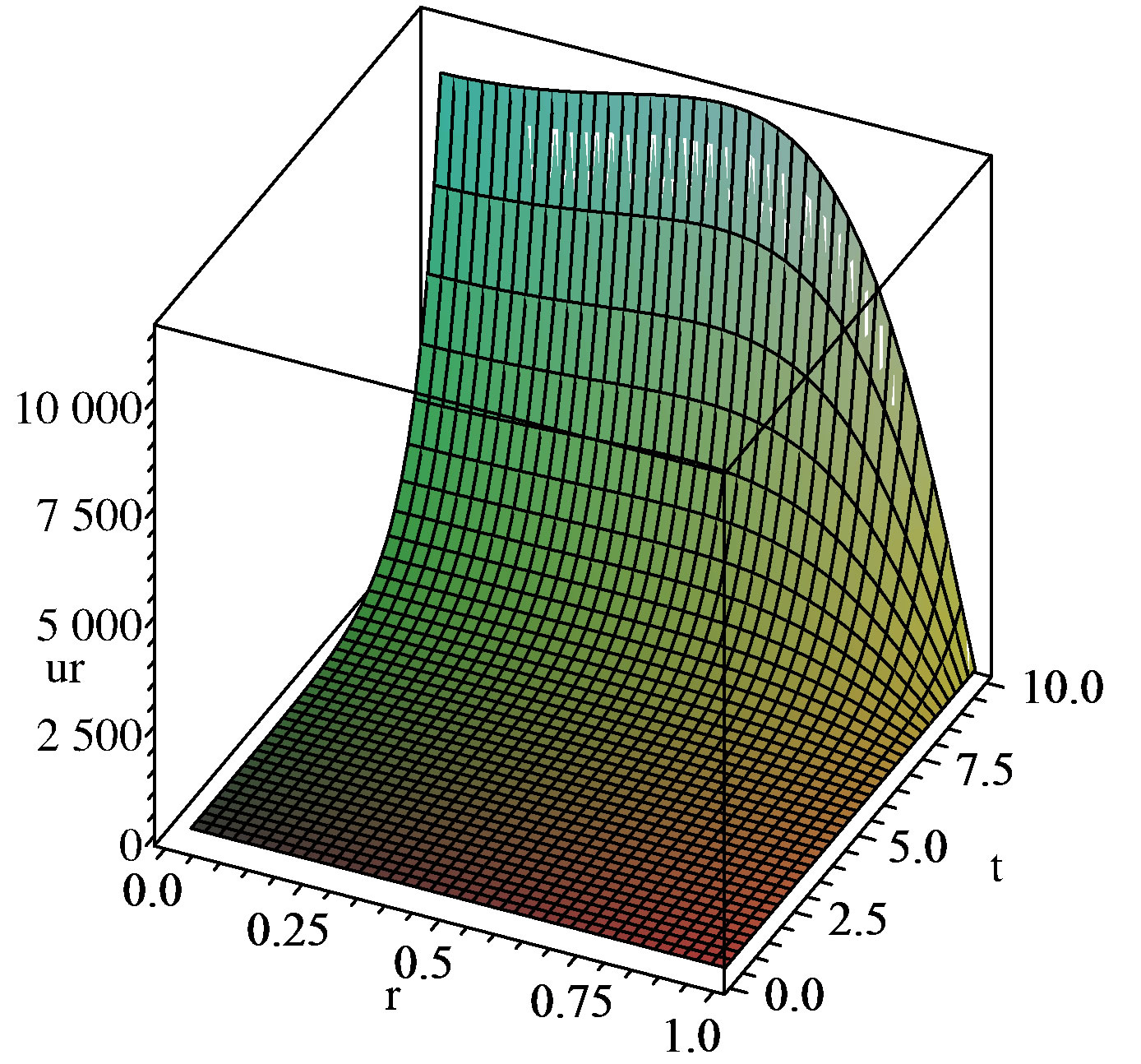
The equations (18), together with initial and boundary conditions, have been solved with the GWRM for a number of different equilibria. We here study the stability of the z-pinch equilibrium B0θ = r, B0z = 0, p0 = 1 – r2, where r denotes the radial coordinate. Also, it is assumed that ρ = constant and that η = 0. The effect of an initial perturbation (m,k) = (1,10) is followed for a sufficiently long time that a dependence of the form exp(γt) has time to develop. The solution to this problem is known from computations using other methods. We have applied both Methods I and II to this problem. In Figure 3(a) is displayed the evolution in time and space of the radial, perturbed fluid velocity, using Method I with 5 temporal subdomains (Nt = 5) and a single spatial domain, using orders K = 5 and L = 10 and a time domain reaching to 10 normalized (Alfvén time) units. The equilibrium was unstable for this perturbation. Obtained growth rate is γ = 1.03, to be compared with the correct result γ = 1.04.
In Figure 3(b) the same method is used for 5 temporal domains, but now for 3 spatial domains using  = 0.05 and with orders K = 4 and L = 3. The obtained growth rate was γ = 1.06. In comparison with the single subdomain case, 81% of the computational time was
 (a)
(a)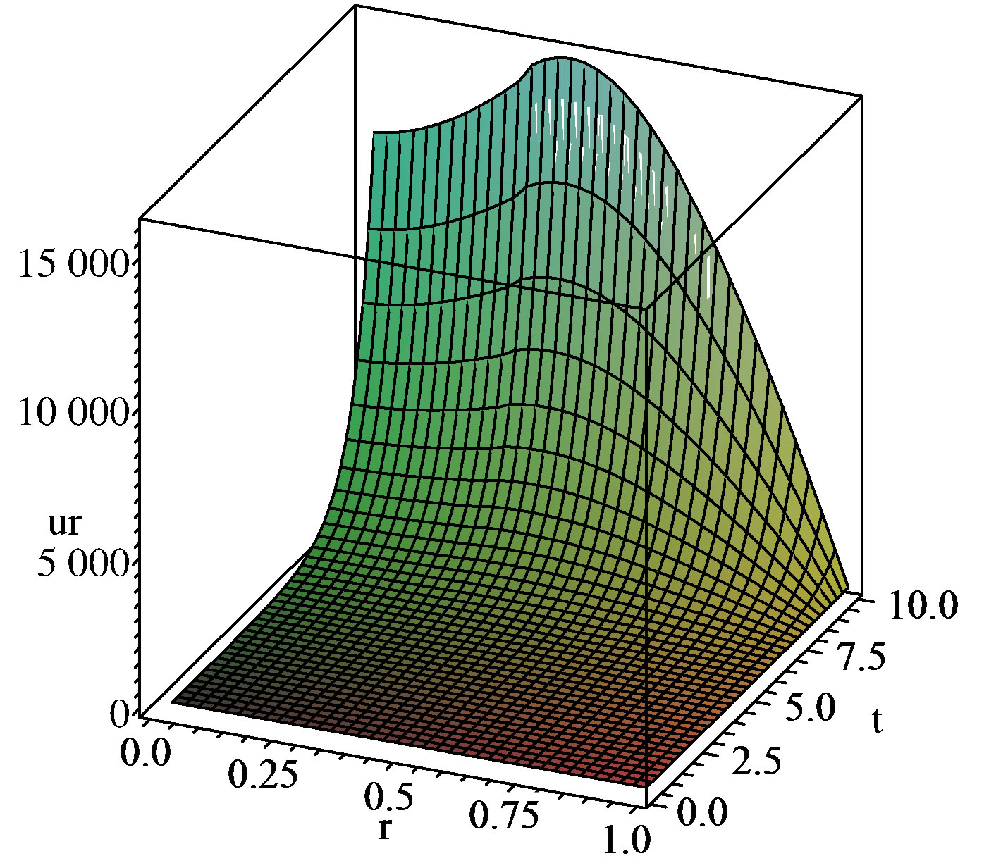 (b)
(b)
Figure 3. (a) GWRM single spatial domain solution of an MHD stability problem formulated using Equations (18), showing radial velocity ur . Method I was used with Ns = 1, Nt = 5, K = 5, L = 10; (b) GWRM solution as in Figure 3(a), but here Ns = 3, ∆x = 0.05, Nt = 5, K = 4, L = 3.
needed, with a memory requirement of 82%.
It should be noted that relatively high values of K would be required for this case for sufficient accuracy if a single temporal domain were used. This is due to the exponential dependence of the solution, which requires high order spectral resolution. Using orders K = 5 and L = 10, the value γ = 0.73 was found, and at sufficiently high values of K, the internal Maple memory (on a table-top computer, order 250 Mb) was insufficient.
Application of Method II was unsuccessful; convergence could only be obtained for impractical subdomain time intervals (<0.1 time units). This being in spite of application of the w method, and of various techniques to expedite convergence.
Although this is a linear problem in the unknown variables, iterations are needed to satisfy the internal boundary conditions, since the subdomains are partially decoupled. Thus the SIR solver was fruitlessly tried with various values of its convergence parameters.
Likewise, Method III was unsuccessful in handling this complex problem. The reason is found in that, whereas Method I retains the acausality of the GWRM, Methods II and III introduces independent spatial regions that become coupled to the length of the time interval through a CFL-like criterion. Thus, time domains must be kept small for convergence.
6. Discussion
The GWRM convergence of problems with a single spatial domain is often adequate, but memory requirements may be large when many spatial modes are employed for obtaining high accuracy. This is mainly due to that a matrix equation for all GWRM coefficients need be solved at each iteration by a root solver, a procedure that scales as L3 operations.
By employing a set of spatial subdomains, memory requirements may be reduced. Spatial subdomains are here implemented in three different ways. In Method I, the internal boundary conditions of all subdomains are simultaneously solved for at each iteration; see Equation (12). This still requires the use of a single, global matrix equation for the GWRM coefficients. In Method II, the subdomains are decoupled so that the connecting internal boundary conditions are updated consecutively at each iteration; see Equation (13). Finally, in Method III the internal boundary conditions are updated jointly at the end of each iteration; see Equation (14). It is in the two latter cases that the main potential for reduction of memory requirements exists, and thus of efficiency in solving the GWRM matrix equation. If  spectral modes are employed at each subdomain,
  operations would be performed for coefficient matrix solution at each iteration. This represents a gain in efficiency by a factor
 . We show that, in order to retain accuracy, more modes are needed in each subdomain, so the gain in efficiency is somewhat reduced for the same accuracy.
Usually Methods II and III require more iterations than Method I. The cause for this is that the information of the internal boundary conditions is changing rapidly. By introduction of a weighting parameter w, we have shown that by controlling the rate at which information enters the internal boundary conditions, otherwise numerically unstable cases may be stabilized. For nearly all cases studied in this work, Method II has turned out to be preferable to Method III.
All three methods have been employed to solve the example magnetohydrodynamic stability problem. This is an advanced problem, since it involves the simultaneous solution of 14 coupled partial differential equations, with a rapidly (exponentially) growing solution. Method I was successfully applied, both for single and multiple spatial subdomains and using multiple temporal domains. Whereas Methods II and III were applicable to the Burger example, they were however ineffective for this case in the sense that unrealistically small time domains were essential for convergence. We speculate that this behaviour is related to the causal behaviour that is imposed by partially decoupling the subdomains (except for boundary points) from each other. Spatial decoupling implies a CFL-like condition to be satisfied. For Ns = 3, it would thus seem that the time interval  may not exceed the ratio of characteristic length (1/3 in normalized units) to characteristic speed (1 in normalized units), thus being approximately equal to 1/3 time units. The w method was shown to add increased stability, but convergence remained unrealistically slow for all values of w. Turning to the Burger case, the explicit finite difference stability criterion is approximately [1]
 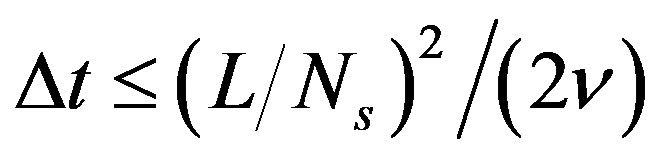 = 2 for Ns = 5. This may explain the need for the w method here.
We have employed the SIR root solver [5], with parameters set to make it identical to Newton’s method, for inversion of the GWRM matrices of this work. Starting points for the iterations was chosen to be the initial conditions of the problems. It should be mentioned that further optimization of convergence may be aquired by adjusting the parameters of SIR.
Temporal GWRM subdomains were studied for first order contact applications since the GWRM equations are formulated as a set of first order partial differential equations, and are easy to implement. Nonetheless, second or higher order contact in time should be considered in future work to improve convergence for advanced problems.
7. Conclusions
Implementations of spatial and temporal subdomains for the generalized weighted spectral method (GWRM [1]) have been demonstrated. In this method, also the time domain is given a spectral representation in terms of Chebyshev polynomials.
Two example applications have been used; the nonlinear Burger equation and a system of 14 coupled magnetohydrodynamic equations. Three different methods employing spatial subdomains were introduced. Whereas the first involved simultaneous solution of all, global Chebyshev coefficients, the other two have the potential of being computationally less demanding because their corresponding Chebyshev coefficient matrix equations are iterated separately at each iteration step.
It was found that temporal subdomains are essential for efficiency for both high accuracy and extended time computations. Solving a stiff ordinary differential equation it was shown that an adaptive GWRM time domain formulation compared well with commercial software both regarding efficiency and accuracy.
8. Acknowledgements
We gratefully acknowledge helpful discussions with Dr. Thomas Johnson.
REFERENCES
- J. Scheffel, “A Spectral Method in Time for Initial-Value Problems,” American Journal of Computational Mathematics, 2012.
- J. C. Mason and D. C. Handscomb, “Chebyshev Polynomials,” Chapman and Hall/CRC, New York, 2003.
- R. Peyret, “Spectral Methods for Incompressible Viscous Flow,” Springer-Verlag, Berlin, 2002.
- C. Canuto, M. Y. Hussaini, A. Quarteroni and T. A. Zang, “Spectral Methods, Evolution to Complex Geometries and Applications to Fluid Dynamics,” Springer-Verlag, Berlin, 2007.
- J. Scheffel and C. Håkansson, “Solution of Systems of Non-linear Equations—a Semi-implicit Approach,” Applied Numerical Mathematics, Vol. 59, No. 10, 2009, pp. 2430-2443. doi:10.1016/j.apnum.2009.05.002
- W. H. Press, S. A. Teukolsky, W. T. Vetterling and B. P. Flannery, “Numerical Recipes,” Cambridge University Press, Cambridge, 1992.
- J. Wesson, “Tokamaks,” 2nd edition, Clarendon press, Oxford, 1997.
Appendix
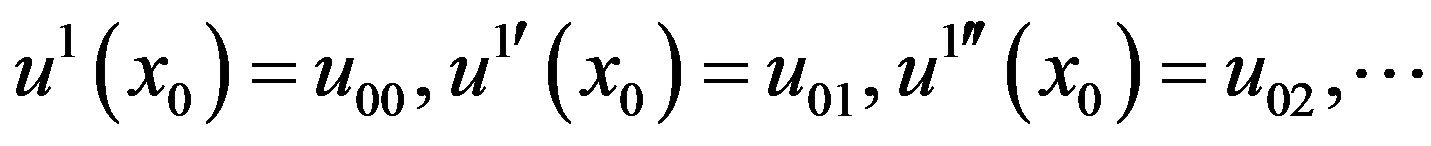
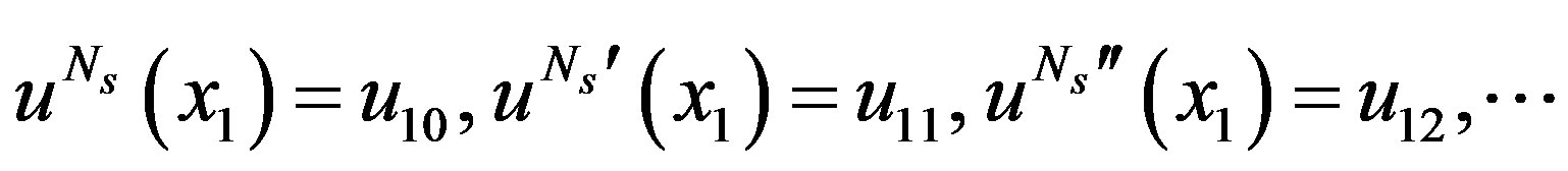
In this Appendix, we derive a criterion for the minimum number H of contact points required at the internal boundaries in order to determine, and not underdetermine, an approximate solution that uses the full information from both the system of differential equations and from the external boundary conditions. H will be a function of the spatial order of the system of differential equations , the number of spatial subdomains Ns and the number of variables V. The analysis is restricted to a single spatial dimension but can easily be generalized to higher dimensions. The criterion can also be applied to temporal domains. We assume that the approximate solution can be expressed as a truncated expansion in some basis, for example Chebyshev polynomials.
The total number of unknown coefficients of the system that must be given information is , since the solution for each variable in each subdomain needs information in the form of
  relations to be completely determined. The differential equations will provide for information to solve for all but
  of these in each subdomain. Thus, in total, the differential equations will provide
  equations. This gives the total number of internal boundary conditions that are needed;
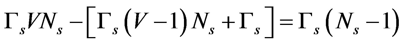
where contributions from  externally given boundary conditions have been accounted for.
The  external boundary conditions may be applied on any variable, at any external boundary and for any order less than
 . The two outermost spatial subdomains related to each variable also have contact with the inner subdomains. These points add upp to HV in total. The desired criterion can now be derived from the requirement that the average number of internal contact points
 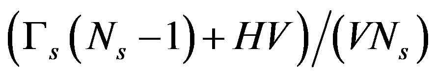 should be less or equal than H. Solving this equation, there results the criterion
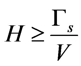 (A1)
(A1)
The criterion is independent of , as it should be. For “double handshaking”, that is for H = 2, we see that condition (A1) is easily satisfied for the magnetohydrodynamics problem of Section 5.2, for which
  = 6 and V = 7. Additional contact points near each internal boundary may of course be added for computational reasons.