American Journal of Computational Mathematics
Vol.2 No.1(2012), Article ID:17952,9 pages DOI:10.4236/ajcm.2012.21002
A Parameter Estimation Model of G-CSF: Mathematical Model of Cyclical Neutropenia
1Department of Mathematics, Sri Ramanujar Engineering College, Chennai, India
2Department of Mathematics, B.S.Abdur Rahman University, Chennai, India
Email: *balamurali.maths@gmail.com
Received November 20, 2011; revised December 20, 2011; accepted December 30, 2011
Keywords: FFT Modeling; Cyclical Neutropenia; Neutrophil; G-CSF
ABSTRACT
We investigate the FFT (Fast Fourier Transform) model and G-CSF (granulocyte colony-stimulating factor) treatment of CN (Cyclical Neutropenia). We collect grey collies and normal dog’s data from CN and analyze the G-CSF treatment. The model develops the dynamics of circulating blood cells before and after the G-CSF treatment. This is quite natural and useful for the collection of laboratory data for investigation. The proposed interventions are practical. This reduces the quantity of G-CSF required for potential maintenance. This model gives us good result in treatment. The changes would be practical and reduce the risk side as well as the cost of treatment in G-CSF.
1. Introduction
All blood cells are derived from hematopoietic stem cells. These stem cells are called “undifferentiated cells”. They have high proliferative potential in nature. This multipotent stem cells which often regulates cytokines, erythropoietin, erythrocyte, thrombopoietin, platelets as well as granulocyte colony stimulating factor and regulates leukocyte numbers [1,2].
The mathematical form of “hematopoiesis” is present in the stem cells and it is examined in simple analysis here. Several hematological diseases which display dynamic and potential nature, which is characterized by “oscillations” and one or more circulating cell lines are analyzed in this investigation. This analysis reveals cyclical neutropenia, periodic chronic myelogenous leukemia, cyclical thrombocytopenin and periodic hemolytic anemia [3].
In this chapter, we examine cyclical neutropenia which is rarely leads to hematological disorder characterized by “oscillations” in the circulating neutrophil count. Sometimes the oscillation level may fall. The period of oscillation time may be of 19 to 21days in humans, even though it has been observed to 40 days. These “oscillations” are generally accompanied by platelets, lymphocytes and retriculocytes. Cyclical neutropenia also occurs in grey collies when the periods on the order may be of 11 to 16 days. This is called “animal model”. It has provided extensive experimental data too [4]. It enriched our understanding of cyclical neutropenia.
The cyclical neutropenia have been mostly identified in the “gene”. This dynamic origin of gene is partially understood by us time to time. Many of the mathematical models have been formulated by this method. The analysis of cyclical neutropenia lies in destabilization of the combined HSC and neutrophil control system [5,6]. This analysis presents the CN oscillations in general. The CN oscillations also present the platelets and reticulocytes. The CN in humans are often treated using granulocyte which is known as “apoptosis”.
The treatment protocols typically call for daily subcutaneous injection of G-CSF at 3 to 5 μg per kg of body weight. This cost over US $45,000 per year for a 70 kg adult. A few alternative strategies in humans have been reported and various administration schemes have been used. In the two compartment models, HSC compartment was used and to hide the dynamic behaviour of the hematopoietic system under G-CSF treatment, the neutrophil count could be stabilized or to show large amplitude oscillations. This model G-CSF treatment schemes are effective while using less G-CSF. This model includes either erythrocyte or platelet dynamics even though clinical data indicates oscillations or neutropenia patients. This model would be consistent with observed platelet and gives reticulocyte data. After same time the stimulations are not taken into account. In this chapter [7-10], we present a new model which effects G-CSF treatment for cyclical neutropenia. Hence we enhance this model of the hematopoietic system by comparing it with two compartment modes of G-CSF kinetics. The details of the mathematical models are presented in detail [11-13].
2. Dynamic Hematological Diseases
Dynamic hematological diseases are characterized by oscillatory behaviours in one or more cell lines. They have been intensively modelled due to their interesting dynamic nature. In this chapter, we reinvestigate the basic characteristics of four periodic hematological disorders (periodic auto-immune hemolytic anemia, cyclical thrombocytopenia, cyclical neutropenia and periodic chronic myelogenous leukemia) and examine the role that mathematical modelling and numerical simulations played in our understanding of the diseases and regulations of hematopoiesis [14,15].
2.1. Mathematical Models of Hematopoiesis
Mathematical models have been used for modeling biological processes for decades. With the advances in technology and the increasing amount of available data, mathematical models and simulation techniques provide ways of better understanding the underlying mechanisms of biological processes. In hematological modeling, several mathematical tools and computational methods are used: differential equations (partial, ordinary or delay), stochastic processes, Boolean networks, Bayesian theory, multivariate statistics, decision trees, etc. The choice of the mathematical tools often depends on the desired level of description of the model. For instance, one could model processes at small scale (e.g. at the molecular or the cellular levels), or on a larger scale (model the whole system). Mathematical models of in vivo hematopoietic regulatory systems using a stochastic formulation have not been extensively developed, primarily because of the lack of corresponding data for stem cells and their progeny. Since they are widely used, we focus in this chapter on models that use differential equations: ordinary differential equations (ODE), partial differential equations (PDE), or delay differential equations (DDE) [13,16].
In this section, we first discuss the different types of delay differential equations and show how some DDE systems could be reduced to an ODE system using the linear chain trick. Second, we present a typical setting for a model, based on biological aspects of hematopoiesis and show that this could be modeled by an age-structured model (PDE). We then show that this PDE model can be reduced to a DDE model.
2.2. DDE Models
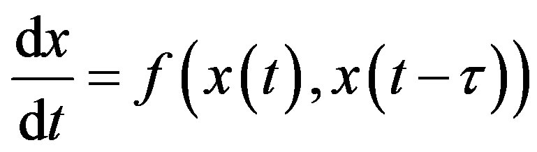
Delay-differential equations (DDEs) are a large and important class of dynamical systems [1,12,17]. They often arise in biological systems where time events naturally occur. In particular, in hematology several processes are controlled through feedback loops and these feedbacks are generally operative only after a certain time, thus introducing a delay in the system feedback. The general form of a DDE for  is
is
 (1)
(1)
where x𝜏 is the delayed variable  and f is a functional operator in R × Rn × C1. There are different kinds of delay differential equations: with discrete fixed delays, with distributed delays and with state-dependent delays. In this section, we briefly discuss these different types of DDEs and give some examples of how they have arisen in modeling hematological problems.
2.2.1. DDE with Constant Delays
Delay differential equations with constant delays take the form
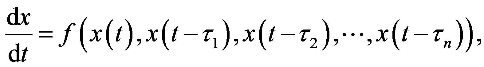
where the quantities 𝜏i, i = 1, 2, n are positive constants. For simplicity, consider the DDE with a single constant delay:
 (2)
(2)
To obtain a solution of Equation (13) for t > 0, one needs to specify a history function on [−𝜏, 0]. Indeed, recall that for an ordinary differential equation (ODE) system with n variables, one would only need to specify the initial values x(0) for each of the n state variables. In order to solve a DDE, one needs to specify not only the value at t = 0, but also all the past values of x(t) over the interval [−𝜏, 0]. Since one needs on specify an “infinite” number of values, DDEs are often viewed as infinitedimensional systems. Constant delay differential equations are often used in modeling in hematology. For example, let X(t) represent the circulating cell population of a certain type of blood cell, assume that is the random rate of loss of cells in the circulation and F is the flux of cells from the previous compartment. Then, the dynamics of the number of circulating cells will have the generic form
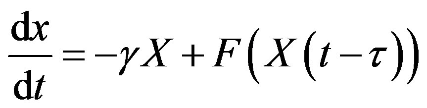
where 𝜏 is the average length of time required to go through the compartment (time delay). Typically, F is taken to be a monotone decreasing function of X to mimic the negative feedback loops of the system.
2.2.2. DDE with Distributed Delays
Delays arise in biological systems because of properties inherent to the different processes. Although constant delays may be an excellent approximation of the time event involved, one might want to account for the distribution of time delay. Indeed, in a real system, it is much more likely that events related to the delay are distributed with a density that is not a delta function. A distribution of delays is then be more appropriate and the DDE becomes an integro-differential equation of the form
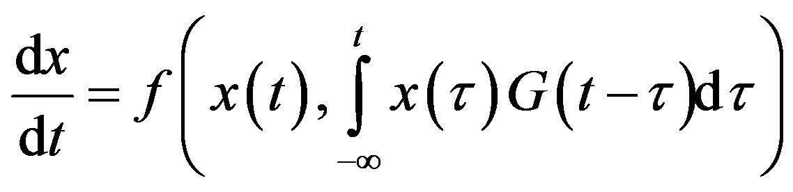 (3)
(3)
The density G(u) of the distribution function is referred to as he memory function or the kernel and is normalizedi.e. 
This type of model can also be interpreted as allowing for a stochastic element in the duration of the delay. Also, we will see that for some densities G(u), it can be equivalently viewed as a system of ordinary differential equations.
2.2.3. DDE with State-Dependent Delays
Another type of delay differential equation occurs when the delay depends on a state variable. For example, one could imagine that the maturation time for a blood cell depends on the amount of growth factor in the circulation as, for example, is the case with the maturation time of neutrophil precursors in humans. An example of a model with a state-dependent delay can be found in [14,18,19], but it is fair to say that models of hematopoietic regulation with state dependent delays have not appeared because of the paucity of data for the analytic variation of delays with respect to state variables.
2.3. ODE Models
Delay differential equations naturally arise in modelling biological systems. However, since DDEs are infinitedimensional systems, they are difficult to analyze and handle numerically. For some forms of delays, the socalled linear chain trick enables the model to be written as an equivalent finite-dimensional system of ordinary differential equations. Next, we present a simple example of this method which is a specific example of the more general considerations of [1]. Consider the following DDE system with a distributed delay:
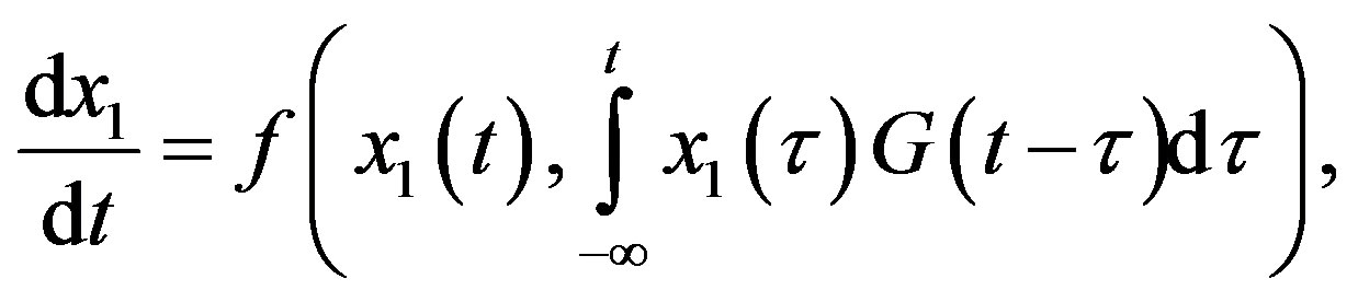
with the special choice of the density of the gamma distribution for the memory function
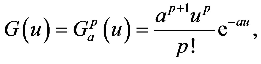
where “a” is a positive number and “p” is a positive integer or zero. Note that the function G(u) has a maximum at u = p/a and that, as a and p increase, keeping p/a fixed, the kernel approaches a delta function and the distributed delay approaches the discrete time delay with 𝜏 = p/a. Moreover, it is clear that the following three properties are satisfied:
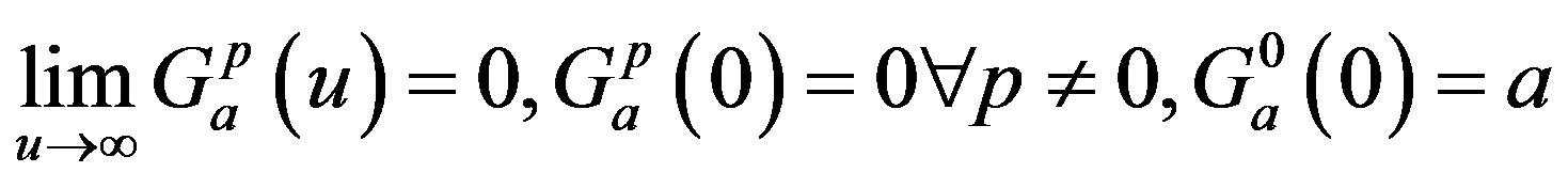
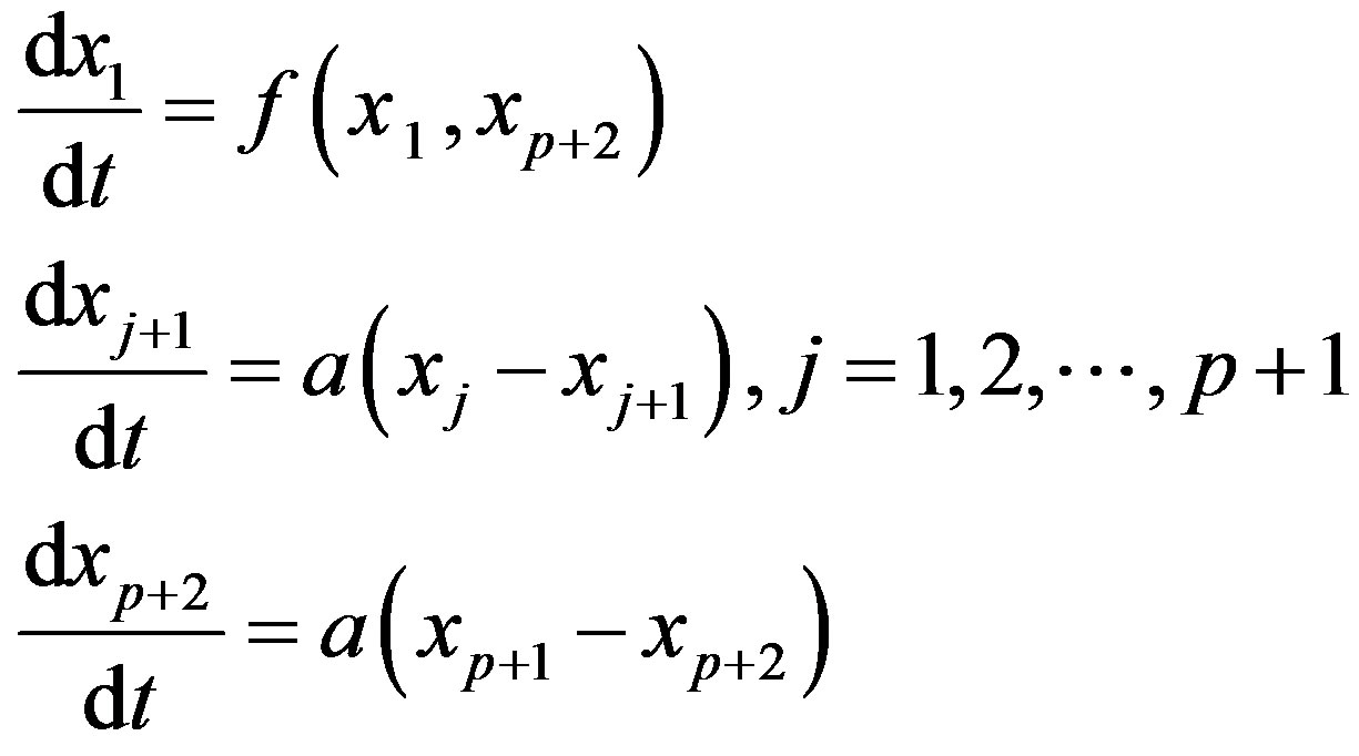
The central idea of the method is to replace the distributed delay by an extension of the set of variables. Define p + 1 new variable as
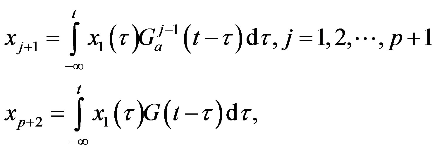
Then, using the properties of G one can show that these new variables satisfy a sequence of linear ODE. Solving the following system is thus equivalent to solving the DDE problem (3), given that the new variables are given appropriate initial values:
The linear chain trick could be useful for numerical computations since it reduces the problem to an ODE system, for which several numerical methods are available. However, this method cannot be used for all sorts of delays, see [1]. Within a hematological context, [13] were unable to use this technique in their model of neutrophil production because the estimated value of p in the experimentally determined distribution of delays was not an integer. Other models [20] have used constructs somewhat analogous to the system. Introducing a delay in a system could be thought of as a way of including age-structure in the model. For instance, one could think of setting up a detailed model in which the population dynamics is described by several maturation stages. If enough detail is known about the time spent in each stage, one could then associate a differential equation with each stage. However, detailed data such as these are often not available. Alternatively, one could lump together all the stages and reduce the model to only one DDE where the delay is the total maturation time. Another option would be to use partial differential equations, as we will discuss in the next section.
2.4. Age-Structured Models
We now present a typical PDE model used in several applications. Indeed, a cell starts from the hematopoietic stem cell and then its progeny go through a number of stages before being released into the circulation. One could model this process by associating a partial differential equation for the cell density function with each stage, which describes the population in the compartment as a function of the variables age a and time t. The model also contains feedback control elements that regulate the release of cells from one compartment to the other. The number of compartments depends on the data available which determines the maximum level of detail appropriate for the model. For instance, a model of erythropoiesis could have one compartment for each recognizable stage of erythrocytes precursors, or alternatively merge some of the compartments together and thus reduce the model dimensions. In the following, we will present some results using only a generic compartment. The treatment for a larger model is the same. We then show that by partial integration we can express this problem as a delay differential equation model. Age-structured models provide a means of understanding the regulation of hematopoiesis. Examples in the literature can be found in [2].
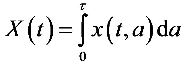
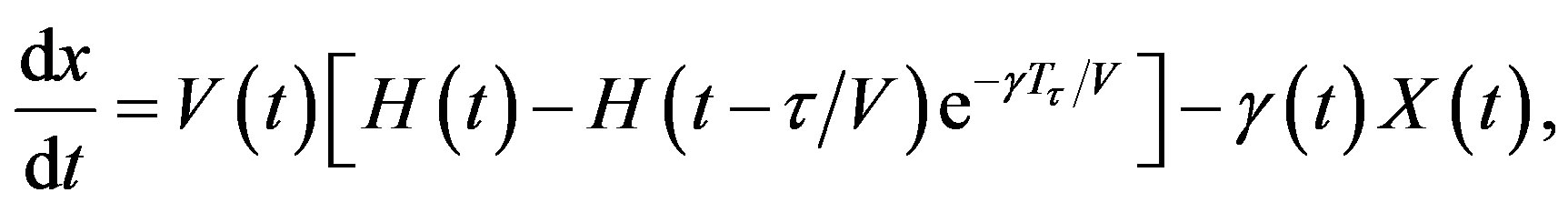
Let x(t, a) be the cell density at time t and age a in a generic compartment. We assume that cells disappear (die) at a rate (t). We also assume that the cells in the compartment age with a velocity V(t) and that a cell enters a compartment at age a = 0 and exits this compartment at age a = 𝜏. Therefore, the equation satisfied by x(t, a) is an time-age equation:
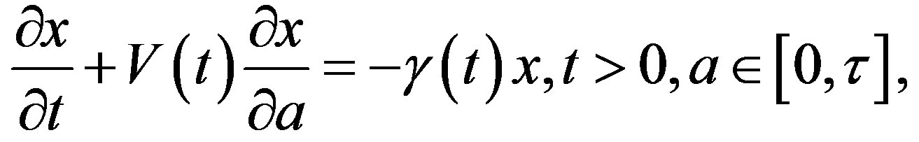
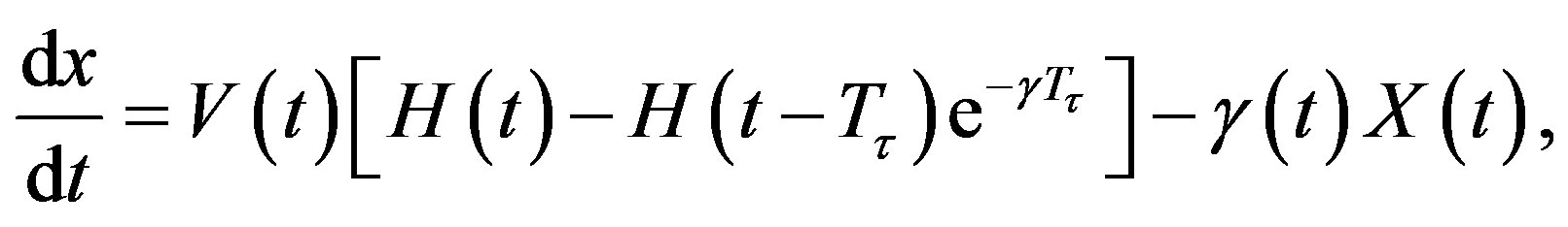
The right hand side in this equation represents the rate at which cells in the age interval a to a + 𝛿a disappear at time t. To represent the manner in which new cells enter the compartment, we define the boundary condition (B.C.) x(t, 0) = H(t). Finally, to fully represent the problem, we specify the initial condition (I.C.)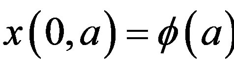 . We show that by partial integration of equation, we can reformulate this problem as a delay differential equation. Using the method of characteristics, we obtain the following delay differential equation:
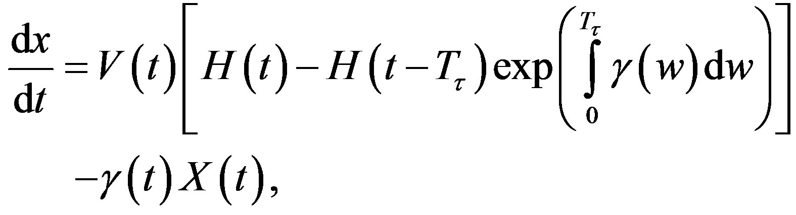 (4)
(4)
where X(t) is the total number of cells
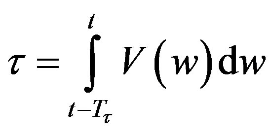
 and Tτ satisfies
 . Note that if is a constant, Equation (4) reduces to
In addition, if the aging velocity is constant , we have that Tτ satisfies
which implies that Tτ = 𝜏/V. Hence, if γ and V are constant, we obtain a delay differential equation with constant delay:
3. Model Input Function
We must also specify an input function I(t) that represents the subcutaneous G-CSF injections [14,21,22]. We assume that this input is brief in duration, and that the total amount of G-CSF added corresponds to the desired dosage, namely:
Note that if 𝜎 is small, a Gaussian-like input approximates a Dirac 𝛿-function, and we can write

Therefore to simulate periodic injections, we let
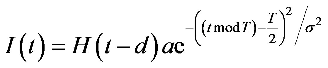
where H(t) denotes the Heaviside step function
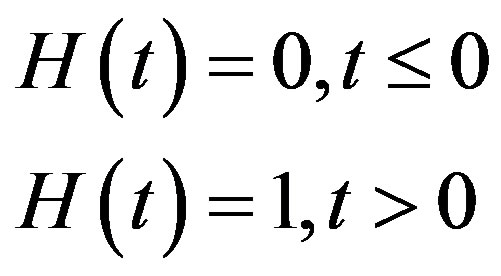
The day on which treatment is initiated is denoted by d, and the Heaviside function simply turns the injections on. The term “t mod T” ensures periodicity, and we require that  so that the approximation to the integral remains valid. Finally, we ensure that Equation (3) holds by choosing the parameter that a
  = dosage. It remains only to describe how the G-CSF acts on the hematological portion of the model. Because we believe from previous modeling efforts that AN, 𝛾S, and
  are the parameters that need to change under G-CSF, we model G-CSF injections as causing fluctuations in these three parameters:
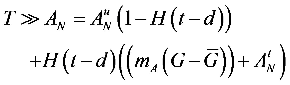
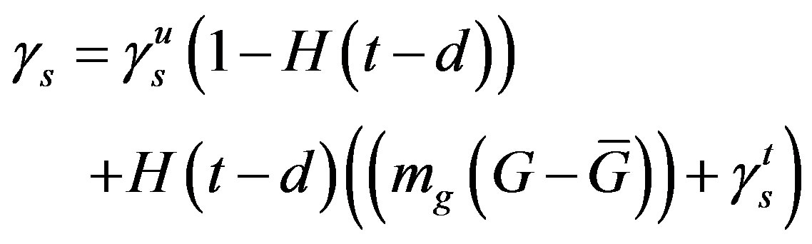
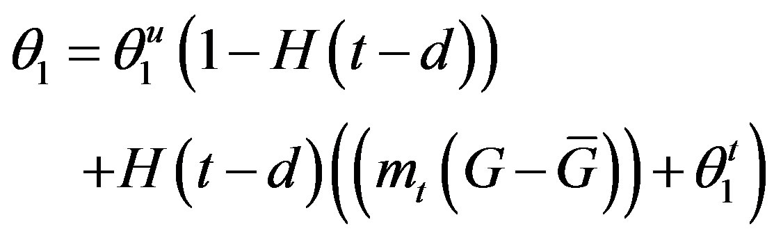
The superscripts “t” and “u” respectively indicate values corresponding to values that, in the model without the dynamics of G-CSF, match treated and untreated data respectively. The parameters mA, mg, and mt are slopes that specify how much AN, γS, and  change in response to a given change in G-CSF concentration,
  is the average G-CSF concentration for each data set. These were computed using the G-CSF model alone, and using the average neutrophil levels in each data set.
4. Results
The parameter sets for the first three dogs are given in the first three columns of Table 1 in the model. In each case, we found that the neutrophil amplification increases substantially under G-CSF treatment, as does the rate of stem cell apoptosis, and the differentiation into the neutrophil line. We therefore predict similar changes for the remaining dogs (see the four last columns in Table 1). There is some redundancy in the model, in that increasing the neutrophil amplification and the differentiation into the neutrophil line from the stem cells has similar effects.
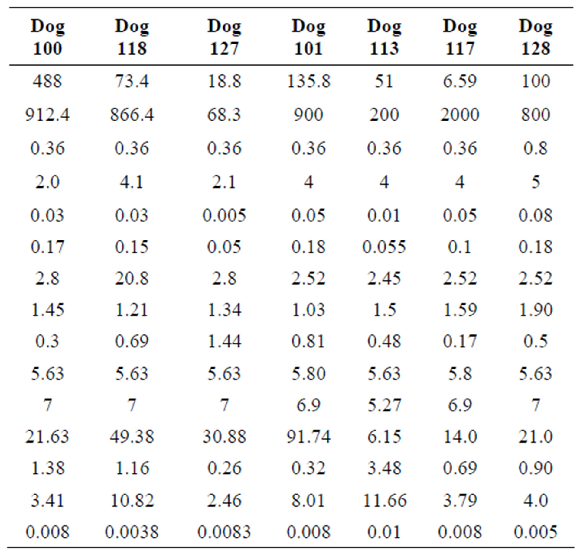
Table 1. Parameters used for computation for each dog.
This is not unexpected, since the primary effect of both changes is to raise neutrophil levels. Figure 1 shows the fit of the untreated and treated data for Dogs 100, 118 and 127. This confirms that the new model, with the G-CSF coupled to the cell population dynamics, is capable of reproducing the data. The least squares differences between the FFT analysis and the data were not significantly less than the reported values. Figure 1 shows the data and analysis for the other four dogs (Dogs 101, 113, 117 and 128), again with daily treatment. Recall that these were the estimated, not fitted, values for the treated parameters and note the quality of the fits. Thus, we are able to match observed data without automated parameter fitting based simply on an examination of the treated data and the parameter changes for Dogs 100, 118 and 127. For each dog, we performed simulations comparing daily treatment, treatment every other day, and every three days. We find that particularly for Dogs 100, 101, 118 and 127, changing the period of the treatment can significantly affect the nature of the oscillations. It shows the results of treating Dog 118 every other day, rather than every day. We have also explored the effects of changing the time at which the treatment is initiated. In most cases, this did not significantly change the long-term behavior. However, for Dog 127 the amplitude of the oscillations was significantly reduced when the treatment was initiated in the latter half of the cycle. More specifically, measured from day 1, we find that smaller oscillations occur if treatment is initiated on day 8 or afterwards, or on days 2 or 5 (see Figure 1). When treatment was initiated on other days, larger oscillations in the model resulted. It should also be noted that increasing the G-CSF dosage in the model sometimes helped to stabilize oscillations (Dog 127), but in several cases (Dogs 100, 128 and 101) a dosage increase from 5 μg/kg to a dosage in the range 15 - 25 μg/kg caused some FFT analysis to fail. In that analysis, the differentiation rate out of the stem cells was so high, and the apoptosis rate in the stem cells was so high, that the stem cell population was no longer able to maintain itself. For the other dogs, there was always a dosage that was sufficiently high to terminate the FFT analyze, but it was sometimes a factor of 10 higher than the actual dosage given (see Table 1).
5. Parameter Estimation
In this parameter estimation analysis we further present the main compartment, as well as the G-CSF compartment in decreasing bounded functions [3,13,19].
 (5)
(5)
We take  = 0.04 day–1 and
  = 0.18 day–1 from the Table 1 and Equation (5) we get
  = 0.018.
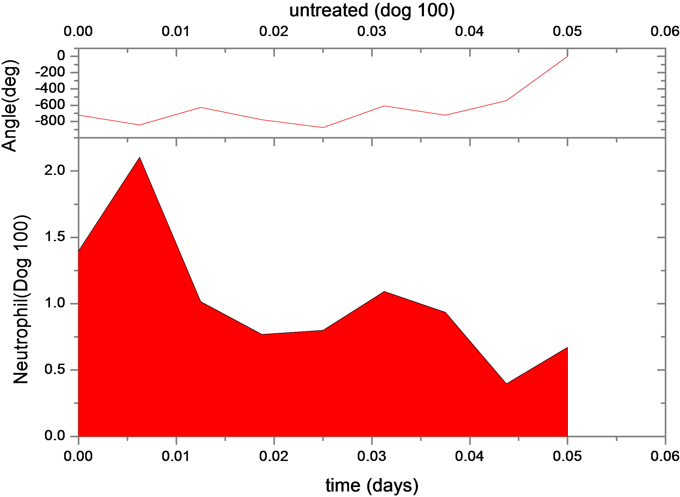
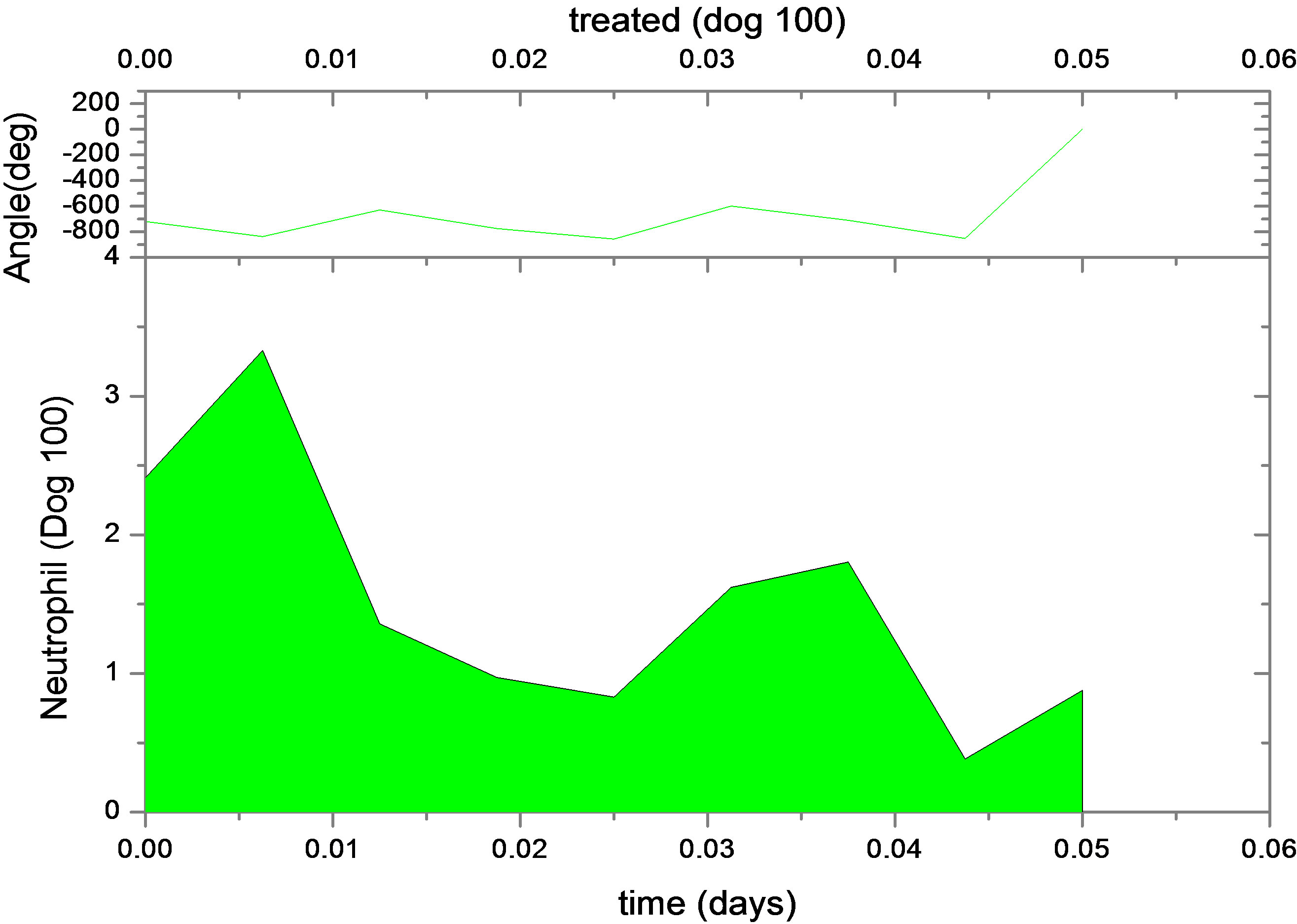
Figure 1. Continuous neutrophil data and analyze for Dogs 100, 118, 127, 101, 113, 117 and 128. The upper figure shows untreated data (red) and fit (normal area). The lower figure shows treated data (green) and analyze for dogs under daily G-CSF treatment. The calculations were obtained using parameters resulting from the FFT analysis method. Neutrophil units are 108 cells·kg−1.
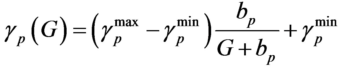 (6)
(6)
Similarly  = 0.27 (range 0.27 - 0.45), we take
= 0.27 and  = 0.42 from the Table 1, and Equation (6)
we get  = 0.42.
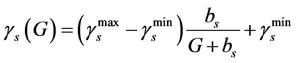
 (7)
(7)
Similarly  = 0.05 (range 0.01 - 0.20).
  = 0.27 (range 0.27 - 0.45), we take
  = 0.27 and
  =0.42, and Equation (7) we get
  = 0.42. Where
  and
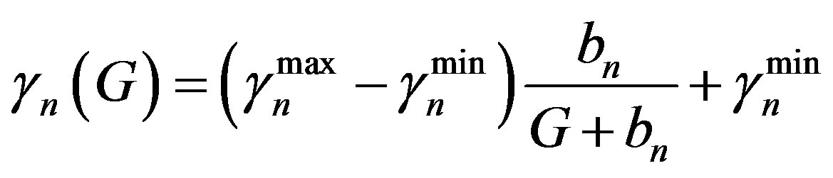
and  are the minimum and maximum values for the apoptosis rates (I = s, p, n) and bi is the control the steepness of the function (see Table 1). The values are bs = 0.01, bp = bn = 0.05 (or) bs = 0.01, bp = bn = 1 and G = 0.
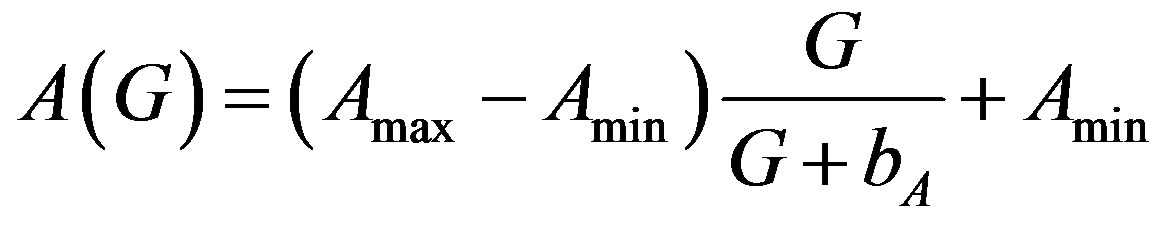
5.1. Amplification Factor A(G)
 (8)
(8)
From (8) we get,  = 20972 (100 days) and
= 655 (100 days),  = 0.35 (or)
  = 1.05. Ranges =
216 × 102 (655) to 218.3 × 10² (3700). Lower values of  is lead to higher ANC responses.
5.2. Differentiation Rate from Stem Cell
 , f0 = 0.40 day–1,
  = 0.36 × 10⁸
cells/kg, we take w = 6,  = 2399887.161. If w decreases, then
  increases.
5.3. Reentry into Stem Cell Proliferative Phase
where k0 = 8 day–1,  = 0.3 × 10⁶ cell/kg, we take s = 0.008, β(s) = 1. A number of parameters are to be estimated in this analysis. We require estimate of the transfer rates KT and KB, the volume VB, and the parameters α and γG, which gives the clearance rate of G-CSF from the blood stream. Here KT = 0.05 (calculated value), KB = 0.25, γ = 0.05 (calculated value), VB = 76, X = 0.1. The clearance rate is t1/2 = In2/(αN + γ). Hence it lies between 0.015 < α < 0.03 kg/hr.
6. Discussions
We used data on seven grey collies generously supplied by Dr. David C. Dale (University of Washington School of Medicine, Seattle) and previously analyzed in [16,17]. It is used to detect periodicity in the blood counts before and during treatment with G-CSF. Data for neutrophils, erythrocytes and platelets were available both for untreated dogs as well as dogs receiving daily G-CSF. We have developed a mathematical model that couples the pharmacokinetics of G-CSF to the hematopoietic stem cell, neutrophil, platelet and erythrocyte dynamics [23- 25]. It consists of 4 delay differential equations each describing the time evolution of one of the cell types. The G-CSF compartment adds 10 parameters, which are estimated from the literature (see Table 1). A FFT analysis method was used to minimize the least squares difference between the analysis and the data. Both the platelet and neutrophil counts were matched for dogs with untreated cyclical neutropenia, and for dogs undergoing daily treatment with G-CSF injections. For three of these, we used the FFT analysis procedure to minimize the least squares difference between the simulation and the treated data, changing only the three most critical parameters. We then estimated, without fitting, the treated parameters for the remaining 4 dogs. It determined both the untreated and treated parameter values we are in a position to use FFT to explore the effects of different treatment strategies [26-30].
We have developed a model which is called “hematopoietic” system. It includes pharmacokinetic model of G-CSF. It is dynamics in tissue and in circulation. This model helps us to account for the feature of untreated and G-CSF treated, data for dogs with cyclical neutropenia. This is accomplished by parameters for 3 or 4 dogs. There was an increase in the rate of apoptosis in the stem cell compartment during G-CSF treatment. Therefore, fit observed data for cyclical neutropenic dogs and human beings are treated by G-CSF model. During G-CSF treatment there is an increase in neutrophil amplification.
The treatment schedules indicated that changing the period from daily to other day, and then to third day almost change the nature of the oscillations. G-CSF is costly. It causes undesirable side effects [3,31,32]. It is possible to this option further in humans. We found in one case that changing the time of onset of treatment results in much smaller amplitude oscillations in the treated FFT analysis. It had more effects on the oscillations than did changing the dosage was not viable for an analysis. It is frequently led to the termination of the FFT rather than the stabilization of oscillations.
The observed data are highly viable from one dog to another. The stimulations can be individualized. This presents the possibility of using “real time” data for model analysis. It makes predictions about the effects of different treatment schedules. Earlier findings revealed different behavior that would result from different GCSF treatment schedules [33,34]. Our model substantiate that the quantities effects the realistic G-CSF dynamics and yielding analysis that are directly comparable to observed data. Our central result revealed in the G-CSF model is significant. The changing time of treatment initiation or the period of treatment may result in equally good or better, long-term outcomes. It may require less G-CSF. These changes would be practical to implement in treatment and less G-CSF is required. It would reduce the risk, of side effects as well as the cost of treatment.
7. Conclusion
In our analysis we widely discussed hematological processes and related dynamical diseases. It provides an understanding into hemotopoietic regulatory systems. It helps us clinical treatment of G-CSF. Further, we have examined different G-CSF treatment and methods for CN using a model approach. Therefore we used two dimensional DDE models namely, neutrophils and stem cells. Two sets of parameters CN and G-CSF have been illustrated and three parameters were modified to the effects of treatment. These parameters are amplification, rate of apoptosis and the maximal rate of differentiation from the hematopoietic stem cells and the neutrophil line. We found that a large neutrophil become a greater level and followed by a deep position or a smaller ANC (Absolute Neutrophil Count) in high level. It remains stable and does not go to lower levels. There is a change among patients in several parameters. It may sometimes influence treatment.
REFERENCES
- M. Adimy and F. Crauste, “Global Stability of a Partial Differential Equation with Distributed Delay Due to Cellular Replication,” Nonlinear Analysis: Theory, Methods & Applications, Vol. 54, No. 8, 2003, pp. 1469-1491. doi:10.1016/S0362-546X(03)00197-4
- S. Balamuralitharan and S. Rajasekaran, “A Mathematical Age-Structured Model on Aiha Using Delay Partial Differential Equations,” Australian Journal of Basic and Applied Sciences, Vol. 5, No. 4, 2011, pp. 9-15.
- S. Balamuralitharan and S. Rajasekaran, “A Mathematical Age-Structured Model on CN Using Delay Partial Differential Equations,” Proceedings of the International Conference on Emerging Trends in Mathematics and Computer Applications. MEPCO Schlenk Engineering College, Sivakasi, 16-18 December 2010, pp. 183-187.
- J. Bélair, M. C. Mackey and J. M. Mahaffy, “Age-Structured and Two-Delay Models for Erythropoiesis,” Mathematical Biosciences, Vol. 128, No. 1-2, 1995, pp. 317-346. doi:10.1016/0025-5564(94)00078-E
- S. Bernard, J. Belair and M. Mackey, “Oscillations in Cyclical Neutropenia: New Evidence Based on Mathematical Modeling,” Journal of Theoretical Biology, Vol. 223, No. 3, 2003, pp. 283-298. doi:10.1016/S0022-5193(03)00090-0
- A. Beuter, L. Glass, M. C. Mackey and M. S. Titcombe, “Nonlinear Dynamics in Physiology and Medicine,” Springer-Verlag, New York, 2003.
- S. P. Blythe, R. M. Nisbet and W. S. C. Gurney, “The Dynamics of Population Models with Distributed Maturation Periods,” Theoretical Population Biology, Vol. 25, No. 3, 1984, pp. 289-311. doi:10.1016/0040-5809(84)90011-X
- T. Cohen and D. P. Cooney, “Cyclical Thrombocytopenia: Case Report and Review of Literature,” Scandinavian Journal of Haematology, Vol. 16, 1974, pp. 133-138.
- C. Colijn and M. Mackey, “A Mathematical Model of Hematopoiesis: II. Cyclical Neutropenia,” Journal of Theoretical Biology, Vol. 237, No. 2, 2005, pp. 133-146. doi:10.1016/j.jtbi.2005.03.034
- C. Colijn, A. C. Fowler and M. C. Mackey, “High Frequency Spikes in Long Period Blood Cell Oscillations,” Journal of Mathematical Biology, Vol. 53, No. 4, 2006, pp. 499-519. doi:10.1007/s00285-006-0027-9
- D. C. Dale and W. P. Hammond, “Cyclic Neutropenia: A Clinical Review,” Blood Reviews, Vol. 2, No. 3, 1988, pp. 178-185. doi:10.1016/0268-960X(88)90023-9
- D. Fargue, “Reductibilite des Systemes Hereditaires,” International Journal of Non-Linear Mechanics, Vol. 9, No. 5, 1974, pp. 331-338. doi:10.1016/0020-7462(74)90018-3
- C. Foley and M. Mackey, “Dynamic Hematological Disease: A Review,” Journal of Mathematical Biology, Vol. 58, No. 1-2, 2008, pp. 285-322.
- C. Foley, S. Bernard and M. Mackey, “Cost-Effective G-CSF Therapy Strategies for Cyclical Neutropenia: Mathematical Modelling Based Hypotheses,” Journal of Theoretical Biology, Vol. 238, No. 4, 2006, pp. 754-763. doi:10.1016/j.jtbi.2005.06.021
- P. Fortin and M. C. Mackey, “Periodic Chronic Myelogenous Leukemia: Spectral Analysis of Blood Cell Counts and Etiological Implications,” British Journal of Haematology, Vol. 104, No. 2, 1999, pp. 336-245. doi:10.1046/j.1365-2141.1999.01168.x
- D. Guerry, D. Dale, D. C. Omine, S. Perry and S. M. Wolff, “Periodic Hematopoiesis in Human Cyclic Neutropenia,” Journal of Clinical Investigation, Vol. 52, No. 12, 1973, pp. 3220-3230. doi:10.1172/JCI107522
- W. P. Hammond, T. H. Price, L. M. Souza and D. C. Dale, “Treatment of Cyclic Neutropenia with Granulocyte Colony Stimulating Factor,” The New England Journal of Medicine, Vol. 320, 1989, pp. 1306-1311. doi:10.1056/NEJM198905183202003
- C. Haurie, M. C. Mackey and D. C. Dale, “Cyclical Neutropenia and Other Periodic Hematological Diseases: A Review of Mechanisms and Mathematical Models,” Blood, Vol. 92, 1998, pp. 2629-2640.
- C. Haurie, D. C. Dale, R. Rudnicki, and M. C. Mackey, “Modeling Complex Neutrophil Dynamics in the Grey Collie,” Journal of Theoretical Biology, Vol. 204, No. 4, 2000, pp. 504-519. doi:10.1006/jtbi.2000.2034
- T. Hearn, C. Haurie and M. C. Mackey, “Cyclical Neutropenia and the Peripherial Control of White Blood Cell Production,” Journal of Theoretical Biology, Vol. 192, No. 2, 1998, pp. 167-181. doi:10.1006/jtbi.1997.0589
- M. Horwitz, K. F. Benson, Z. Duan, F.-Q. Li and R. E. Person, “Hereditary Neutropenia: Dogs Explain Human Neutrophil Elastase Mutations,” Trends in Molecular Medicine, Vol. 10, No. 4, 2004, pp. 163-170. doi:10.1016/j.molmed.2004.02.002
- E. A. King-Smith and A. Morley, “Computer Simulation of Granulopoiesis: Normal and Impaired Granulopoiesis,” Blood, Vol. 36, 1970, pp. 254-262.
- M. J. Koury, “Programmed Cell Death (Apoptosis) in Hematopoiesis,” Experimental Hematology, Vol. 20, 1992, pp. 391-394.
- M. Loeffler and K. Pantel, “A Mathematical Model of Erythropoiesis Suggests an Altered Plasma Volume Control as Cause for Anemia in Aged Mice,” Experimental Gerontology, Vol. 25, No. 5, 1990, pp. 483-495. doi:10.1016/0531-5565(90)90036-2
- N. MacDonald, “Time Lags in Biological Models,” Springer-Verlag, New York, 1978. doi:10.1007/978-3-642-93107-9
- M. C. Mackey, “Periodic Auto-Immune Hemolytic Anemia: An Induced Dynamical Disease,” Bulletin of Mathematical Biology, Vol. 41, 1979, pp. 829-834.
- M. C. Mackey and A. Rudnicki, “Global Stability in a Delayed Partial Differential Equation Describing Cellular Replication,” Journal of Mathematical Biology, Vol. 33, No. 1, 1994, pp. 89-109. doi:10.1007/BF00160175
- J. Mahaffy, J. Belair and M. Mackey, “Hematopoietic Model with Moving Boundary Condition and State Dependent Delay: Applications in Erythropoiesis,” Journal of Theoretical Biology, Vol. 190, No. 2, 1998, pp. 135- 146. doi:10.1006/jtbi.1997.0537
- I. Ostby, G. Kvalheim, L. S. Rusten and P. Grottum, “Mathematical Modeling of Granulocyte Reconstitution after High-Dose Chemotherapy with Stem Cell Support: Effect of Posttransplant G-CSF Treatment,” Journal of Theoretical Biology, Vol. 231, No. 1, 2004, pp. 69-83. doi:10.1016/j.jtbi.2004.05.010
- T. H. Price, G. S. Chatta and D. C. Dale, “Effect of Recombinant Granulocyte Colony Stimulating Factor on Neutrophil Kinetics in Normal Young and Elderly Humans,” Blood, Vol. 88, 1996, pp. 335-340.
- I. Roeder, “Quantitative Stem Cell Biology: Computational Studies in the Hematopoietic System,” Current Opinion in Hematology, Vol. 13, No. 4, 2006, pp. 222- 228. doi:10.1097/01.moh.0000231418.08031.48
- S. I. Rubinow and J. L. Lebowitz, “A Mathematical Model of Neutrophil Production and Control in Normal Man,” Journal of Mathematical Biology, Vol. 1, No. 3, 1975, pp. 187-225. doi:10.1007/BF01273744
- M. Santillan, J. Mahaffy, J. Belair and M. Mackey, “Regulation of Platelet Production: The Normal Response to Perturbation and Cyclical Platelet Disease,” Journal of Theoretical Biology, Vol. 206, No. 4, 2000, pp. 585-603. doi:10.1006/jtbi.2000.2149
- S. Balamuralitharan and S. Rajasekaran, “Analysis of G-CSF Treatment of CN Using Fast Fourier Transform,” Salt Lake, Kolkata, 2011. http://www.imbic.org/forthcoming.html
NOTES
*Corresponding author.