American Journal of Operations Research
Vol.06 No.02(2016), Article ID:64279,8 pages
10.4236/ajor.2016.62014
Forecasting Spare Parts Demand Using Statistical Analysis
Raghad Hemeimat, Lina Al-Qatawneh, Mazen Arafeh, Shadi Masoud
Department of Industrial Engineering, University of Jordan, Amman, Jordan

Copyright © 2016 by authors and Scientific Research Publishing Inc.
This work is licensed under the Creative Commons Attribution International License (CC BY).
http://creativecommons.org/licenses/by/4.0/


Received 31 December 2015; accepted 5 March 2016; published 8 March 2016
ABSTRACT
Spare parts are very essential in most industrial companies. They are characterized by their large number and their high impact on the companies’ operations whenever needed. Therefore companies tend to analyze their spare parts demand and try to estimate their future consumption. Nevertheless, they face difficulties in figuring out an optimal forecasting method that deals with the lumpy and intermittent demand of spare parts. In this paper, we performed a comparison between five forecasting methods based on three statistical tools; Mean squared error (MSE), mean absolute deviation (MAD) and mean error (ME), where the results showed close performance for all the methods associated with their optimal parameters and the frequency of the spare part demand. Therefore, we proposed to compare all the methods based on the tracking signal with the objective of minimizing the average number of out of controls. This approach was tested in a comparative study at a local paper mill company. Our findings showed that the application of the tracking signal approach helps companies to better select the optimal forecasting method and reduce forecast errors.
Keywords:
Forecasting, Spare Parts, FSN, Moving Average, Exponential Smoothing, Tracking Signal

1. Introduction
In industries that have a production system, the product goes through multiple processes and undergoes several machines in order to get the final product intended. All machines require maintenance and spare parts. Spare parts must be available whenever needed in order to prevent the whole production line from being stopped and thus affecting the production rates. Therefore, companies started to develop their own spare parts management system in order to analyze and manage any spare parts related issues.
Different quantitative and qualitative forecasting methods are applied to predict the future demand of spare parts in order to consistently ensure their availability. Time series methods are considered the most common and reliable quantitative methods. In time series forecasting, there is a major difference between forecasting the demand of finished goods and forecasting the demand of spare parts. That’s clearly noticed in literature [1] .
Some traditional forecasting techniques might not be applicable for spare parts. Spare parts forecasting poses a large challenge for all forecasters. The reason is that the demand is stochastic and a big proportion of the demand data is zero for several periods of time resulting on having inaccurate results.
Classifications of parts can serve for accurate forecasts. Classification can be based on the importance, frequency or cost of parts or even a combination of different criteria. This can assure that the essential or frequently needed parts are always available. However, storing unessential or rarely used parts can add unwanted costs. Therefore, it is important to control the quantities of spare parts without risking the stoppage of the production line. Achieving this will result in maximizing the company’s service level and eliminating unnecessary high inventory costs.
This research is motivated by the problem of forecasting spare parts demand at a local paper mill company where spare parts of different types are stocked to ensure their availability and to avoid any shortcuts in the production line when damages occur; the company tends to analyze its demand and try to estimate its future consumption roughly depending on experience. There is a variety of forecasting techniques that can be used by the company, yet, no one of them is best for all items and situations. One way of improving the forecast accuracy is to focus on reducing the forecast error. Therefore, one of the approaches used in selecting a forecasting method from several ones is to choose the one with the best performance based on certain calculated performance measures. Some of these performance measures that have been suggested in literature are: mean error (ME), mean squared error (MSE) and mean absolute deviation (MAD). In this paper, we will suggest an alternative approach to select the forecasting method with the least forecast error.
The remainder of this paper is organized as follows. Section 2 gives an overview of the relevant literature. The classification of spare parts based on demand is described in Section 3. In Section 4, the various forecasting methods used in this study are introduced. Section 5 summarizes the comparative analysis conducted on our case study and its results. The suggested alternative approach is discussed thoroughly in Section 6. Finally, the conclusion of our research along with its implications is presented in Section 7.
2. Relevant Literature
Forecasting demand has been an important issue for many years. General guidelines and overview on spare parts management were summarized by Kennedy et al. [2] . Moreover, many forecasting methods were discussed intensively in literature starting with Croston who showed that both moving average and exponential smoothing do not perform well for intermittent demand [3] . Later, a number of extensions and improvements have been made to the method, notably by Syntetos and Boylan [4] where they showed that the original Croston method is biased. Then they then suggested an adjustment for this in a following paper [5] . Finally, Teunter et al. [6] [7] proposed an improvement on Croston’s method that suggests to update the demand probability instead of the demand interval.
Bootstrapping methods for forecasting were also included in literature which offer a non-parametric alternative for forecasting. The most well-known bootstrapping methods are those of Willemain et al. [8] and Porras and Dekker [9] .
Papers relevant to our work contained case studies on forecasting spare parts demand for various industries (aircrafts, automotive, etc). For example, Romeijnders et al. suggested a two-step method for forecasting spare parts demand using information on component repairs [10] . Another case for Şahin et al. who applied Croston’s method integrated with an artificial neural network to forecast spare parts demand of an aviation company [11] . Their proposed forecasting method served in reducing inventory costs and eliminating the risk of keeping planes on the ground. In a recent research, Kontrec et al. proposed a reliability model to evaluate the characteristics of aircraft consumable parts in order to plan and control non repairable spare parts forecasting in an aircraft maintenance system [12] .
3. Data Description
The data set contains information on over 100,000 ordered spare parts at the paper mill company during the period from October 2013 till January 2015 [13] . Each spare part data includes the item code, item description, order date and the issued quantity. The total number of spare parts item used is 1223. A monthly forecast will be done. Using the fast-slow-nonmoving (FSN) analysis; spare part items were classified into three categories; fast moving items, slow moving items and non-moving items. The classification is conducted based on the monthly demand of spare part. Table 1 shows the results of the classification.
4. Forecasting Methods
In this section, an overview of the considered forecasting methods is presented. The methods and their abbreviations are shown in Table 2. The used notations and their description with abbreviations of related methods between brackets are shown in Table 3.
Five different time series forecasting methods were used in the study as listed below:
1) Moving average forecast (MA).
Essentially, moving average method tries to estimate the next period’s value by averaging the value of the last couple of periods immediately prior. The moving average forecast (MA) is the mean of the previous N months, where N is the number of months used in the forecast [14] .
 (1)
(1)
2) Exponential smoothing forecast (ES)

Table 1. Results of FSN classifications.
Table 2. The forecasting methods and their abbreviations.
Table 3. Notation used and their description.
Exponential smoothing is simply an adjustment technique which takes the previous period’s forecast, and adjusts it up or down based on what actually occurred in that period [14] . It accomplishes this by calculating a weighted average of the two values.
 (2)
(2)
where  is the smoothing constant.
3) Croston’s forecasting method (CR)
The Croston’s method is a forecast strategy for products with intermittent demand. This method consists of two steps. First, separate exponential smoothing estimates are made of the average size of a demand. Second, the average interval between demands is calculated. This is then used in a form of the constant model to predict the future demand, as will be shown later [3] .
 (3)
(3)
 (4)
(4)
where  and the Croston forecast is
 (5)
(5)
4) Syntetos-Boylan approximation (SBA)
Syntetos and Boylan showed that Croston’s method is positively biased. To approximately correct for that bias, they proposed to deflate the Croston forecast by a factor (α/2). Thus, this method is a modified version of Crostons forecasting method [4] [5] .
 (6)
(6)
5) Teunter-Syntetos-Babai forecasting method. (TSB)
This model is another modification of Croston method proposed by Teunter et al. [6] . The difference between these methods is that the Croston’s method updates demand interval, the TSB method updates the demand probability (inverse of demand interval). In other words, while, TSB model is using separate simple exponentially smoothed estimates of the demand probability and the demand size. Since demand probability can be updated in every period, this method is unbiased and can be used to estimate the risk of obsolescence (although in fact it cannot prevent obsolescence completely) as well as relate forecasting to other inventory decisions. This method achieves a high flexibility by using different smoothing constant for demand size and demand probability.
This probability and the demand size are updated,
 (7)
(7)
 8)
8)
 (9)
(9)
5. Running the Data Using VBA Macros and Results
Due to the large number of items and the calculations needed to be done, VBA excel macros were used to execute the above forecasting methods on the available spare parts data in order to have accurate results with fewer errors and to reduce repetitive work. Six macros were created, one of which was used to automate the data entry and the recording process of the forecasts’ results. The other five macros were used to find the best parameters for each forecasting method. It is worth mentioning that several values of the forecasting parameters (α, β) for all methods were tested in a sensitivity study and the parameters that gave the least error value were selected.
This section shows the comparative results for the forecasting methods used for the three spare parts categories. The comparison is done using the following performance measures: the mean error (ME), the mean squared error (MSE) and mean absolute deviation (MAD). The (ME) estimates the bias of the forecasting method, the (MSE) and the (MAD) are estimators of the variance. The main difference between the MSE and MAD is that the MSE is more sensitive to outliers. Noting that in the graphical representation of the comparison, the root mean squared error (RMSE) is used instead of MSE.
5.1. Fast Moving Items
Table 4 shows the parameters obtained to compare between the forecasting methods for the fast moving items. Figure 1 shows the performance measures obtained for the five forecasting methods for the fast moving items. The results show that the reliance on RMSE instead of MAD has small impact on the comparison between methods. The SBA method gives the lowest RMSE with value equals to 6.385. However it gives high bias through ME value of −0.815. The TSB method gives the second lowest RMSE value with a value equals to 6.460. TSB gives −0.508 ME value which is better than SBAs’ ME value. However, it is considered a low ME value compared to the remaining three methods. MA and ES methods show close error measures values. Lastly, the CR method shows the poorest RMSE performance with a value equal to 6.661.
5.2. Slow Moving Items
Table 5 shows the parameters obtained to compare between the forecasting methods for the slow moving items.
Table 4. Optimal parameters for fast moving items.
Table 5. Optimal parameters for slow moving items.

Figure 1. Performance measures for different methods (fast moving items).
Figure 2 shows the performance measures obtained for the five forecasting methods for the slow moving items. The TSB method gives the lowest RMSE with value equals to 0.867. It also gives the lowest ME with a value equals to −0.201. Not far from TSB, the SBA method gives the second lowest RMSE value with a value equals to 0.889. SBA gives ME equal to −0.150. Lastly, the ES method shows the poorest RMSE performance with a value equal to 1.139 and ME value equal to 0.010.
5.3. Non-Moving Items
Table 6 shows the parameters obtained to compare between the forecasting methods for the nonmoving items. Figure 3 shows the performance measures obtained for the five forecasting methods for the nonmoving items. The TSB method gives the lowest RMSE with value equals to 0.328. Also it gives the lowest ME value of −0.073. The MA method gives the second lowest RMSE with a value equals to 0.345. In addition, MA has the best bias performance with ME value equals to −0.006. Lastly, the CR method shows the poorest RMSE performance with a value equals to 0.396.
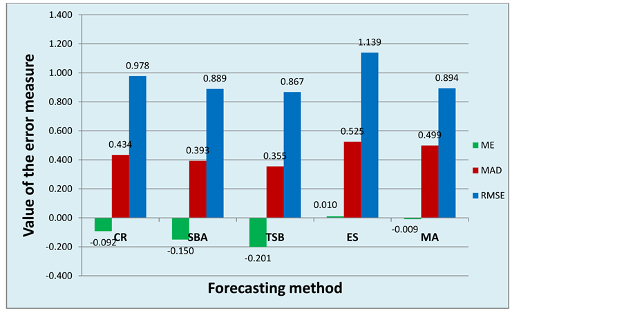
Figure 2. Performance measures for different methods (Slow moving items).

Figure 3. Performance measures for different methods (Non moving items).
6. Suggested Alternative Approach
Tracking Signal (TS) has been used as a measure of forecast accuracy. The benefit of using TS that it is an unbiased measure and can be used for any type of forecasting method. A tracking signal is calculated by dividing the most recent sum of forecast errors by the most recent estimate of MAD. Then, it is compared to the control limits; as long as the tracking signal is within these limits, the forecast is in control. One standard deviation is approximately equivalent to 1.25 MAD. So, a common boundary of 3 standard deviations is used (or 3.75 MAD); consequently, Control limits of ±4 were used.
 (10)
(10)
The suggested alternative approach combines the usage of traditional tracking signal approach with additional steps to find the best forecasting method and its parameters. The procedure included the following: first, for each spare part, the tracking signal for the corresponding time period (one month) was calculated. Then, it was compared to the assigned control limits. After that, the number of out of controls was counted per item for the whole time period (Oct 2013-Jan 2015). This was conducted for all fast moving items using VBA macro. Finally, the average of the out of control TS for all items is calculated.
This was applied to a range of values for the parameters (α, β) of each forecast; the parameters that gave the minimum average of the numbers of out of control TS were chosen and is shown in Table 7. Afterwards, a comparison was made for the five forecasting methods using the selected parameters as shown in Figure 4. The
Table 6. Optimal parameters for no-moving moving items.
Table 7. Optimal parameters for tracking signal approach.

Figure 4. Number of out of control Tracking Signals for different methods.
results show that MA method yields minimum average number of out of control TS with an average of 1.691. Not far from that, TSB and ES methods show good performance with an average of 1.868 and 1.836 respectively. In contrast, CR forecasting and SBA methods show poor performance with an average of 4.507 and 4.066 respectively. It is worth mentioning that this was applied for fast moving items only.
The results showed very close RMSE performance for all the five methods used. However, in the tracking signal method, there are three methods which outperformed the other methods. We can’t compare between the results of RMSE and TS approaches because the methods used different optimal parameters. For example, the parameters N (number of months in the moving average method) have noticeable difference between the two approaches; 10 for RMSE approach and 1 for TS approach. In addition, the results showed that the reliance on RMSE instead of MAD has small impact on the comparison between methods.
7. Conclusion
Maintaining sufficient stocks of spare parts is essential for any organization in order to quickly carryout repair operations and prevent the stoppage of production operations. The nature of spare parts demand, which is known to be lumpy and intermittent, leads to the consideration of different forecasting methods including: MA, ES, TSB, SBA and CR. Various methods are adopted in literature to compare between forecasting methods with the objective of minimizing the forecasting error. In this paper, through the case study, we have demonstrated the use of traditional tracking signal approach with additional steps to find the best forecasting method and its parameters. Our findings showed that the application of the proposed approach can help in selecting the optimal forecasting method in a better and more conclusive way compared to other methods that are also tested here in this paper. Case studies do not necessarily offer generalizable solutions. Therefore, future work can validate the usefulness of the proposed approach by applying it in different sectors.
Cite this paper
RaghadHemeimat,LinaAl-Qatawneh,MazenArafeh,ShadiMasoud, (2016) Forecasting Spare Parts Demand Using Statistical Analysis. American Journal of Operations Research,06,113-120. doi: 10.4236/ajor.2016.62014
References
- 1. Morris, M. (2013) Forecasting Challenges of the Spare Parts Industry. Journal of Business Forecasting, 32, 22-27.
- 2. Kennedy, W.J., Patterson, J.W. and Fredendall, L.D. (2002) An Overview of Recent Literature on Spare Parts Inventories. International Journal of Production Economics, 76, 201-215.
http://dx.doi.org/10.1016/S0925-5273(01)00174-8 - 3. Croston, J.D. (1972) Forecasting and Stock Control for Intermittent Demands. Operational Research Quarterly, 23, 289-303.
http://dx.doi.org/10.2307/3007885 - 4. Syntetos, A.A. and Boylan, J.E. (2001) On the Bias of Intermittent Demand Estimates. International Journal of Production Economics, 71, 457-466.
http://dx.doi.org/10.1016/S0925-5273(00)00143-2 - 5. Syntetos, A.A., Boylan, J.E. and Croston, J.D. (2005) On the Categorization of Demand Patterns. Journal of the Operational Research Society, 56, 495-503.
http://dx.doi.org/10.1057/palgrave.jors.2601841 - 6. Teunter, R. and Duncan, L. (2009) Forecasting Intermittent Demand: A Comparative Study. Journal of the Operational Research Society, 60, 321-329.
http://dx.doi.org/10.1057/palgrave.jors.2602569 - 7. Teunter, R.H., Syntetos, A.A. and Zied Babai, M. (2011) Intermittent Demand: Linking Forecasting to Inventory Obsolescence. European Journal of Operational Research, 214, 606-615.
http://dx.doi.org/10.1016/j.ejor.2011.05.018 - 8. Willemain, T.R., Smart, C.N. and Schwarz, H.F. (2004) A New Approach to Forecasting Intermittent Demand for Service Parts Inventories. International Journal of Forecasting, 20, 375-387.
- 9. Porras, E. and Dekker, R. (2008) An Inventory Control System for Spare Parts at a Refinery: An Empirical Comparison of Different Re-Order Point Methods. European Journal of Operational Research, 184, 101-132.
http://dx.doi.org/10.1016/j.ejor.2006.11.008 - 10. Romeijnders, W., Teunter, R. and van Jaarsveld, W. (2012) A Two-Step Method for Forecasting Spare Parts Demand Using Information on Component Repairs. European Journal of Operational Research, 220, 386-393.
http://dx.doi.org/10.1016/j.ejor.2012.01.019 - 11. Sahin, M., Kizilaslan, R. and Demirel, Ö.F. (2013) Forecasting Aviation Spare Parts Demand Using Croston Based Methods and Artificial Neural Networks. Journal of Economic & Social Research, 15, 1-21.
- 12. Kontrec, N.Z., Milovanovic, G.V., Panisc, S.R. and Milosevic, H. (2015) A Reliability-Based Approach to Nonrepairable Spare Part Forecasting in Aircraft Maintenance System. Mathematical Problems in Engineering, 2015, 1-7.
http://dx.doi.org/10.1155/2015/731437 - 13. Nuqul Tissues. (2015).
http://www.nuqultissue.com - 14. Krajewski, L.J., Ritzman, L.P. and Malhotra, M.K. (2012) Operations Management: Processes and Supply Chain. 10th Edition, Prentice Hall, New Jersey.