J. Biomedical Science and Engineering, 2010, 3, 568-575
doi:10.4236/jbise.2010.36079 Published Online June 2010 (http://www.SciRP.org/journal/jbise/
JBiSE
).
Published Online June 2010 in SciRes. http://www.scirp.org/journal/jbise
Ridge penalized logistical and ordinal partial least squares
regression for predicting stroke deficit from infarct
topography
Jian Chen1,2*, Thanh G. Phan1, David C. Reutens1,3
1Stroke and Aging Research, Department of Medicine, Monash University, Melbourne, Australia;
2Developmental and Functional Brain Imaging, Murdoch Childrens Research Institute, Victoria, Australia;
3Experimental Neurology, Centre for Advanced Imaging, University of Queensland, Queensland, Australia.
Received 17 October 2009; revised 15 December 2009; accepted 20 December 2009.
ABSTRACT
Improving the ability to assess potential stroke deficit
may aid the selection of patients most likely to benefit
from acute stroke therapies. Methods based only on
‘at risk’ volumes or initial neurological condition do
predict eventual outcome but not perfectly. Given the
close relationship between anatomy and function in
the brain, we propose the use of a modified version of
partial least squares (PLS) regression to examine how
well stroke outcome covary with infarct location. The
modified version of PLS incorporates penalized re-
gression and can handle either binary or ordinal data.
This version is known as partial least squares with
penalized logistic regression (PLS-PLR) and has been
adapted from its original use for high-dimensional
microarray data. We have adapted this algorithm for
use in imaging data and demonstrate the use of this
algorithm in a set of patients with aphasia (high level
language disorder) following stroke.
Keywords: Ridge Penalized; Logistical PLS; Stroke
1. INTRODUCTION
Correlations between brain lesions and clinical symp-
toms have yielded valuable insights into brain function
in the past. In individual patient care, these clinico-lesion
correlations may play a role in predicting neurological
deficits following stroke. More recently, attempts have
been made to utilize the information obtained from brain
imaging studies to aid prediction of neurological out-
come. Initial approaches depended upon measurement of
infarct volume but volumetric approaches proved to be
inaccurate predictors of neurological outcome. The cor-
relation between infarct volume and the National Insti-
tutes of Health Stroke Scale (NIHSS) is moderate at best
[1,2]. One factor ignored in volumetric approaches is the
information on stroke location available in the images.
We have recently demonstrated that the relationship be-
tween tissue damage assessed at the voxel level and
neurological disability can be predicted using a new
method: Ridge Penalized Logistic Partial Least Squares
(RPL-PLS). This method allows both stroke extent and
location to be incorporated into the predictive model for
neurological deficit.
Previously, voxel-based statistical techniques have
concentrated on the relationship between involvement of
individual voxels or clusters of voxels and neurological
deficit [3-5]. However, strokes often involve large en-
sembles of voxels and the task involved in prediction is
to establish the relationship between involvement of
ensemble as a whole and neurological deficit. The func-
tional inter-correlation between different groups of vox-
els is likely to mean that their contribution to outcome is
not independent. One method of dealing with this kind
of issue is principal components regression (PCR),
which uses orthogonal linear combinations of the origi-
nal predictor variables as predictors in a multiple linear
regression [6]. In PCR orthogonal linear combinations of
the original predictor variables are first constructed as
principle components (PCs) to maximize the variance of
data. These PCs are then used as predictors in a multiple
linear regression. Thus dimension reduction in PCR is
achieved without regard the response variable. Partial
least squares regression (PLS), as an alternative method,
has the advantage over PCR in that it takes into account
the response variable when performing the dimension
reduction step [7,8].
Bookstein 1994 [9], McIntosh, et al. [10] and Leibo-
vitch, et al. [11] introduced a variant of the partial least
squares (PLS) approach to the brain imaging community.
Here singular-value decomposition (SVD) is applied to
the cross-correlation matrix between dependent and in-
dependent variables to yield latent variables which are

J. Chen et al. / J. Biomedical Science and Engineering 3 (2010) 568-575 569
linear combinations of the original variables, and which
maximise the explained covariance. This characteristic
of PLS makes it more suited to the purpose of prediction
on the basis of involvement of functionally related en-
sembles of voxels. The reduction in dimensionality
achieved may reflect the functional relationships be-
tween brain regions.
There are several challenges in using the PLS tech-
nique to build a prediction model. First, there is a high
degree of correlation among neighbouring voxels due to
shared function and shared vascular blood supply. This
leads to collinearity thus preventing stable estimates of
regression coefficients. Second, the outcome variables
are binary or ordinal and are correctly dealt with using
logistic regression with the dependent variable being
transformed into a logit variable describing the odds of a
specific outcome. Thirdly, estimates of model coeffi-
cients using generalized least squares may still fail to
converge. The solution of the first issue is the introduc-
tion of a ridge estimator to PLS and such analysis has
recently been shown to provide stable estimate in mi-
croarray data analysis [12-14]. The solution of the sec-
ond issue is achieved by embedding the usual PLS steps
within the iterative re-weighted least square (IRLS) [15].
In this setting, the binary variables were transformed to
the continuous-valued pseudo-response variable by logit
conversion. Variables from logistic regression are further
constrained to be finite by penalizing with a ridge esti-
mator for overcoming the convergence issue before
feeding to the PLS. Finally, standard PLS method has
been extended to weighted partial least squares (WPLS)
to further reduce noise effects and to improve the con-
vergence of the PLS. WPLS penalizes or regularizes
PLS model by giving samples different weights (based
on their relevance to the study). This additional weight
determines how much each observation in the data set
influences the final parameter estimates and the ‘disper-
sion matrix’, from logistical regression, can be severed
as weights for the WPLS (detailed in methods section).
We have successful demonstrated RPL-PLS in stroke
deficit prediction study [16]. In this study we describe
this modification of PLS method to take into account
binary as well as ordinal outcome variables. To illustrate
the use of this technique we describe its use in predicting
stroke outcome using only knowledge of the location
and extent of infarction. In Section 2 we describe the
theory of the algorithm and its implementation; in Sec-
tion 3 we describe an application of the method to stroke
data, in Section 4 is result and in Section 5 is discussion.
2. METHODS
2.1. Partial Least Squares Regression (PLS) and
Weighted PLS
PLS [7] is a dimension reduction technique, which ad-
dresses the issue of multiple regression when the number
of variables are greater than the number of observations.
The n observations described by p dependent variables
are stored in a n × p matrix denoted Y, and the values of
m predictors collected on these observations are in a n ×
m matrix X. PLS regression searches k number, with k
<= m, of principle component scores and loadings (la-
tent variables) by performing an iterative simultaneous
decomposition of independent data X and dependent
data Y.
In matrix form, PLS decomposes X and Y into the
form:
T

XTP E (1)
T

YUQF (2)
where the T and U are (n × k) score matrices, the (m × k)
P and the (p × k) Q are matrices of loadings. E and F are
matrices of residuals. The regression model is then step
up between the scores:
UBT (3)
These matrixes are column centered and normalized
(the symbol means “to normalize the result of opera-
tion”). The PLS regression method described here is
based in the nonlinear iterative partial least squares
(NIPLALS) algorithm [7], Iterative decomposition starts
with random initialization the Y-score vector u, with
initial E = X and initial F = Y, and iteratively go though
the following steps until a stopping criterion is met or E
becomes a null matrix.
Step 1. w ∝ ETu (estimate E weights)
Step 2. t ∝ Ew (estimate E scores)
Step 3. q ∝ FTt (estimate F weights)
Step 4. u ∝Fq (estimate F scores)
Step 5. Check covariance, if t has not converged, goes
to Step1, else go to Step 6.
Step 6. b ∝ tTu (compute regression coefficient)
Step 7. E = E – tpT (residual matrix of E)
Step 8. F = F – btqT (residual matrix of F)
By regressing E on t and F on u, the loading vectors p
= (tTt)-1ETt and q = (uTu)-1FTu can be computed. In this
way it finds the weight vectors, w, q such that
22
2
||1,||1
[cov( )][cov()]
max[cov( ,)]
rs rs 


t, uEw, Fq
EF (4)
where the sample covariance between two variables are
kept maximized through maximizing the sample covari-
ance between the two scores (components) at each de-
composition step. In such a way, it minimizes the norm
of Y while keeping the correlation between X and Y by
the inner relation Eq.3. Once the relationship has been
built, the dependent variables are predictable using mul-
tivariate regression formula, the outer relation, as:

570 J. Chen et al. / J. Biomedical Science and Engineering 3 (2010) 568-575
Y = TBQT = XBPLS (5)
with BPLS = (PT+)BQT (where PT+ is Moore-Penrose
pseudo-inverse of PT).
Least squares solution of linear regression is only ap-
propriate when the variances of the predictor variable are
uniform [17]. When there are unreliable data or errors in
the data measurement, unequal diagonal elements in the
variance of the error matrix will lead to instability of
parameter estimate for the least squares formula. Weig-
hted partial least squares (WPLS) generalize PLS with
an empirical weighted squared error in the same way
that weighted least square regression generalized least
squares regression. The main idea is to penalize or regu-
larize the coefficients of WPLS model and to facilitate
model interpretation and further reduce noise effects of
the samples: instead of weighting all samples equally,
they are weighted such that samples with great weight
contribute more to fit. WPLS defines k number of V
weighted orthogonal scores tk, linear combination of X
such that for all k, and performs a V weighted
least squares regression of Y through U on T. V is a
symmetric positive definite matrix with vii is the weight
assigned to each sample, is induced with the belief that
observations with small variances provide more reliable
information about the regression function than those
with large variances. PLS is a special case of WPLS with
V as identical matrix. In this study we will use WPLS to
compensate the problem of possible unequal variance in
the error matrix. The element vii of V is a probability of
occurrence of sample i obtained from logistic regression
step (detailed in following).
T
nk
v
t
2.2. Ridge Penalized Logistic Regression
PLS was originally designed for normal random re-
sponse variables. In the presence of binary response va-
riable, linear regression can result in regression coeffi-
cients, which cannot guarantee that response values only
have two possible predicted values, 0 and 1. Logistic
regression is one of the approaches to this issue. Let va-
riable yi indicates the class of sample i for response va-
riable y and πi the probability that yi = 1. Consequently,
the probability of sample represents a class 0 is then 1 –
πi. Let xij indicate the jth independent variable in the ith
sample. The logistic regression model is:
0
1
log 1-
m
i
i
j
i
π
ηβ
j ij
β
x
π

 (6)
where ηi is called the linear predictor in the jargon of
generalized linear model. It is connected to πi by so-called
link function f with
( )log()
1
f



 (7)
In vector format ηi = β[1 ]. β is unknown parame-
ter and could be estimated by the maximum likelihood
estimator (MLE),
T
i
x
ˆ
β. The log-likelihood of the observa-
tions for the value β of the parameters L(β) is given by
11
()log(1 )log(1)
nn
ii i
ii
Lyy i





β
(8)
If T
[1 ]zx is full column-rank and the configuration
of n samples in the observation space is overlap, the so-
lution exists and is unique. This solution could be com-
puted by the literately reweighted least squares (IRLS)
[18]. Let VT be the n × n diagonal matrix with
TT T
[1 ]
iiii at iteration t and β = βT. Each iteration
divides into two steps,
vππ
TTTT1
[]()

 gZβVyπ (9)
T+1T T1T TT
()

βZVZ ZV
g
(10)
where g is the calculated new response variables (de-
tailed in Appendix).
Multicollinearity can still exist even after dimension
reduction in the setting of our study: many voxels will
show nearly identical patterns across the samples and
they may supply no additional information to the model.
This issue can be further addressed by introducing the
ridge estimator, the regularization on sum of the squares
of regression coefficients [19], into the logistic regres-
sion [20].
The ridge estimator, ˆ
R
β, is defined as the (unique)
maximum of the penalized log-likelihood
()*()2
T
LL

βββRβ (11)
where λ > 0 is the shrinkage parameter, the stronger its
influence and the smaller the2
j

’s are forced to be. ˆ
R
β,
always existing, is unique. Ridge-IRLS (RIRLS) re-
places the weighted regression (Eq.10) in IRLS by a
weighted ridge regression
1
()
tTt T


βZVZR ZV
1tt
g
(12)
where R is a diagonal matrix with entries1,1 0R and
.,
T
,
1
(
nj
ij n
i
Z
Zn



RΠ2 )
, j {2,…, m + 1} (13)
with Z.,j = [Z1j, Z2j, …, Znj].
gT in Eq.12 is built as in Eq.9. λ can be chosen as the
minimum, over a given range, of the Bayesian informa-
tion criterion (BIC) which gives the best balance be-
tween model complexity and the best fit to the data [21],
21
2
ˆ
ˆ 2()log()[(())
4
ˆ
()] 2
RTR
TR
Lntrace
bb ac
a


 
 

γZZVβZR
ZVβ

J. Chen et al. / J. Biomedical Science and Engineering 3 (2010) 568-575 571
2.3. Ridge Penalized Logistic Partial Least
Squares Regression
Embedding ridge penalized logistic regression into PLS
procedure forms RPL-PLS. This method involves two
steps. The first step, ridge penalty logistic regression
(RIRLS), builds a continuous response variable g∞ and
‘dispersion matrix’ [V∞]–1 for the input of the second step.
Second step is weighted PLS (WPLS) [12].
1) (, )(,,)RIRLS


gVYX
2) ˆ(,, ,)
PLS WPLS k 
βgXV
There are two parameters, shrinkage parameter  and
number of component k, to be determined in RPL-PLS.
 , as stated early, is determined by BIC in the first step.
The optimal number k is empirically chosen by selecting
the minimal number of components that give the mini-
mum leave-one-out cross-validation (LOOCV) error rate
for the training data. RPL-PLS provides unique an esti-
mate ˆ
P
LS
β for given Y, X,  and k.
Binary logistic regression can be easily extended to
ordinal response variables by creating a sequence of bi-
nary response variables, one for each response category
[18]:
if ith sample response is category 1
11
{0
i
y
Otherwise
if ith sample response is category 2
21
{0
i
y
Otherwise
…
if ith sample response is category c
1
{0
c
i
y
Otherwise
The same technique can be applied to RPL-PLS to
form more generalized multi- ordinal RPL-PLS.
2.4. Choosing the Model
The maximum number of components from RPL-PLS is
equal to the number of samples in the dataset. Since
these components are sorted in a descending order ac-
cording to the proportion of variance they explained,
only the first of few components were needed and the
rest were considered as noise. The number of compo-
nents could be made up to number of samples and opti-
mal number of components was determined by Leave-
one-out cross-validation step and when the error rate
became stable. These models were illustrated up to 6
components which have already comprised most of va-
riance of the data. The optimal number of components
for each model was selected by choosing the value of k
minimizing LOOCV error rate in cross-validation of the
training dataset.
3. MATERIALS
Patients were recruited if they had an ischemic stroke in
the anterior circulation. 38 patients were used for devel-
opment of the model (training dataset) and 22 patients
were used for the model validation (validation dataset).
Neurological deficit from stroke was measured on an
ordinal scale of the NIHSS and assessment was per-
formed immediately prior to MR imaging. The domain
of interests for this demonstration was aphasia (higher
language disorder). The NIHSS language component is
rated 0 (normal), 1 (mild to moderate), 2 (severe) and 3
(mute and global aphasia). In our ordinal model, a score
of 1 correspond to NIHSS language score of 0, a score of
1 correspond to NIHSS language score of 1-2 and a
score of 3 correspond to NIHSS score of 3.
MR scans were acquired within three months after
stroke onset. Fast spin echo T2-weighted images were
acquired on 1.5T scanner (GE, Milwaukee, WI) with
thickness 6 mm/1.7 mm, matrix 256 × 256, and TR/TE/
ETL 2000 ms/102 ms/12. Images from different subjects
were aligned to a standard brain template registration [22]
by manual registration using 9-parameter linear trans-
formation [23]. Infarcts were manually segmented on
standard space images using interactive mouse driven
software. Due to memory limitations of the PC, binary
images were resampled to 4 mm × 4 mm × 4 mm as the
input of RPL-PLS. The computation scripts were im-
plemented in MATLAB (Mathworks, Inc., MA).
4. RESULTS
RPL-PLS is a robust method and has convergence for all
three models. In LOOCV, the optimal number of the
components, k, was 2 for aphasia (binary), and 3 for
aphasia (ordinal). The algorithm correctly identified 37
of 38 samples for aphasia (binary) using two compo-
nents and 37 of 38 samples for aphasia (ordinal) using 3
components. In a model, the coefficients of each voxel
in the components indicate the relative importance of
that voxel (anatomical locations) to the associated neu-
rological deficit. The cross-validation results of models
consisted different number of components were illus-
trated in Table 1.
In external validation with new data set consist of 22
samples. Binary aphasia model produced 4 errors (81.8%
correct) and ordinal aphasia model produced 5 errors
(77.3% correct).
Figure 1 corresponds to the binary aphasia model.
Since the optimal number of components for this model
was 2, left column is the first component of the model
wiliest the second column is the second component of
the model. The brighter the voxel is, the higher the
weighting of the voxel with respect to aphasia deficit.
In Figure 2 we presented coefficient images of three

572 J. Chen et al. / J. Biomedical Science and Engineering 3 (2010) 568-575
5. DISCUSSIONS
Table 1. Number of errors in LOOCV of 38 training data sam-
ples.
In this study, we developed novel approach of gener-
alized regression method, RPL-PLS, for predicting
neurological deficit from MRI image data. The method
incorporates dimension reduction techniques and ridge
penalized logistic regression for addressing the problem
of large collinearity dataset with binary and ordinal re-
sponse variables. The PLS algorithm described in this
paper is known as the ‘standard’ PLS algorithm and has
been presented in detail elsewhere [7,8,24-26].
Number of components
Neuropsychological
assessment 1 2 3 4 5 6
Aphasia (ordinal) 7 4 1 1 1 1
Number
of errors Aphasia (Binary) 5 1 1 1 1 1
components model of aphasia ordinal model. Images in
the first the column of Figure 2 showed each voxel re-
late to the aphasia score = 1 when using a model com-
promise three components, the second column images
related to aphasia score = 2, and the third column images
relate to aphasia score = 3.
The model built from the training dataset has pro-
duced encouraging results for predicting different neu-
rological domain following stroke for the new dataset. It
only uses information presented in the MR image and has
Component 1 Component 2
Figure 1. Image representation of first 2 components of aphasia binary model (left side image
corresponds to right side of the patient, radiological conversion).
JBiSE

J. Chen et al. / J. Biomedical Science and Engineering 3 (2010) 568-575 573
Ordinal outcome =1 Ordinal outcome =2 Ordinal outcome =3
Figure 2. Image representation of 3 components aphasia ordinal model (left side image corresponds to right side of the patient, ra-
diological conversion).
no requirement from human expert observer. This novel
approach of using infarct topography to describe neuro-
logical deficit is an improvement of cruder volumetric
methods. This study provides support of the concept that
information presented in image can be used to predict
the outcome of stroke. This concept paves way for the
development of similar model for understanding the
neuroanatomy of neurological deficits and determ ining
the outcome of rehabilitation and acute stroke trial.
For this proof-of-concept study we examined patients
with well-defined infarcts on MRI scans acquired 3
months after infarction to predict outcome at 3 month. In
this aspects, the model described here does not conform
to a typical definition of a prediction model which is to
use early MRI scans (< 1 week) to predict long term
outcome (at 3 months). Nevertheless, the concept dev-
eloped here can be used to obtain the “holy grail” of
prediction. We would anticipate that with the appropriate
training set, the method would also perform well at other
time points after infarction, for example in the acute
stage (less than 1 week). To increase the homogeneity of
the group for this proof of concept study, we restricted
the analysis to patients with infarcts in the anterior cir-
culation. Future studies involving other infarct territories
will be required to assess whether this method of corre-
lating infarct extent and location will perform as well for
other brain regions.
REFERENCES
[1] Barber, P.A., Darby, D.G., Desmond, P.M., Yang, Q.,
Gerraty, R.P., Jolley, D., Donnan, G.A., Tress, B.M. and
Davis, S.M. (1998) Prediction of stroke outcome with
echoplanar perfusion- and diffusion-weighted MRI.
Neurology, 51(2), 418-426.
[2] Wardlaw, J.M., Keir, S.L., Bastin, M.E., Armitage, P.A.
and Rana, A.K. (2002) Is diffusion imaging appearance an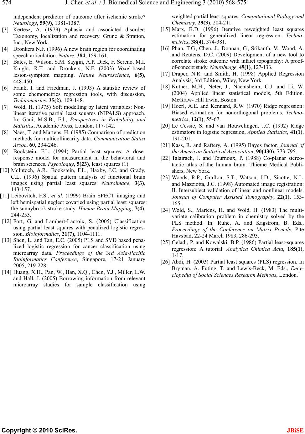

574 J. Chen et al. / J. Biomedical Science and Engineering 3 (2010) 568-575
independent predictor of outcome after ischemic stroke?
Neurology, 59(9), 1381-1387.
[3] Kertesz, A. (1979) Aphasia and associated disorder:
Taxonomy, localization and recovery. Grune & Stratton,
Inc., New York.
[4] Dronkers N.F. (1996) A new brain region for coordinating
speech articulation. Nature, 384, 159-161.
[5] Bates, E. Wilson, S.M. Saygin, A.P. Dick, F. Sereno, M.I.
Knight, R.T. and Dronkers, N.F. (2003) Voxel-based
lesion-symptom mapping. Nature Neuroscience, 6(5),
448-450.
[6] Frank, I. and Friedman, J. (1993) A statistic review of
some chemometrics regression tools, with discussion,
Technometrics, 35(2), 109-148.
[7] Wold, H. (1975) Soft modelling by latent variables: Non-
linear iterative partial least squares (NIPALS) approach.
In: Gani, M.S.B., Ed., Perspectives in Probability and
Statistics, Academic Press, London, 117-142.
[8] Naes, T. and Martens, H. (1985) Comparison of prediction
methods for multicollinearity data. Communication Statist
Assoc, 60, 234-246.
[9] Bookstein, F.L. (1994) Partial least squares: A dose-
response model for measurement in the behavioral and
brain sciences. Psycoloquy, 5(23), least squares (1).
[10] McIntoch, A.R., Bookstein, F.L., Haxby, J.C. and Grady,
C.L. (1996) Spatial pattern analysis of functional brain
images using partial least squares. Neuroimage, 3(3),
143-157.
[11] Leibovitch, F.S., et al. (1999) Brain SPECT imaging and
left hemispatial neglect covaried using partial least squares:
the sunnybrook stroke study. Human Brain Mapping, 7(4),
244-253.
[12] Fort, G. and Lambert-Lacroix, S. (2005) Classification
using partial least squares with penalized logistic regres-
sion. Bioinformatics, 21(7), 1104-1111.
[13] Shen, L. and Tan, E.C. (2005) PLS and SVD based pena-
lized logistic regression for cancer classification using
microarray data. Proceedings of the 3rd Asia-Pacific
Bioinformatics Conference, Singapore, 17-21 January
2005, 219-228.
[14] Huang, X.H., Pan, W., Han, X.Q., Chen, Y.J., Miller, L.W.
and Hall, J. (2005) Borrowing information from relevant
microarray studies for sample classification using
weighted partial least squares. Computational Biology and
Chemistry, 29(3), 204-211.
[15] Marx, B.D. (1996) Iterative reweighted least squares
estimation for generalized linear regression. Techno-
metrics, 38(4), 374-381.
[16] Phan, T.G., Chen, J., Donnan, G., Srikanth, V., Wood, A.
and Reutens, D.C. (2009) Development of a new tool to
correlate stroke outcome with infarct topography: A proof-
of-concept study. NeuroImage, 49(1), 127-133.
[17] Draper, N.R. and Smith, H. (1998) Applied Regression
Analysis, 3rd Edition, Wiley, New York.
[18] Kutner, M.H., Neter, J., Nachtsheim, C.J. and Li, W.
(2004) Applied linear statistical models, 5th Edition.
McGraw- Hill Irwin, Boston.
[19] Hoerl, A.E. and Kennard, R.W. (1970) Ridge regression:
Biased estimation for nonorthogonal problems. Techno-
metrics, 12(1), 55-67.
[20] Le Cessie, S. and van Houwelingen, J.C. (1992) Ridge
estimators in logistic regression, Applied Statistics, 41(1),
191-201.
[21] Kass, R. and Raftery, A. (1995) Bayes factor. Journal of
the American Statistical Association, 90(430), 773-795.
[22] Talairach, J. and Tournoux, P. (1988) Co-planar stereo-
tactic atlas of the human brain. Thieme Medical Publi-
shers, New York.
[23] Woods, R.P., Grafton, S.T., Watson, J.D., Sicotte, N.L.
and Mazziotta, J.C. (1998) Automated image registration:
II. Intersubject validation of linear and nonlinear models.
Journal of Computer Assisted Tomography, 22(1), 153-
165.
[24] Wold, S., Martens, H. and Wold, H. (1983) The multi-
variate calibration problem in chemistry solved by the
PLS method. In: Ruhe, A. and Kagstrom, B. Eds.,
Proceedings of the Conference on Matrix Pencils, Pite
Havsbad, 22-24 March 1983, 286-293.
[25] Geladi, P. and Kowalski, B.P. (1986) Partial least-squares
regression: A tutorial. Analytica Chimica Acta, 185(1),
1-17.
[26] Abdi, H. (2003) Partial least squares (PLS) regression. In
Bryman, A. Futing, T. and Lewis-Beck, M. Eds., Ency-
clopedia of Social Sciences Research Methods, London.

J. Chen et al. / J. Biomedical Science and Engineering 3 (2010) 568-575 575
APPENDIX
Maximum likelihood (ML) estimate of logistic regression
and Iterative reweighted least squares (IRLS)
When response variable y1, y2, …, yn are binary, taking
on the values 0 and 1 with probabilities and 1 – π, re-
spectively, with expect value E{y} = π, covariates xij{i =
1, 2, …, n; j = 1, 2,…, m} are also available, the logistic
regression model would construct by a canonical link
function
1
log 1
mT
jj
j
x





βx (A.1)
()
(
{}
1
T
T
a
a
e
E
e





βx
βx
y) (A.2)
where β = [β1, β2, …,βm], x =[x1, x2,…xm]. Thus the
probability distribution of y is
1
()(1)
y
fy 


y
(A.3)
Since the yi observations are independent, their joint
probability function is
1
12
11
(, ,...)()(1)
i
nn
i
y
y
niiii
ii
hy yyf y 



 (A.4)
It is often more convenient to work with the logarithm
of the joint probability function to find the maximum
likelihood estimate
1
12
1
11
log (,,...)log(1)
[ log()]log(1)
1
ii
n
y
y
ni
i
nn
i
ii
ii
i
hy yy
y











i
(A.5)
If we substitute (A.2) to (A.5) and consider equation
a1, we have
()
11
log(, )()log[1]
T
i
nn
T
ii
ii
Ly e






βx
ββx(A.6)
where xi is shorthand of [xi1, xi2, … xip] and L(α, β) re-
places h(y1, y2,…yn) to show explicitly that we now view
this function as the likelihood function of the parameters
to be estimated. Denote [1 ]
T
i
Zx
i
and [|]


γβ,
we have
1
()log ()[()log(1)]
i
n
ii
i
Ly e 

 
γZ
γγZ (A.7)
Taylor’s series tells us that an analytic function like
(A.7) can be approximated as
000 02
1
()( )()'( )() ''( )
2
 γγγγγγγ γ 
where γ0 is an estimated initial value of γ0. To maximize
()γ we can differentiate with respect to γ and solve for
γ
000
'( )'()() ''()0

 γγγγγ (A.9)
0
0
0
'( )
''( )
  γ γγ γ

 (A.10)
This suggests that we can start with an initial γ0 and
iteratively apply (A.10) until the algorithm reaches con-
vergence, at which point 0 ''( )0γand (A.10) does not
change. This is what called Newton optimization and in
the linear modeling setting is a vector. Newton’s method
has a generalization (Newton-Raphson) using the multi-
variate Taylor’s series.
20
001
()
[()]
T


 

γ
γγγγ
γγ

 (A.11)
where
2
()
T

 γ γγ
is the matrix of second derivates and
()

γ
γ
is the vector of first derivates.
The logistic log-likelihood for linear model becomes
1
()log(1 )
T
i
nT
ii
i
y


xγ
γxγe (A.12)
1
1
()(1)
()
TT
ii
nTT
ii i
i
yee



xγxγ
γxx
γ

1
1
(
1T
i
nT
i
i
y
e



xγx)
i
(A.13)
()
T

Xyπ
2
1
()(1)
nT
ii ii
T
i



 
 
γxx
γγ

T
XVX (A.14)
where V is a diagonal matrix with element W(i, i) equal
to (1 )
ii



. We can plug these results into (A.11)
01
()(
TT)

γγ XVXX yπ
101
()((
TT
XVXXVXγVyπ)) (A.15)
1
()
TT
XVXXVg
where 01 (
)

gXγVyπ. This process is called
iteratively reweighted least squares (IRLS).
0
(A.8)