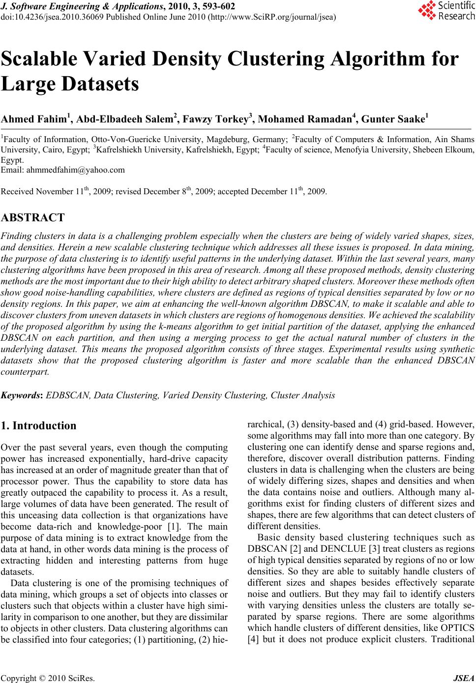J. Software Engineering & Applications, 2010, 3, 593-602
doi:10.4236/jsea.2010.36069 Published Online June 2010 (http://www.SciRP.org/journal/jsea)
Scalable Varied Density Clustering Algorithm for
Large Datasets
Ahmed Fahim1, Abd-Elbadeeh Salem2, Fawzy Torkey3, Mohamed Ramadan4, Gunter Saake1
1Faculty of Information, Otto-Von-Guericke University, Magdeburg, Germany; 2Faculty of Computers & Information, Ain Shams
University , Ca iro, Egypt; 3Kafrelshiekh University, Kafrelshiekh, Egypt; 4Faculty of science, Menofyia University, Shebeen Elkoum,
Egypt.
Received November 11th, 2009; revised December 8th, 2009; accepted December 11th, 2009.
ABSTRACT
Finding clusters in data is a challenging problem especially when the clusters are being of widely varied shapes, sizes,
and densities. Herein a n ew scalable clustering technique which addresses a ll these issues is proposed. In data mining,
the purpose of data clustering is to identify useful pa tterns in the underlying dataset. Within the last several yea rs, many
clustering alg orithms have been pr oposed in t his area of researc h. Among all these proposed methods, density clusterin g
methods are the most important due to their high ability to detect arbitrary shaped clusters. Moreover these methods often
show good noise-handling capabilities, where clusters are defined as regions of typical densities separated by low or no
density regions. In this paper, we aim at enhancing the well-known algorithm DBSCAN, to make it scalable and able to
discover clusters from uneven datasets in which clusters are regions of homogenous densities. We achieved the scalability
of the proposed algorithm by using the k-mea ns algorithm to get initial partitio n of the dataset, applying the enhanced
DBSCAN on each partition, and then using a merging process to get the actual natural number of clusters in the
underlying dataset. This means the proposed algorithm consists of three stages. Experimental results using synthetic
datasets show that the proposed clustering algorithm is faster and more scalable than the enhanced DBSCAN
counterpart.
Keywords: EDBSCAN, Data Clustering, Varied Density Clustering, Cluster Analysis
1. Introduction
Over the past several years, even though the computing
power has increased exponentially, hard-drive capacity
has increased at an order of magnitude greater than that of
processor power. Thus the capability to store data has
greatly outpaced the capability to process it. As a result,
large volumes of data have been generated. The result of
this unceasing data collection is that organizations have
become data-rich and knowledge-poor [1]. The main
purpose of data mining is to extract knowledge from the
data at hand, in other words data mining is the process of
extracting hidden and interesting patterns from huge
datasets.
Data clustering is one of the promising techniques of
data mining, which groups a set of objects into classes or
clusters such that objects within a cluster have high simi-
larity in comparison to one another, but they are dissimilar
to objects in other clusters. Data clustering algorithms can
be classified into four categories; (1) partitioning, (2) hie-
rarchical, (3) density-based and (4) grid-based. However,
some algorithms may fall into more than one category. By
clustering one can identify dense and sparse regions and,
therefore, discover overall distribution patterns. Finding
clusters in data is challenging when th e clusters are being
of widely differing sizes, shapes and densities and when
the data contains noise and outliers. Although many al-
gorithms exist for finding clusters of different sizes and
shapes, there are few al gorithms that can detect clusters of
different densities.
Basic density based clustering techniques such as
DBSCAN [2] and DENCLUE [3] treat clusters as regions
of high typical densities separated by regions of no or low
densities. So they are able to suitably handle clusters of
different sizes and shapes besides effectively separate
noise and outliers. But they may fail to identify clusters
with varying densities unless the clusters are totally se-
parated by sparse regions. There are some algorithms
which handle clu sters of different densities, like OPTICS
[4] but it does not produce explicit clusters. Traditional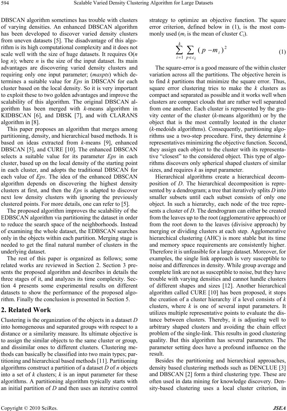

Scalable Varied Density Clustering Algorithm for Large Datasets 594
)
DBSCAN algorithm sometimes has trouble with clusters
of varying densities. An enhanced DBSCAN algorithm
has been developed to discover varied density clusters
from uneven datasets [5]. The disadvantage of this algo-
rithm is its high computational complexity and it does not
scale well with the size of huge datasets. It requires O(n
log n); where n is the size of the input dataset. Its main
advantages are discovering varied density clusters and
requiring only one input parameter; (ma xpts) which de-
termines a suitable value for Eps in DBSCAN for each
cluster based on the local density. So it is very important
to exploit these to two golden advantages and improve the
scalability of this algorithm. The original DBSCAN al-
gorithm has been merged with k-means algorithm in
KIDBSCAN [6], and DBSK [7], and with CLARANS
algorithm in [8].
This paper proposes an algorithm that merges among
partitioning, de nsity, a nd h iera r chical ba sed m etho ds. It is
based on ideas extracted from k-means [9], enhanced
DBSCAN [5], and CURE [10]. The enhanced DBSCAN
selects a suitable value for its parameter Eps in each
cluster, based up on the local density of the starting point
in each cluster, and adopts the traditional DBSCAN for
each value of Eps. The idea of the enhanced DBSCAN
algorithm depends on discovering the highest density
clusters at first, and then the Eps is adapted to discover
next low density clusters with ignoring the previously
clustered points. For more details, one can refer to [5].
The proposed algorithm improves the scalability of the
EDBSCAN algorithm via partitioning the dataset in order
to reduce the search space of the neighborhoods. Instead
of examining the whole dataset, the EDBSCAN searches
only in the objects within each partition. Merging stag e is
needed to get the final natural number of clusters in the
underlying dat a se t .
The rest of this paper is organized as follows; some
related works are reviewed in Section 2. Section 3 pre-
sents the proposed algorithm and describes in details the
three stages of it, and analyzes its time complexity. Sec-
tion 4 presents some experimental results on different
datasets to show the performance of the proposed algo-
rithm. Finally the conclusion is presented in Section 5.
2. Related Work
Clustering is the organization of the objects in a dataset D
into homogeneous and separated groups with respect to a
distance or a similarity measure. Its ultimate objective is
to assign the similar objects to the same cluster or group,
and dissimilar ones to different clusters. Clustering me-
thods can basically be classified into two main types; par-
titioning and hierarchical base d methods [11]. Partitioning
algorithms construct a partition of a dataset D of n objects
into a set of k clusters; k is an input parameter for these
algorithms. A partitioning algorithm typically starts with
an initial partition of D and then uses an iterative control
strategy to optimize an objective function. The square
error criterion, defined below in (1), is the most com-
monly used (mi is the mean of cluster Ci).
2
1(
k
i
ipc
i
p
m


 (1)
The square -error is a good m easure of the within cluster
variation across all the partiti ons. The objective herein is
to find k partitions that minimize the square error. Thus,
square error clustering tries to make the k clusters as
compact and se parated as possibl e and it wo rks well whe n
clusters are compact clouds that are rather well separated
from one another. Each cluster is represented by the gra-
vity center of the cluster (k-means algorithm) or by the
object that is the most centrally located in the cluster
(k-medoids algorithms). Consequently, partitioning algo-
rithms use a two-step procedure. First, they determine k
representatives minimizing the objective function. Second,
they assign each object to the cluster with its representa-
tive “closest” to the considered object. This type of algo-
rithms discovers only spherical shaped clusters of similar
sizes, and requires k as input parameter.
Hierarchical algorithms create a hierarchical decom-
position of D. The hierarchical decomposition is repre-
sented by a dendrogram; a tree that iteratively splits D into
smaller subsets until each subset consists of only one
object. In such a hierarchy, each node of the tree repre-
sents a cluster of D. The dendrogram can either be c reated
from the leaves up to the root (agglom erative approach ) or
from the root down to the leaves (divisive approach) by
merging or dividing clusters at each step. Agglomerative
hierarchical clustering (AHC) is more stable but its time
and memory space requirements are consistently higher.
Therefore it is unfeasible for a large dataset. Moreover, for
examples, the single link approach is very susceptible to
noise and di fferences in de nsit y. While grou p avera ge and
complete link are not as susceptible to noise, but they have
trouble with varying densities and cannot hand le clusters
of different shapes and sizes [12]. Another hierarchical
algorithm called CURE [10] has been proposed, it stops
the creation of a cluster hierarchy if a level consists of k
clusters, where k is one of several input parameters. It
utilizes multiple represen tative points to evaluate the dis-
tance between clusters. Thereby, it is adjusting well to
arbitrary shaped clusters and avoiding the chain effect
problem of th e sin g le-link. Th is results in go od clu stering
quality. But this algorithm has several parameters. The
parameter setting does have a profound influence on the
result.
Besides the partitioning and hierarchical approaches,
density based clustering methods such as DENCLUE [3]
and DBSCAN [2] for m a third clustering type. These are
often used in data mining for knowledge discovery. Den-
sity-based clustering uses a local cluster criterion, in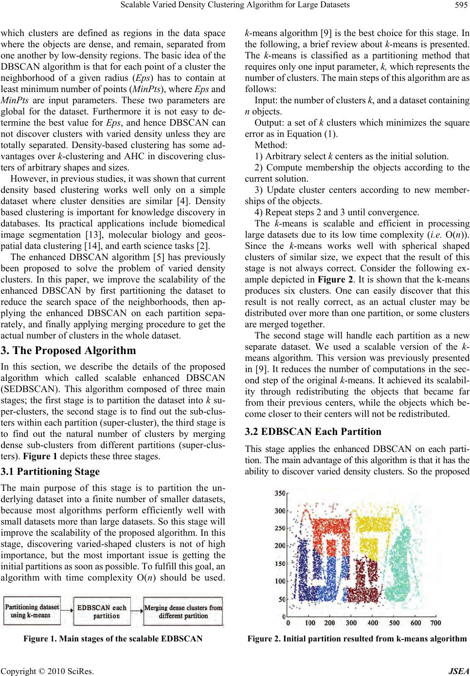

Scalable Varied Density Clustering Algorithm for Large Datasets595
which clusters are defined as regions in the data space
where the objects are dense, and remain, separated from
one another by low-density regions. The basic idea of the
DBSCAN algorithm is that for each point of a cluster the
neighborhood of a given radius (Eps) has to contain at
least minimum number of points (MinPts), where Eps and
MinPts are input parameters. These two parameters are
global for the dataset. Furthermore it is not easy to de-
termine the best value for Eps, and hence DBSCAN can
not discover clusters with varied density unless they are
totally separated. Density-based clustering has some ad-
vantages over k-clustering and AHC in discovering clus-
ters of ar bitrary shapes and sizes.
However, in previous studies, it was shown that current
density based clustering works well only on a simple
dataset where cluster densities are similar [4]. Density
based clustering is important for knowledge discovery in
databases. Its practical applications include biomedical
image segmentation [13], molecular biology and geos-
patial data clustering [14], and earth science tasks [2].
The enhanced DBSCAN algorithm [5] has previously
been proposed to solve the problem of varied density
clusters. In this paper, we improve the scalability of the
enhanced DBSCAN by first partitioning the dataset to
reduce the search space of the neighborhoods, then ap-
plying the enhanced DBSCAN on each partition sepa-
rately, and finally applying merging procedure to get the
actual number of clusters in the whole dataset.
3. The Proposed Algorithm
In this section, we describe the details of the proposed
algorithm which called scalable enhanced DBSCAN
(SEDBSCAN). This algorithm composed of three main
stages; the first stage is to partition the dataset into k su-
per-clusters, the second stage is to find out the sub-clus-
ters within each partition (super-cluster), the third stage is
to find out the natural number of clusters by merging
dense sub-clusters from different partitions (super-clus-
ters). Figure 1 depicts these three stages.
3.1 Partitioning Stage
The main purpose of this stage is to partition the un-
derlying dataset into a finite number of smaller datasets,
because most algorithms perform efficiently well with
small datasets more than large datasets. So this stage will
improve the scalability of th e proposed algorithm. In this
stage, discovering varied-shaped clusters is not of high
importance, but the most important issue is getting the
initial partitions as soon as possible. To fulfill this goal, an
algorithm with time complexity O(n) should be used.
Figure 1. Main stages of the scalable EDBSCAN
k-means algorithm [9] is the best choice for th is stage. In
the following, a brief rev iew about k-means is presented.
The k-means is classified as a partitioning method that
requires only one input parameter, k, which represents the
number of clusters. T he main s teps of this algor ithm are as
follows:
Input: the number of clusters k, and a dat aset contai ning
n objects.
Output: a set of k clusters which minimizes the square
error as in Equation (1).
Method:
1) Arbitrary select k centers as the initial solution.
2) Compute membership the objects according to the
current solution.
3) Update cluster centers according to new member-
ships of the objects.
4) Repeat steps 2 and 3 until converg en ce.
The k-means is scalable and efficient in processing
large datasets due to its low time complexity (i.e. O(n)).
Since the k-means works well with spherical shaped
clusters of similar size, we expect that the result of this
stage is not always correct. Consider the following ex-
ample depicted in Figure 2. It is shown that the k-means
produces six clusters. One can easily discover that this
result is not really correct, as an actual cluster may be
distributed over more than one partition, or some clusters
are merged together.
The second stage will handle each partition as a new
separate dataset. We used a scalable version of the k-
means algorithm. This version was previously presented
in [9]. It reduces the number of computations in the sec-
ond step of the original k-means. It achieved its scalabil-
ity through redistributing the objects that became far
from their previous centers, while the objects which be-
come closer to their centers will not be redistributed.
3.2 EDBSCAN Each Partition
This stage applies the enhanced DBSCAN on each parti-
tion. The main advantage of this algorithm is that it has the
ability to discover varied density clusters. So the proposed
Figure 2. Initial partition resulted from k-means algorithm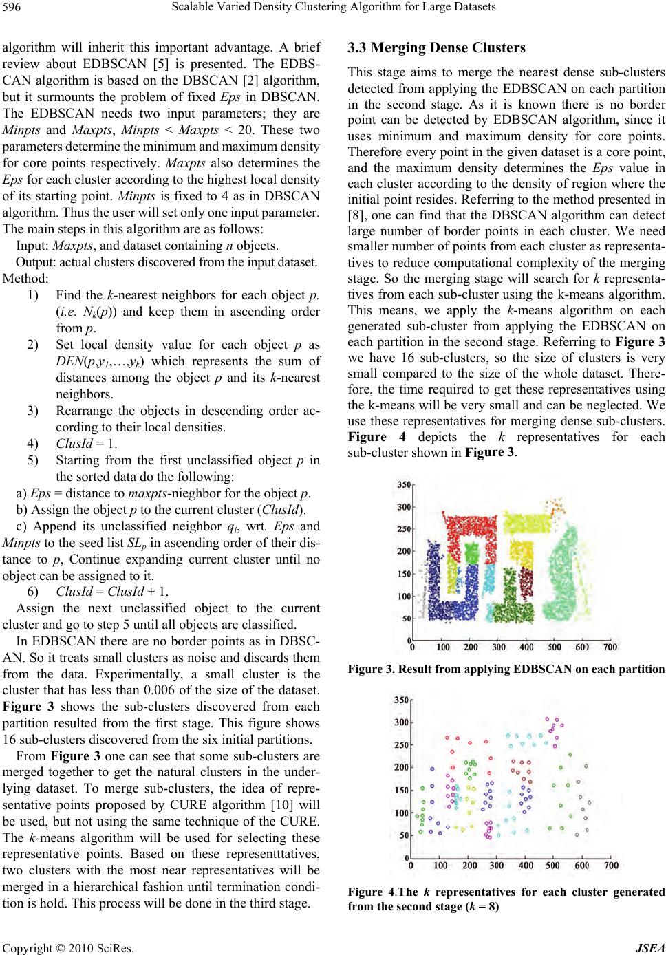

Scalable Varied Density Clustering Algorithm for Large Datasets 596
ure 3.
algorithm will inherit this important advantage. A brief
review about EDBSCAN [5] is presented. The EDBS-
CAN algorithm is based on the DBSCAN [2] algorithm,
but it surmounts the problem of fixed Eps in DBSCAN.
The EDBSCAN needs two input parameters; they are
Minpts and Maxpts, Minpts < Maxpts < 20. These two
parameters det ermine the minim um and maximum densi ty
for core points respectively. Maxpts also determines the
Eps for each cluster according to the highest local density
of its starting point. Minpts is fixed to 4 as in DBSCAN
algorithm. Thus the user will set only one input parameter.
The main steps in this algorithm are as follows:
Input: Maxpts, and dataset containing n obj ects.
Output: actual clusters discovered from t he input dataset.
Method:
1) Find the k-nearest neighbors for each object p.
(i.e. Nk(p)) and keep them in ascending order
from p.
2) Set local density value for each object p as
DEN(p,y1,…,yk) which represents the sum of
distances among the object p and its k-nearest
neighbors.
3) Rearrange the objects in descending order ac-
cording to their local densities.
4) ClusId = 1.
5) Starting from the first unclassified object p in
the sorted data do the following:
a) Eps = distance to maxpts-nieghbor for the object p.
b) Assign the object p to the current cluster (ClusId).
c) Append its unclassified neighbor qi, wrt. Eps and
Minpts to the seed list SLp in ascending order of their dis-
tance to p, Continue expanding current cluster until no
object can be assigned to it.
6) ClusId = ClusId + 1.
Assign the next unclassified object to the current
cluster and go to step 5 until all objects are classified.
In EDBSCAN there are no border points as in DBSC-
AN. So it treats small clusters as noise and discards them
from the data. Experimentally, a small cluster is the
cluster that has less than 0.006 of the size of the dataset.
Figure 3 shows the sub-clusters discovered from each
partition resulted from the first stage. This figure shows
16 sub-clusters discovered from the six initial partitions.
From Figure 3 one can see that some sub-clusters are
merged together to get the natural clusters in the under-
lying dataset. To merge sub-clusters, the idea of repre-
sentative points proposed by CURE algorithm [10] will
be used, but not using the same technique of the CURE.
The k-means algorithm will be used for selecting these
representative points. Based on these representttatives,
two clusters with the most near representatives will be
merged in a hierarchical fashion until termination condi-
tion is hold. This process will be don e in the third stage.
3.3 Merging Dense Clusters
This stage aims to merge the nearest dense sub-clusters
detected from applying the EDBSCAN on each partition
in the second stage. As it is known there is no border
point can be detected by EDBSCAN algorithm, since it
uses minimum and maximum density for core points.
Therefore every point in the given dataset is a core point,
and the maximum density determines the Eps value in
each cluster according to the density of region where the
initial point resides. Referring to the method presented in
[8], one can find that the DBSCAN algorithm can detect
large number of border points in each cluster. We need
smaller number of points from each cluster as representa-
tives to reduce computational complexity of the merging
stage. So the merging stage will search for k representa-
tives from each sub-cluster using the k-means algorithm.
This means, we apply the k-means algorithm on each
generated sub-cluster from applying the EDBSCAN on
each partition in the second stage. Referring to Figure 3
we have 16 sub-clusters, so the size of clusters is very
small compared to the size of the whole dataset. There-
fore, the time required to get these representatives using
the k-means will be very small and can be neglected. We
use these representatives for merging dense sub-clusters.
Figure 4 depicts the k representatives for each
sub-cluster shown in Fig
Figure 3. Result from applying EDBSCAN on each partition
Figure 4.The k representatives for each cluster generated
from the second stage (k = 8)

Scalable Varied Density Clustering Algorithm for Large Datasets597
Two dense sub-clusters with the most nearest repre-
sentatives will be merged together in a hierarchical form.
This idea is similar to that was propo sed by CURE algo-
rithm [10]. We need a threshold to stop the merging
process. This may be a simple problem because we al-
ready have some information about the data from the
previous stages; like the number of sub-clusters, Eps in
each cluster (density level of each cluster), distances
among cluster’s representatives. Intuitively, two sub-
clusters in second stage are not allowed to be merged
together if they are belonging to the same partitio n (sup er
cluster) in the first stage.
The algorithm arranges the merging distances in as-
cending order. By examining the plot of distances, we
can easily select threshold distance to stop the merging
process. Figure 5 presents the merging distances plot for
the sub-clusters in Figure 3.
Since we have 16 sub-clusters from the second stage,
we need 15 merging steps for merging all sub-clusters
into a single cluster. We search for the gaps in distances
plot. From Figure 5 we notice that only one gap between
distances 28.7 and 47.6. So any value between these two
values will be a threshold distance. The merging process
is applied seven times so that the final number of clusters
will be 16-7 = 9 clusters as shown in Figure 6.
We can get rid of the smallest three clusters as noise,
and return the remaining six clusters as a final result.
3.4 Complexity Analysis
The execution time of the proposed algorithm is com-
posed of three components; the first one is the time for
executing the k-means algorithm on the entire dataset
which is O(n), where n is the size of the input dataset.
The second component is the time for executing the
EDBSCAN algorithm on each part resulting from the k-
means in the first stage, the EDBSCAN requires O(m2) if
it doesn’t use an index structure like R*-tree, or O(m log
m) if it uses R*-tree; where m is the size of the input
dataset, and m is very smaller than n since m is the size
of one part of the original dataset. The third component is
the time for getting the k representatives from each sub-
cluster, and the merging process, this time is very small
and can be neglected, because we apply the k-means al-
gorithm on each sub-cluster which is very small com-
pared with the size of the original dataset, and the total
number of representatives is also very small compared to
the original dataset size. Furthermore, we don’t find the
distances among representatives belonging to the same
part in the initial partition. Hence the entire execution
time of the proposed algorithm is O(n + m log m) which
is definitely smaller than O(n log n).
4. Experimental Results
In this section the performance of the proposed algorithm
is evaluated. This algorithm has been implemente d in C++.
Figure 5. Merging distances plot
Figure 6. Natural number of clusters in dataset
We have used m any synthetic data sets to test the pr oposed
algorithm. The experiments have been done on seven
different datasets containing 2D points. The first dataset
has six clusters of different sizes, shapes, and orientation,
as well as random noise points and special artifacts such
as streaks running across clust ers, this dataset is used as an
example in Figure 2. The second dataset has six clusters
of different shapes. Moreover, it also contains random
noise and special artifacts, such as a collection of points
forming horizontal streak, this dataset is shown in Figure
7. The third dataset has eight clusters of different shapes,
sizes, and orientation, some of which are inside the space
enclosed by other clusters. Moreover, it also contains
random noise and special artifacts, such as a collection of
points forming vertical streaks. This dataset is shown in
Figure 8. The fourt h dataset h as eight clust ers of differe nt
shapes, sizes, densities, and orientation, as well as random
noise. A particularly challenging feature of this data set is
that the clust ers are very c lose to each othe r and the y ha ve
different densities, this dataset is shown in Figure 9. The
fifth dataset has four clusters of different shape, size, and
density. A particularly challenging feature of this data set
is that, the clusters are very close to each other and they
have different densities, this dataset is shown in Figure 10.
The sixth and seventh datasets have clusters of different

Scalable Varied Density Clustering Algorithm for Large Datasets 598
Figure 7. Clusters obtained from dataset 2
sizes and densities. These datasets are shown in Figures
11 and 12. The last three datasets are presented here to
insure that the proposed algorithm is very efficient in
discovering varied density clusters without requiring se-
parating regions with low density.
We evaluate t he performance of the propose d algorithm
compared to the original EDBSCAN using different
synthetic datasets include noise; the sizes of these datasets
are ranging from 3147 to 10000 points in two-dimensions
Figure 8. Clusters obtained from dataset 3
(2D), and they contain varied shaped, size, and density
clusters. Figure 7 shows the three steps of the proposed
algorithm on dataset 2 of size 8000 points.
For comparing the proposed algorithm with the original
EDBSCAN, the same value for the parameter maxpts in
both EDBSCAN and the proposed algorithm is used in
order to demonstrate the higher enhancement of the pro-
posed algorithm. Figure 8 shows the three steps of the
proposed algorith m on the third dataset con taining 10000
points.

Scalable Varied Density Clustering Algorithm for Large Datasets599
Figure 9. Clusters obtained from dataset 4
However data set 3 has cl usters of va ried sha pes that are
nested with each other, the proposed algorithm could
discover the right clusters in the data. There is a small
mistake in the ring cluster that has two different spherical
clusters within it. This cluster has three levels of density in
Figure 10. Clusters obtained from dataset 5
its right half. This mistake resulted from the EDBSCAN
which considered the small cluster as outlier and removed
it from the data, but this problem can easily be resolved by
assigning the outlier clusters to the nearest cluster. Figure
9 shows the three steps of the proposed algorithm on

Scalable Varied Density Clustering Algorithm for Large Datasets 600
Figure 11. Clusters obtained from dataset 6
dataset 4 of size 8000 poin ts.
Dataset 5 has four clusters of varied shapes, sizes and
densities. The proposed algorithm could successfully
discover the correct clusters. Figure 10 shows the result
on dataset 5 that has varied-density clusters with no sepa-
ration among them.
Figure 12. Clusters obtained from dataset 7
From Figures 11 and 12, one can find that the final
result is the same as the result from EDBSCAN in step 2
of the proposed algorithm. This is because the clusters in
the same part are not allowed to be merged, and each part
has clusters that are totally separated from clusters in other
parts.

Scalable Varied Density Clustering Algorithm for Large Datasets601
From the experimental result, we can deduce that the
proposed algorithm is able to discover clusters with varied
shapes, sizes, and densities efficiently. It can easily be
noticed that the result obtained by the proposed algori t hm
is not exactly similar to the one of EDBSCAN on the
entire dataset. Instead, the proposed algorithm produces
additional small clusters that are discarded as noise by
EDBSCAN on the entire dataset. This is not an irresolv-
able problem. If we want to get the identical result of
EDBSCAN, we should remove the small clusters as noise.
The results of the original EDBSCAN on the entire data-
sets are shown in Figure 13.
Figure 13. The results from the original EDBSCAN on the
entire datasets
The proposed algorithm is more scalable than EDBS-
CAN algorithm, the scalability of the proposed algorith m
comes from partitioning the orig inal dataset into finite set
of smaller datasets in the first stage, and depending on k
representatives from each sub-cluster to get the actual
clusters in the original dataset. The following Figure 14
depicts the execution time of the proposed algorithm and
EDBSCAN without using an index structure like R*-tree
or canopies. We use only the fist four datasets because
the other datasets are very small. From Figure 14 it is
noticed that the proposed algorithm (SEDBSCAN) rea-
ches a speed up factor 5.25, 5, 5.33, an d 5.25 for datasets
1, 2, 3, and 4 respectively.
5. Conclusions
This paper has introduced a scalable and efficient clus-
tering algorithm for discovering clusters with varied
shapes, sizes, and densities. The proposed algorithm has
exploited all the advantages of previous different algo-
rithms (e.g., the scalability of the k-means, and the ability
of discovering clusters from uneven datasets of the
EDBSCAN, and the idea of multiple representatives taken
from the CURE algorithm, and finally the idea of local
density taken from the DENCLUE Algorithm) and has
overcame their disadvantages. So this algorithm collects
ideas from partitioning, hierarchical, and density based
methods. Generally speaking, combining all these ideas
into the proposed algorithm allows it to be scalable and
more efficient in discovering clusters of varied density.
The experimental results have given a clear indication on
the scalability of the proposed algorithm. Furthermore the
proposed algorithm has better performance than EDBSC-
AN with speed up factor up to 5 times. Additionally, the
algorithm can be partially imp lemented in parallel (in the
second stage) which help s in improv ing th e scalab ility b y
a significant factor.
Figure 14. The execution time comparison

Scalable Varied Density Clustering Algorithm for Large Datasets 602
REFERENCES
[1] J. MacLennan, Z. Tang and B. Crivat, “Data Mining with
SQL Server 2008,” Wiley Publishing, Indiana, 2009.
[2] M. Ester, H. P. Kriegel, J. Sander and X. Xu, “A Density
Based Algorithm for Discovering Clusters in large Spatial
Datasets with Noise,” Proceedings of International
Conference on Knowledge Discovery and Data Mining,
1996, pp. 226-231.
[3] A. Hinneburg and D. Keim, “An Efficient Approach to
Clustering in Large Multimedia databases with Noise,”
Proceedings Int ernational Conf e r e n ce on Knowled g e Di s -
covery and Data Mining, 1998, pp. 58-65.
[4] M. Ankerst, M. Breunig, H. P. Kriegel and J. Sandler,
“OPTICS: Ordering Points to Identify the Clustering
Structure,” Proceedings of the International Conference
on Management of Data (SIGMOD’99), 1999, pp. 49-60.
[5] A. Fahim, G. Saake, A. Salem, F. Torkey and M. Rama-
dan, “Enhanced Density Based Spatial clustering of
Application with Noise,” in Proceedings of the 2009 Inter-
national Conference on Data Mining, Las Vegas, July
2009, pp. 517-523.
[6] C.-F. Tsai and C.-W. Liu, “KIDBSCAN: A New Efficient
Data Clustering Algorithm,” Artificial Intelligence and
Soft Computing-ICAISC, Springer, Berlin/Heidelberg,
2006, pp. 702-711.
[7] R. Xin and C. H. Duo, “An Improved Clustering Algo-
rithm,” International Symposium on Computatio na l Intel l-
igence and Design, 2008, pp. 394-397.
[8] Y. El-Sonbaty, M. Ismail and M. Farouk, “An Efficient
Density Based Clustering Algorithm for Large Data-
bases,” Proceedings of the 16th IEEE International
Conference on Tools with Artificial Intelligence (ICTAI),
2004, pp. 673-677.
[9] A. Fahim, A. Salem, F. Torkey and M. Ramadan, “An
Efficient Enhanced k-Means Clustering Algorithm,”
Journal of Zhejiang University Science A, Vol. 7, No. 10,
2006, pp. 1626-1633.
[10] S. Guha, R. Rastogi and K. Shim, “CURE: An Efficient
Clustering Algorithms for Large Databases,” Procee-
dings of ACM SIGMOD International Conference on
Management of Data, Seattle, 1998, pp. 73-84.
[11] A. K. Jain, M. N. Murty and P. J. Flynn, “Data Clustering:
A Review,” ACM Computing Surveys, Vol. 31, No. 3,
September 1999, pp. 264-323.
[12] L. Ertoz, M. Steinbach and V. Kumar, “A New Shared
Nearest Neighbor Clustering Algorithm and its Appli-
cations,” Worksho p on C lu steri ng High Dime nsion a l Data
and its Applications at 2nd SIAM International Con-
ference on Data Mining, 2002.
[13] M. Emre Celebi, Y. Alp Aslandogan and P. R. Bergs-
tresser, “Mining Biomedical Images with Density-Based
Clustering,” Proceedings of the International Confer-
ence on Information Technology: Coding and Computing,
Washington, DC, IEEE Computer Society, Vol. 1, 2005,
pp. 163-168.
[14] J. Sander, M. Ester, H.-P. Kriegel and X. Xu “Density-
Based Clustering in Spatial Databases: The Algorithm
GDBSCAN and its Applications,” Data Mining and
Knowledge Discovery, Vol. 2, No. 2, 1998, pp. 169-194.