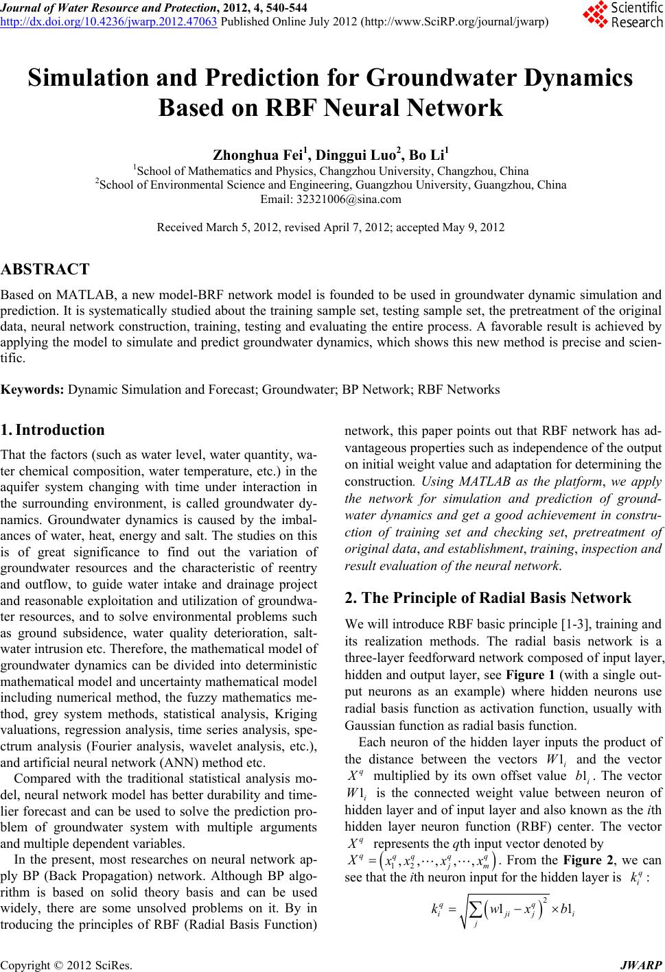Journal of Water Resource and Protection, 2012, 4, 540-544
http://dx.doi.org/10.4236/jwarp.2012.47063 Published Online July 2012 (http://www.SciRP.org/journal/jwarp)
Simulation and Prediction for Groundwater Dynamics
Based on RBF Neural Network
Zhonghua Fei1, Dinggui Luo2, Bo Li1
1School of Mathematics and Physics, Changzhou University, Changzhou, China
2School of Environmental Science and Engineering, Guangzhou University, Guangzhou, China
Received March 5, 2012, revised April 7, 2012; accepted May 9, 2012
ABSTRACT
Based on MATLAB, a new model-BRF network model is founded to be used in groundwater dynamic simulation and
prediction. It is systematicall y studied about the training samp le set, testing sample set, the pretreatment of the original
data, neural network construction, training, testing and evaluating the entire process. A favorable result is achieved by
applying the model to simulate and predict groundwater dynamics, which shows this new method is precise and scien-
tific.
Keywords: Dynamic Simulation and Forecast; Groundwater; BP Network; RBF Networks
1. Introduction
That the factors (such as water level, water quantity, wa-
ter chemical composition, water temperature, etc.) in the
aquifer system changing with time under interaction in
the surrounding environment, is called groundwater dy-
namics. Groundwater dynamics is caused by the imbal-
ances of water, heat, energy and salt. The studies on this
is of great significance to find out the variation of
groundwater resources and the characteristic of reentry
and outflow, to guide water intake and drainage project
and reasonable exploitation and utilization of groundwa-
ter resources, and to solve environmental problems such
as ground subsidence, water quality deterioration, salt-
water intrusion etc. Therefore, the mathematical model of
groundwater dynamics can be divided into deterministic
mathematical model and uncertainty mathematical mode l
including numerical method, the fuzzy mathematics me-
thod, grey system methods, statistical analysis, Kriging
valuations, regression analysis, time series analysis, spe-
ctrum analysis (Fourier analysis, wavelet analysis, etc.),
and artificial neural network (ANN) method etc.
Compared with the traditional statistical analysis mo-
del, neural network model has better durability and time-
lier forecast and can be used to solve the prediction pro-
blem of groundwater system with multiple arguments
and multiple depend ent variables.
In the present, most researches on neural network ap-
ply BP (Back Propagation) network. Although BP algo-
rithm is based on solid theory basis and can be used
widely, there are some unsolved problems on it. By in
troducing the principles of RBF (Radial Basis Function)
network, this paper points out that RBF network has ad-
vantageous properties such as independence of the output
on initial weight value and adaptatio n fo r determining the
construction. Using MATLAB as the platform, we apply
the network for simulation and prediction of ground-
water dynamics and get a good achievement in constru-
ction of training set and checking set, pretreatment of
original da ta, and establishment, training, inspection and
result evaluation of the neural network.
2. The Principle of Radial Basis Network
We will introduce RBF basic principle [1-3], train ing and
its realization methods. The radial basis network is a
three-layer feedforward network composed of input layer,
hidden and output layer, see Figure 1 (with a single out-
put neurons as an example) where hidden neurons use
radial basis function as activation function, usually with
Gaussian function as radial basis function.
Each neuron of the hidden layer inputs the product of
the distance between the vectors i W and the vector 1
q
X
multiplied by its own offset value i. The vector
i is the connected weight value between neuron of
hidden layer and of input layer and also known as th e ith
hidden layer neuron function (RBF) center. The vector
1b
1W
q
X
represents the qth input vector denoted by


,,,,,
qqq q q
12
j
m
X
x
xxx 
q
i
k

. From the Figure 2, we can
see that the ith neuron input for the hidden layer is :
21
1
qq
ii ji j
j
kb wx  


C
opyright © 2012 SciRes. JWARP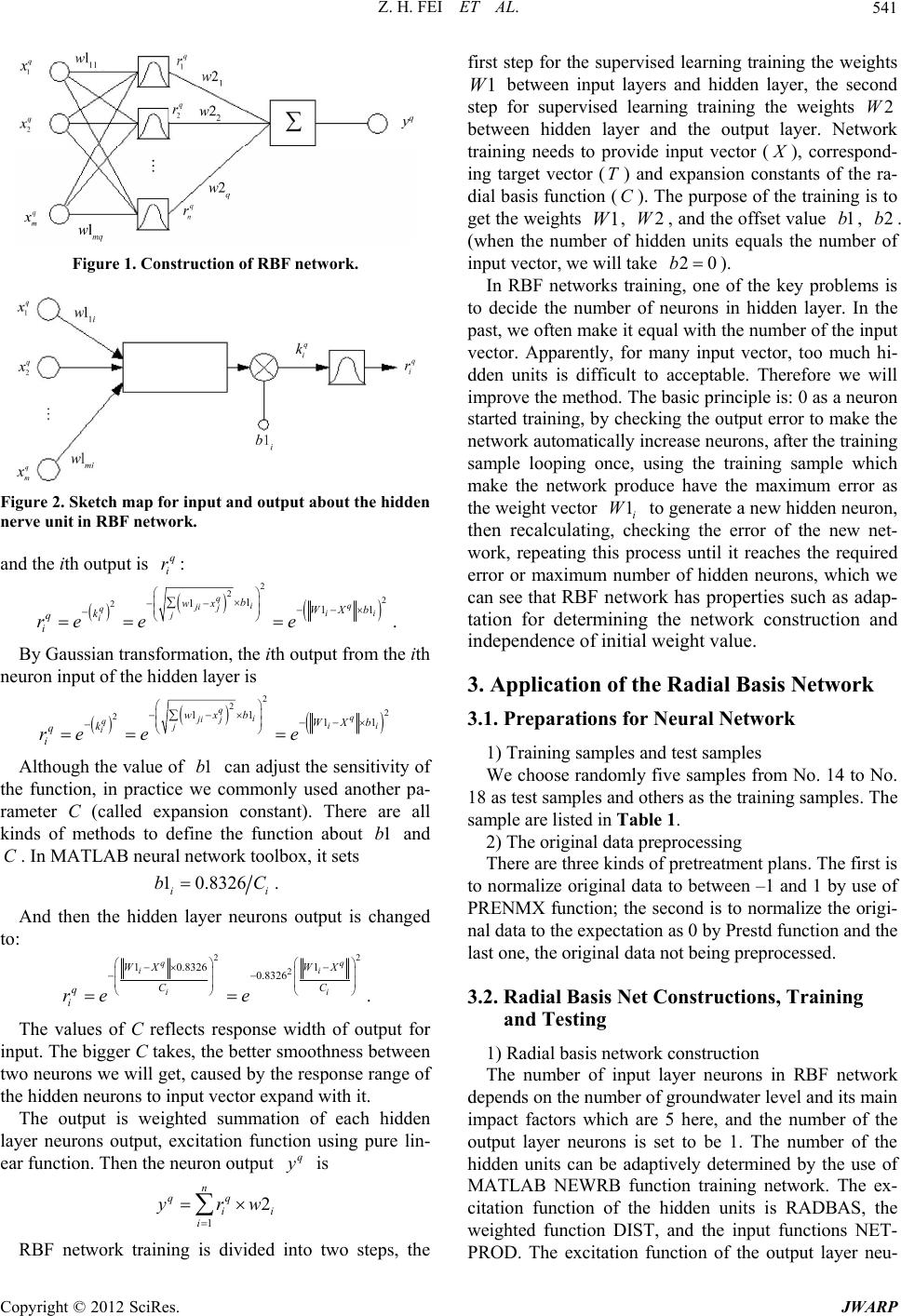

Z. H. FEI ET AL. 541
Figure 1. Construction of RBF network.
Figure 2. Sketch map for input and output abo ut the hidde n
nerve unit in RBF networ k.
and the ith output is :
q
i
r



2
11
q
ii
WXb
e



2
2
21
1qi
ji j
qj
i
b
wx
k
q
i
re e







 .
By Gaussian transformation, the ith output from the ith
neuron input of the hidden layer is



2
11
q
ii
WXb
e
 

1b
1b
C
2
2
21
1qi
ji j
qj
i
b
wx
k
q
i
re e







Although the valu e of can adjust the sensitivity of
the function, in practice we commonly used another pa-
rameter C (called expansion constant). There are all
kinds of methods to define the function about and
. In MATLAB neural network toolbox, it sets
10.8326
ii
bC.
And then the hidden layer neurons output is changed
to:
22
21
0.8326 q
ii
i
WX
C





q
1 0.8326
q
i
WX
C q
i
re e






.
The values of C reflects response width of output for
input. The bigger C takes, the better smoothness between
two neurons we will g et, caused by th e response range o f
the hidden neurons to input vector expand with it.
The output is weighted summation of each hidden
layer neurons output, excitation function using pure lin-
ear function. Then the neuron output
y
is
1
2
qq
ii
i
yrw



1W2
n
RBF network training is divided into two steps, the
first step for the supervised learning training the weights
between input layers and hidden layer, the second
step for supervised learning training the weights W
between hidden layer and the output layer. Network
training needs to provide input vector (
X
), correspond-
ing target vector (T) and expansion constants of the ra-
dial basis function (C). The purpose of the training is to
get the weights , , and the offset value , .
(when the number of hidden units equals the number of
input vector, we will take ).
1W2W1b2b
20b
1W
In RBF networks training, one of the key problems is
to decide the number of neurons in hidden layer. In the
past, we often make it equal with the number of the input
vector. Apparently, for many input vector, too much hi-
dden units is difficult to acceptable. Therefore we will
improve the method. The basic pr incip le is: 0 as a neuron
started traini ng, by checking the ou tput error to make the
network automatically increase neurons, after the training
sample looping once, using the training sample which
make the network produce have the maximum error as
the weight vector i to generate a new hidden neuron,
then recalculating, checking the error of the new net-
work, repeating this process until it reaches the required
error or maximum number of hidden neurons, which we
can see that RBF network has properties such as adap-
tation for determining the network construction and
independence of initial weight value.
3. Application of the Radial Basis Network
3.1. Preparations for Neural Network
1) Training samples and test samples
We choose randomly five samples from No. 14 to No.
18 as test samples and others as the training samples. The
sample are listed in Table 1.
2) The original data preprocessing
There are three kinds of pretreatment plans. The first is
to normalize original data to between –1 and 1 by use of
PRENMX function; the second is to normalize the origi-
nal data to the expectation as 0 by Prestd function and the
last one, the original data not being preprocessed.
3.2. Radial Basis Net Constructions, Training
and Testing
1) Radial basis network construction
The number of input layer neurons in RBF network
depends on the number of groundwater level and its main
impact factors which are 5 here, and the number of the
output layer neurons is set to be 1. The number of the
hidden units can be adaptively determined by the use of
MATLAB NEWRB function training network. The ex-
citation function of the hidden units is RADBAS, the
weighted function DIST, and the input functions NET-
PROD. The excitation function of the output layer neu-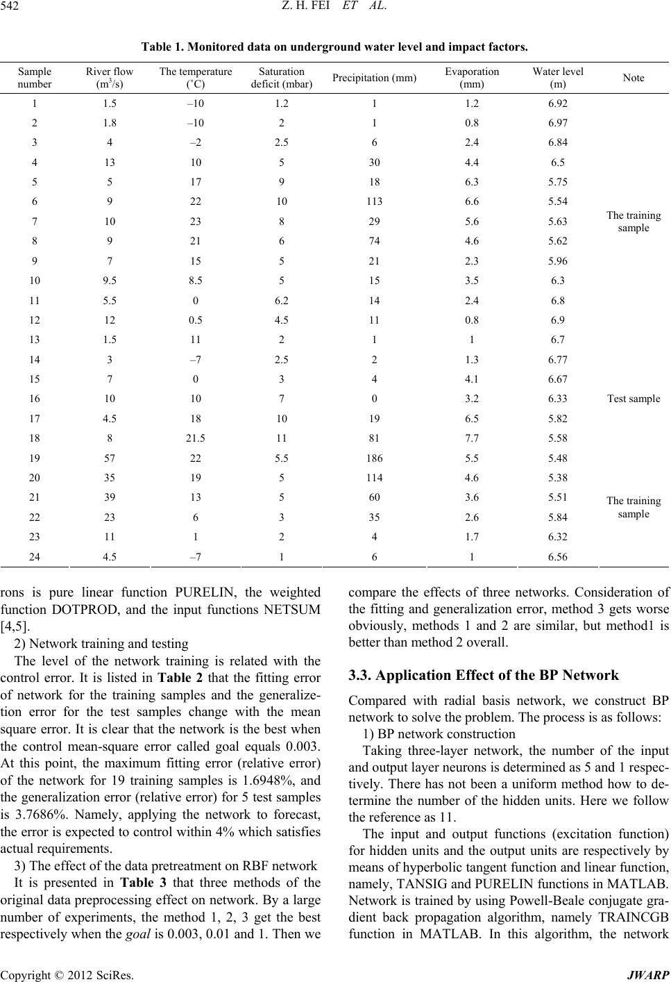

Z. H. FEI ET AL. 542
Table 1. Monitored data on undergr ound water level and impact factor s.
Sample
number River flow (m3/s) The temperature (˚C) Saturation deficit (mba r)Precipitation (mm)Evaporation (mm) Water level (m) Note
1 1.5 –10 1.2 1 1.2 6.92
2 1.8 –10 2 1 0.8 6.97
3 4 –2 2.5 6 2.4 6.84
4 13 10 5 30 4.4 6.5
5 5 17 9 18 6.3 5.75
6 9 22 10 113 6.6 5.54
7 10 23 8 29 5.6 5.63
8 9 21 6 74 4.6 5.62
9 7 15 5 21 2.3 5.96
10 9.5 8.5 5 15 3.5 6.3
11 5.5 0 6.2 14 2.4 6.8
12 12 0.5 4.5 11 0.8 6.9
13 1.5 11 2 1 1 6.7
The training
sample
14 3 –7 2.5 2 1.3 6.77
15 7 0 3 4 4.1 6.67
16 10 10 7 0 3.2 6.33
17 4.5 18 10 19 6.5 5.82
18 8 21.5 11 81 7.7 5.58
Test sample
19 57 22 5.5 186 5.5 5.48
20 35 19 5 114 4.6 5.38
21 39 13 5 60 3.6 5.51
22 23 6 3 35 2.6 5.84
23 11 1 2 4 1.7 6.32
24 4.5 –7 1 6 1 6.56
The training
sample
rons is pure linear function PURELIN, the weighted
function DOTPROD, and the input functions NETSUM
[4,5].
2) Network training and testing
The level of the network training is related with the
control error. It is listed in Table 2 that the fitting error
of network for the training samples and the generalize-
tion error for the test samples change with the mean
square error. It is clear that the network is the best when
the control mean-square error called goal equals 0.003.
At this point, the maximum fitting error (relative error)
of the network for 19 training samples is 1.6948%, and
the generalization error (relative error) for 5 test samples
is 3.7686%. Namely, applying the network to forecast,
the error is expected to control within 4% which satisfies
actual requirements.
3) The effect of the data pretreatment on RBF network
It is presented in Table 3 that three methods of the
original data preprocessing effect on network. By a large
number of experiments, the method 1, 2, 3 get the best
respectively when the goal is 0.003, 0.01 and 1. Then we
compare the effects of three networks. Consideration of
the fitting and generalization error, method 3 gets worse
obviously, methods 1 and 2 are similar, but method1 is
better than method 2 overall.
3.3. Application Effect of the BP Network
Compared with radial basis network, we construct BP
network to solve the problem. The process is as follows:
1) BP network construction
Taking three-layer network, the number of the input
and output layer neurons is determined as 5 and 1 respec-
tively. There has not been a uniform method how to de-
termine the number of the hidden units. Here we follow
the reference as 11.
The input and output functions (excitation function)
for hidden units and the output units are respectively by
means of hyperbolic tangent function and linear function,
namely, TANSIG and PURELIN functions in MATLAB.
Network is trained by using Powell-Beale conjugate gra-
dient back propagation algorithm, namely TRAINCGB
function in MATLAB. In this algorithm, the network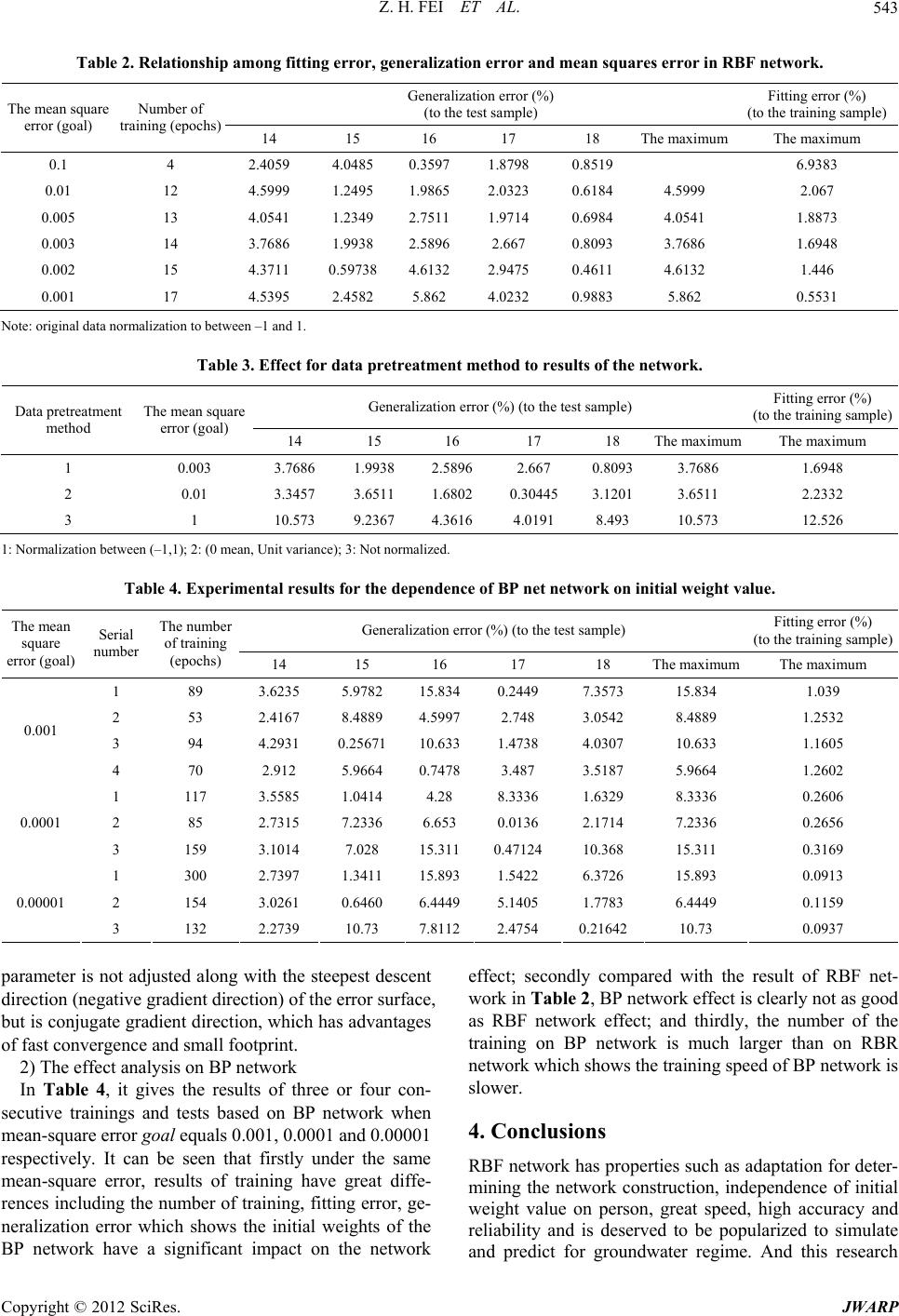

Z. H. FEI ET AL. 543
Table 2. Relationship among fitting error, generalization error and mean squares error in RBF network.
Generalization error (%)
(to the test sample) Fitting error (%) (to the training sample)
The mean square
error (goal) Number of training (epochs)14 15 16 17 18 The maximum The maximum
0.1 4 2.4059 4.0485 0.3597 1.8798 0.8519 6.9383
0.01 12 4.5999 1.2495 1.9865 2.0323 0.6184 4.5999 2.067
0.005 13 4.0541 1.2349 2.7511 1.9714 0.6984 4.0541 1.8873
0.003 14 3.7686 1.9938 2.5896 2.667 0.8093 3.7686 1.6948
0.002 15 4.3711 0.59738 4.6132 2.9475 0.4611 4.6132 1.446
0.001 17 4.5395 2.4582 5.862 4.0232 0.9883 5.862 0.5531
Note: original data normalizatio n t o between –1 and 1.
Table 3. Effect for data pretreatment method to results of the network.
Generalization error (%) (to the test sample) Fitting error (%)
(to the training sample)
Data pretreatment
method The mean square error (goal) 14 15 16 17 18 The maximum The maximum
1 0.003 3.7686 1.9938 2.5896 2.667 0.8093 3.7686 1.6948
2 0.01 3.3457 3.6511 1.6802 0.30445 3.1201 3.6511 2.2332
3 1 10.573 9.2367 4.3616 4.0191 8.493 10.573 12.526
1: Normali zation between (–1,1); 2 : (0 mean, Unit variance); 3 : Not normalized.
Table 4. Experimental results for the de pe ndence of BP net network on initial weight value.
Generalization error (%) (to the test sample) Fitting error (%)
(to the training sample)
The mean
square
error (goal)
Serial
number
The number
of training
(epochs) 14 15 16 17 18 The maximum The maximum
1 89 3.6235 5.9782 15.8340.2449 7.3573 15.834 1.039
2 53 2.4167 8.4889 4.59972.748 3.0542 8.4889 1.2532
3 94 4.2931 0.25671 10.6331.4738 4.0307 10.633 1.1605
0.001
4 70 2.912 5.9664 0.74783.487 3.5187 5.9664 1.2602
1 117 3.5585 1.0414 4.28 8.3336 1.6329 8.3336 0.2606
2 85 2.7315 7.2336 6.653 0.0136 2.1714 7.2336 0.2656 0.0001
3 159 3.1014 7.028 15.3110.47124 10.368 15.311 0.3169
1 300 2.7397 1.3411 15.8931.5422 6.3726 15.893 0.0913
2 154 3.0261 0.6460 6.44495.1405 1.7783 6.4449 0.1159 0.00001
3 132 2.2739 10.73 7.81122.4754 0.21642 10.73 0.0937
parameter is not adjusted along with the steepest descent
direction (negative gradient direction) of the error surface,
but is conjugate gradient direction, which has advantages
of fast convergence and small footprint.
2) The effect analysis on BP network
In Table 4, it gives the results of three or four con-
secutive trainings and tests based on BP network when
mean-square error goal equals 0.001, 0.0001 and 0.00001
respectively. It can be seen that firstly under the same
mean-square error, results of training have great diffe-
rences including the number of training, fitting error, ge-
neralization error which shows the initial weights of the
BP network have a significant impact on the network
effect; secondly compared with the result of RBF net-
work in Table 2, BP networ k eff ect is clearly no t as good
as RBF network effect; and thirdly, the number of the
training on BP network is much larger than on RBR
network which shows the training speed of BP network is
slower.
4. Conclusions
RBF network has prop erties such as adaptation fo r deter-
mining the network construction, independence of initial
weight value on person, great speed, high accuracy and
reliability and is deserved to be popularized to simulate
and predict for groundwater regime. And this research

Z. H. FEI ET AL. 544
shows that special attention is paid to the pretreatment of
the original data in order to have an efficient network
when we simulate and predict for groundwater dynamics
based on RBF networ k.
At the same time, drawbacks on BP network such as
artificiality for determining the construction, inferiority
to RBF net on accuracy and speed of training and ran-
dom of initial weight value to the outcome are all mani-
fested after comparing RBF net and BP net. In addition,
the BP network has many defects such as easiness to get
the local minimum when learning and volatile, and re-
dundant network connection or nodes. Many attempts
have been done to improve it, but rarely desirable result
is gotten. So we think that it should be very careful to
select the BP network to simulate and forecast ground-
water dynamics.
REFERENCES
[1] S. Cong, “The Function Analysis and Application Study
of Radial Basics Function Network,” Computer Engi-
neering and Applications, Vol. 38, No. 3, 2002, pp. 85-
87.
[2] H. Demuth and M. Beale, “Neural Network Toolbox
User’s Guide,” The MathWorks Inc., Natick, 1997, pp.
420-467.
[3] P. D. Wasserman, “Advanced Methods in Neural Com-
puting,” Van Norstrand Reinhold, New York, 1993, pp.
334-366.
[4] S.-Y. Zheng, Z.-B. Li and X.-A. Li, “Artificial Neural
Network Method for Forecast of Underground Water
Level,” Northwest Water Lou Shuntian, Shi Yang, Sys-
tems Analysis and Design Based on MATLAB-Artificial
Neural Network, XiDian University Publishing Company,
Xi’an, 1998, pp. 210-256.
[5] D. Xu and Z. Wu, “Systems Analysis and Design Based
on MATLAB6.x-Artificial Neural Network,” XiDian
University Publishing Company, Xi’an, 2002, pp. 125-
168.