 Journal of Water Resource and Protection, 2012, 4, 528-539 http://dx.doi.org/10.4236/jwarp.2012.47062 Published Online July 2012 (http://www.SciRP.org/journal/jwarp) Multistep-Ahead River Flow Prediction Using LS-SVR at Daily Scale Parag P. Bhagwat, Rajib Maity Department of Civil Engineering, Indian Institute of Technology, Kharagpur, India Email: rajib@civil.iitkgp.ernet.in Received April 5, 2012; revised May 5, 2012; accepted June 1, 2012 ABSTRACT In this study, potential of Least Square-Support Vector Regression (LS-SVR) approach is utilized to model the daily variation of river flow. Inherent complexity, unavailability of reasonably long data set and heterogeneous catchment response are the couple of issues that hinder the generalization of relationship between previous and forthcoming river flow magnitudes. The pr oblem complexity may ge t enhanced with the influence of upstream dam releases. These issues are investigated by exploiting the capability of LS-SVR—an approach that considers Structural Risk Minimization (SRM) against the Empirical Risk Minimization (ERM)—used by other learning approaches, such as, Artificial Neural Network (ANN). This study is conducted in upper Narmada river basin in India having Bargi dam in its catchment, constructed in 1989. The river gauging station—Sandia is located few hundred kilometer downstream of Bargi dam. The model development is carried out with pre-construction flow regime and its performance is checked for both pre- and post-construction of the dam for any perceivable difference. It is found that the performances are similar for both the flow regimes, which indicates that the releases from the dam at daily scale for this gauging site may be ignored. In order to investigate the temporal horizon over which the prediction performance may be relied upon, a multistep-ahead prediction is carried out and the model performance is found to be reasonably good up to 5-day-ahead predictions though the p erformance is decreasing with the increase in lead-time. Skills of both LS-SVR and ANN are reported and it is found that the former performs better than the latter for all the lead-times in general, and shor ter lead times in par- ticular. Keywords: Multistep-Ahead Prediction; Kernel-Based Learning; Least Square-Support Vector Regression (LS-SVR); Daily River Flow; Narmada River 1. Introduction River flow is an important component in hydrological cycle, which is directly available to the community. In hydrology, river flow plays an important role in estab- lishing some of the critical interactions that occur be- tween physical, ecological, social or economic processes. Accurate or at least reasonably reliable prediction of river flow is an important foundation for preventing flood, reducing natural disasters, and the optimum man- agement of water resource. Constructions of major and minor dams are essential in order to effective use of avai- lable water resources. This is more crucial for the mon- soon dominated countries, where most of the annu al rain- fall occurs during couple of months, and rest of the months are mostly no-rainfall months. Existence of dams adds to the complexity in th e river flow modelling, which is influenced by the releases from upstream reservoirs as well as the influence of the inputs from the catchment area between immediate downstream of the dam and the gauging site. Depending on the natural variability and complexity, traditional statistical methods, such as, transfer function model, Box-Jenkins approach etc. may be inadequate due to their underlying assumptions. As a consequence many new methodologies have been introduced to understand the variations of hydrologic variables and to predict for the future time steps. Development of different techniques to predict river flow is having a long history. Among the parametric linear approaches, Auto-Regressive Integrated Moving Average (ARIMA) model is one of the most popular approaches. Since last decade, machine learning techniques are being applied in this field. For instance, Artificial Neural Net- works (ANN), fuzzy logic, genetic programming, etc., have been widely used in the modelling and prediction of hydrologic variables. More recently, kernel-based learn- ing approaches have gained wide popularity. The statistical learning framework proposed by Vap- nik [1] led to the introduction of the Support Vector Ma- chine (SVM), which has been successfully applied for C opyright © 2012 SciRes. JWARP  P. P. BHAGWAT, R. MAITY 529 nonlinear classification and regression in learning prob- lems. Kernel based approaches are expected to perform better due its nonlinear, even smooth enough, feature space development based on the available historical re- cord. One such kernel based machines learning approach is the Least Squares-Support Vector Machine (LS-SVM) [2]. 1.1. Support Vector Machines (SVMs) and Kernel Based Learning SVMs are a kind of supervised machine learning system that use a linear high dimensional hypothesis space called feature space. These systems are trained using a learning algorithm, which is based on optimization theory. SVMs belong to a family of generalized linear classifier [3]. The SVMs can be applied to both classification and regression problems. Application of SVMs to regression problem was made in late nineties [1,4]. Popularity of SVM increases very rapidly since then in fields of text classification, pattern recognition, remote sensing and so on. The basic idea of working principle of SVMs is pro- vided by the use of kernel functions that implicitly map the data to a higher dimensional space. According to Cover’s theorem, linear solution in the higher dimen- sional feature space corresponds to a non-linear solution in the original lower dimensional input space. This makes SVM a powerful tool for solving a variety of hydrologic problems, which are non-linear in nature. There are me- thods available which use nonlinear kernels in their app- roach towards regression problems while applying SVMs. 1.2. Application of SVMs in Hydrologic Problems Application of SVMs in the field of hydrology is gaining wide popularity and the results are found to be encoura- ging. Such applications range from remotely sensed im- age classification [5], statistical downscaling [6], soil water forecasting [7], stream flow forecasting [8] and so on. Liong and Sivapragasam [9] compared SVM per- formance with other machine learning model, such as, ANN in forecasting flood stage and reported a superior performance of SVM. Bray and Han [10] used SVM for rainfall runoff modelling and that model was compared with a transfer function model. The study outlin ed a pro- mising area of research for further application of SVMs in unexplored areas. Samui [11] used LS-SVM to deter- mine evaporation loss of reservoir and it is established to be a powerful approach for the determination of evapo- ration loss. She and Basketfield [12] forecasted spring and fall season stream flows in Pacific Northwest region of US using SVM and reported superior results in fore- casting. Zhang et al. [13] studied two machine learning approaches—ANN and SVM and compared for appro- ximating the Soil and Water Assessment Tool (SWAT) model. The results showed that SVM in general exhibited better generalization ability than ANN. Khadam and Kaluarachchi [14] discussed the impact of accuracy and reliability of hydrolog ical data o n model calib ration. Th is, coupled with application of SVMs, was used to identify the faulty model calibration, which would have been undetected otherwise. Applicability of SVMs was also demonstrated in downscaling Global Circulation Models (GCMs), which are among the most advanced tools for estimating future climate change scenarios. The results presented SVMs as a compelli ng alternative to tradition al Artificial Neural Networks (ANN) to conduct climate impact studies [10,11] downscaled monthly precipitation to basin scale using SVMs and reported the results to be encouraging in their accuracy while showing large pro- mise for further applications. 1.3. Advancement of SVM Apart from the general benefit of SVM pointed out in the aforementioned studies, SVMs are sometimes criticized by its large number of parameters and high level of com- putational effort, particularly in case of large dataset. Chunking is one of the proposed remedies to the latter problem. However, according to Suyken et al. [15], it is worthwhile to investigate the possibility of simplifying the approach to the extent possible without losing the any of its advantages. Thus, they proposed a modification over the SVM approach, which essentially leads to Least Square-Support Vector Machines (LS-SVM). The main advantage of LS-SVM is in its higher com- putational efficiency than that of standard SVM method, since the training of LS-SVM requires only the solution of a set of linear equations instead of the long and com- putationally demanding quadratic programming problem involved in the standard SVM [2]. Qin et al. [16] in- vestigated the application of LS-SVM for the modelling of water vapor and carbon diox ide fluxes and they fou nd the excellent generalization property of LS-SVM and its potential for further applications in area of general hy- drology. Maity et al. [13] investigated the potential of support vector regression, which is also based on LS- SVM principle, for prediction of streamflow using en- dogenous property of the monthly time series. In this study, potential of LS-SVM for Regression (LS-SVR) is investigated for the obj ective outlined as follows. 1.4. Objective of This Study Potential of LS-SVM for Regression (LS-SVR) is ex- ploited for multistep-ahead river flow prediction at daily scale, to assess its performance with the increasing time Copyright © 2012 SciRes. JWARP  P. P. BHAGWAT, R. MAITY 530 horizon. Most of the major river basins are being po- pulated with major and minor dams. River flow mode- lling is supposed to be influenced by the effect of the release from these dams if the site location is on the downstream side of the dam. However, the effect of its existence will gradually reduce with increase of the dis- tance from the dam location. The study is carried out with observed daily river flow in the upper Narmada River basin with Sandia gauging station at the outlet. Bargi dam exists few hundred km upstream from the out- let of the watershed. Details of this dam are provided in th e “Study Area” section later. Investigation is carried out to assess the necessity of consideration of daily releases from upstream dam on the daily river flow variation at the outlet of the study area. Also, a multistep-ahead pre- diction is carried out to assess maximum temporal hori- zon over which the prediction results may be relied upon. The results are compared with the performance of neural networks approach that uses Empirical Risk Minimi- zation (ERM). 2. Methodology 2.1. Data Normalization The observed river flow data, as commonly used in data- driven models, is normalized to prevent the model from being dominated by the large values. The performance of LS-SVM with normalized input data has shown to out- perform the same with non-normalized input data [16]. Therefore, the data is normalized and finally the model outputs are back transformed to their original form by denormalisation. The normalization (also back transfor- mation) is carried out using 0.1 i y y 1.2max i i S S th i S 1 , (1) where i is the normalized data for day and is the observed value for day. i th i 2.2. Least Square-Support Vector Regression (LS-SVR) Let us consider a given training set ii i y x 1 , T i y y x y ()yf , where represents a 1 ,, in in yy n n-dimensional input vector and i is a scalar measured output, which represents system output. Subscript i indicates the training pattern. In the context of multistep- ahead river flow prediction, i is the vector comprising of th i i n-previous days normalized river flow values, i is the target river flow with certain lead-time in day(s) and subscript indicates the reference time from which n- previous days and the lead-time are counted. The goal is to construct a function x yx T yb , which represents the dependence of the output on the input . The form of this function is as follows: wx wb (2) where is known as weight vector and as bias. This regression model can be constructed using a non- linear mapping function . The function :nh is a mostly nonlinear function, which maps the data into a higher, possibly infinite, dimen- sional feature space. The main difference from the stan- dard SVM is that the LS-SVR involves equality con- straints instead of inequality constraints, and works with a least square cost function. The optimization problem and the equality constraints are defined by the following equations: 2 1 11 Minimize ,22 such that1,, N T i i T iii Je e be iN www wx e e (3) where i is the random error and is a regu- larization parameter in optimizing the trade-off between minimizing the training errors and minimizing the mo- del’s complexity. The objective is now to find the opti- mal parameters that minimize the prediction error of the regression model. The optimal model will be chosen by minimizing the cost function where the errors, i, are minimized. This formulation corresponds to the regre- ssion in the feature space and, since the dimension of the feature space is high, possibly infinite, this problem is difficult to solve. Therefore, to solve this optimization problem, the following Lagrange function is given, 1 ,,;, NT iiii i LwbeJ we be y wx wbi ei (4) The solution of above can be obtained by partially dif- ferentiating with respect to , , and , i.e. 1 0N ii i L w wx (5) 1 00 N i i L b (6) 0,1,, ii i Lei N e (7) 00,1,, T iii i Lbe yiN x wx w (8) From the set of Equations (5)-(8), and e can be eliminated and finally, the estimated values of b and i , i.e. and i bˆ , can be obtained by solving the linear system. Replacing in Equation (2 ) from Equatio n (5 ), w Copyright © 2012 SciRes. JWARP  P. P. BHAGWAT, R. MAITY 531 2 the kernel trick may be applied as follows: ,Kxx T ii x x ˆ , ii (9) Here, the kernel trick means a way to map the obser- vations to an inner product space, without actually com- puting the mapping and it is expected that the obser- vations will have meaningful linear structure in that inner product space. Thus, the resulting LS-SVR model can be expressed as 1 ˆ ˆN i Kbxx ,Kxx (10) where is a kernel function. i In comparison with some other feasible kernel fun- ctions, the RBF is a more compact and able to shorten the computational training process and improve the gene- ralization performance of LS-SVR (LS-SVM, in general), a feature of great importance in designing a model [13]. Aksornsingchai and Srinilta [17] studied support vector machine with polynomial kernel (SVM-POL), and su- pport vector machine with Radial Basis Function kernel (SVM-RBF) and found SVM-RBF is the accurate model for statistical downscaling methods. Also, many works have demonstrated the favorable performance of the ra- dial basis function [9,15]. Therefore, the radial basis fun- ction is adopted in this study. The nonlinear radial basis function (RBF) kernel is defined as: 2 2 1 i x x,e xp i Kxx (11) where is the kernel function parameter of the RBF kernel. The symbol is the norm of the vector and thus, 2 xx xx xˆ y yˆi y i is basically the Euclidean distance be- tween the vectors and i. In the context of river flow prediction, i is the new vector of previous river flow, based on which multi-step ahead prediction (i) is made with certain lead-time. i (observed) and are compared to assess the model performances. 2.3. Model Calibration and Parameter Estimation The regularization parameter determines the trade- off between the fitting error minimization and smooth- ness of the estimated function. It is not known before- hand which and 2 are the best for a particular problem to achieve maximum performance with LS-SVR models. Thus, the regularization parameter and the RBF kernel parameter 2 have to be calibrated during model development period. These parameters are inter- dependent, and their (near) optimal values are often ob- tained by a trial-and-error method. Interrelationship is also coupled with the number of previous river flow values to be considered, which is denoted as . In order to find all these parameters ( n , and ) grid search method is employed in parameter space. Once the para- meters are estimated from the training dataset, the ob- tained LS-SVR model is complete and ready to use for modelling new river flow data period. Performance of the developed model is then assessed with the data set during testing period. Different models (parameter sets) are developed for different prediction lead-times in case of multi-step ahead prediction. n 2.4. Comparison with Artificial Neural Networks (ANN) The flexible computing based ANN models have been extensively studied and used for time series forecasting in many hydrologic applications since late 1990s. This model has the capability to execute complex mapping between input and output and to form a network that approximates non-linear functions. A single hidden layer feed forward network is the most widely used model form for time series modeling and forecasting [18]. This model usually consists of three layers: the first layer is the input layer where the data are introduced to the net- work followed by the hidden layer where data are pro cessed and the final or output layer is where the results of the given input are produced. The number of input nodes and output nodes in an ANN are dependent on the problem to which the network is being applied. However, there is no fixed method to find out the number of hidden layer nodes. If there are too few nodes in the hidden layer, the network may have difficulty in generalizing the problems. On the other hand, if there are too many nodes in the hidden layer, the net- work may take an unacceptably long time to learn any thing from the training set [19]. Increase in the number of parameters may slow the calibration process [20]. In a study by Zealand et al. [21], networks were initially con figured with both one and two hidden layers. However, the improvement in forecasting results was only marginal for the two hidden layer cases. Therefore, it is decided to use a single hidden layer in this study. In most of the cases, suitable number of neurons in the hidden layer is obtained based on the trial-and-error method [22]. Maity and Nagesh Kumar, [23] proposed a GA based evolution- ary approach to decide the complete network structure. The output t of an ANN, assuming a linear output neuron having a single hidden layer with h sigmoid hidden nodes, is given by: 1 h tjjk j gwfsb (12) where and k are the linear transfer function and bias respectively of the output neuron k, b w th j is the connection weights between neuron of hidden la- Copyright © 2012 SciRes. JWARP 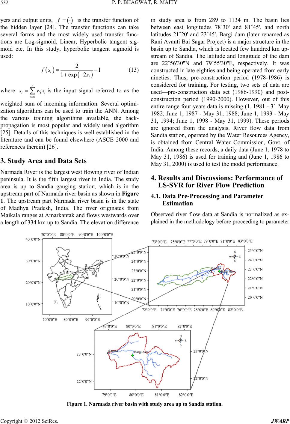 P. P. BHAGWAT, R. MAITY CopyrigSciRes. JWARP 532 f ht © 2012 yers and output units, is the transfer function of the hidden layer [24]. The transfer functions can take several forms and the most widely used transfer func- tions are Log-sigmoid, Linear, Hyperbolic tangent sig- moid etc. In this study, hyperbolic tangent sigmoid is used: in study area is from 289 to 1134 m. The basin lies between east longitudes 78˚30' and 81˚45', and north latitudes 21˚20' and 23˚45'. Bargi dam (later renamed as Rani Avanti Bai Sagar Project) is a major structure in the basin up to Sandia, which is located few hundred km up- stream of Sandia. The latitude and longitude of the dam are 22˚56'30''N and 79˚55'30''E, respectively. It was constructed in late eighties and being operated from early nineties. Thus, pre-construction period (1978-1986) is considered for training. For testing, two sets of data are used—pre-construction data set (1986-1990) and post- construction period (1990-2000). However, out of this entire range four year s data is missing (1, 1981 - 31 May 1982; June 1, 1987 - May 31, 1988; June 1, 1993 - May 31, 1994; June 1, 1998 - May 31, 1999). These periods are ignored from the analysis. River flow data from Sandia station, operated by the Water Resources Agency, is obtained from Central Water Commission, Govt. of India. Among these records, a daily data (June 1, 1978 to May 31, 1986) is used for training and (June 1, 1986 to May 31, 2000) is used to test the model performance. 21 xp2 i s i i 1e i fs (13) 0 n i i wx where is the input signal referred to as the weighted sum of incoming information. Several optimi- zation algorithms can be used to train the ANN. Among the various training algorithms available, the back- propagation is most popular and widely used algorithm [25]. Details of this techniques is well established in the literature and can be found elsewhere (ASCE 2000 and references therein) [26]. 3. Study Area and Data Sets Narmada River is the largest west flowing river of Indian peninsula. It is the fifth largest river in India. The study area is up to Sandia gauging station, which is in the upstream part of Narmada river basin as shown in Figure 1. The upstream part Narmada river basin is in the state of Madhya Pradesh, India. The river originates from Maikala ranges at Amarkantak and flows westwards over a length of 334 km up to Sandia. The elevation difference 4. Results and Discussions: Performance of LS-SVR for River Flow Prediction 4.1. Data Pre-Processing and Parameter Estimation Observed river flow data at Sandia is normalized as ex- plained in the methodology before proceeding to parameter Figure 1. Narmada river basin with study area up to Sandia station. 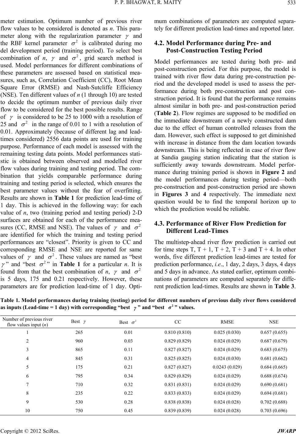 P. P. BHAGWAT, R. MAITY 533 meter estimation. Optimum number of previous river flow values to be considered is denoted as n. This para- meter along with the regularization parameter and the RBF kernel parameter 2 is calibrated during mo del development period (training period). To select best combination of n, and 2 , grid search method is used. Model performances for different combinations of these parameters are assessed based on statistical mea- sures, such as, Correlation Coefficient (CC), Root Mean Square Error (RMSE) and Nash-Sutcliffe Efficiency (NSE). Ten different values of n (1 through 10) are tested to decide the optimum number of previous daily river flow to be considered for the best possible results. Range of is considered to be 25 to 1000 with a resolution of 25 and 2 in the range of 0.01 to 1 with a resolution of 0.01. Approximately (because of different lag and lead- times considered) 2556 data points are used for training purpose. Performance of each model is assessed with the remaining testing data points. Model performances stati- stic is obtained between observed and modelled river flow values during training and testing period. The com- bination that yields comparable performance during training and testing period is selected, which ensures the best parameter values without the fear of overfitting. Results are shown in Table 1 for prediction lead-time of 1 day. This is achieved in the following way: for each value of n, two (training period and testing period) 2-D surfaces are obtained for each of the performance mea- sures (CC, RMSE and NSE). The values of and 2 are identified for which the training and testing period performances are “closest”. Priority is given to CC and corresponding RMSE and NSE are reported for same values of and 2 . These values are named as “best ” and “best 2 ” in Table 1 for a particular n. It is found from that the best combination of n, and 2 is 5 days, 175 and 0.21 respectively. However, these parameters are for prediction lead-time of 1 day. Opti- mum combinations of parameters are computed separa- tely for different prediction lead-times and reported later. 4.2. Model Performance during Pre- and Post-Construction Testing Period Model performances are tested during both pre- and post-construction period. For this purpose, the model is trained with river flow data during pre-construction pe- riod and the developed model is used to assess the per- formance during both pre-construction and post con- struction period. It is found that the performance remains almost similar in both pre- and post-construction period (Table 2). Flow regimes are supposed to be modified on the immediate downstream of a newly constructed dam due to the effect of human controlled releases from the dam. However, such effect is supposed to get diminished with increase in distance from the dam location towards downstream. This is being reflected in case of river flow at Sandia gauging station indicating that the station is sufficiently away towards downstream. Model perfor- mance during training period is shown in Figure 2 and the model performances during testing period—both pre-construction and post-construction period are shown in Figures 3 and 4 respectively. The immediate next question would be to find the temporal horizon up to which the prediction would be reliable. 4.3. Performance of River Flow Prediction for Different Lead-Times The multistep-ahead river flow prediction is carried out for time steps T, T + 1, T + 2, T + 3 and T + 4. In other words, five different prediction lead-times are tested for prediction performance, i.e., 1 day, 2 days, 3 days, 4 days and 5 days in advance. As stated earlier, optimum combi- nations of parameters are computed separately for diffe- rent prediction lead-times. Results are shown in Table 3 . Table 1. Model performances during training (testing) period for different numbers of previous daily river flows considered as inputs (Lead-time = 1 day) wi th corre sponding “be st ” and “best ” values. 2 σ Number of previous river flow values input (n) Best Best 2 CC RMSE NSE 1 265 0.01 0.810 (0.810) 0.025 (0.030) 0.657 (0.655) 2 960 0.03 0.829 (0.829) 0.024 (0.029) 0.687 (0.679) 3 865 0.11 0.827 (0.827) 0.024 (0.029) 0.683 (0.675) 4 845 0.31 0.825 (0.825) 0.024 (0.030) 0.681 (0.662) 5 175 0.21 0.827 (0.827) 0.0243 (0.029) 0.684 (0.665) 6 795 0.34 0.829 (0.829) 0.024 (0.029) 0.688 (0.674) 7 710 0.32 0.831 (0.831) 0.024 (0.029) 0.690 (0.681) 8 235 0.22 0.833 (0.833) 0.024 (0.029) 0.694 (0.681) 9 530 0.28 0.838 (0.838) 0.024 (0.028) 0.702 (0.688) 10 750 0.45 0.839 (0.839) 0.024 (0.028) 0.703 (0.696) Copyright © 2012 SciRes. JWARP 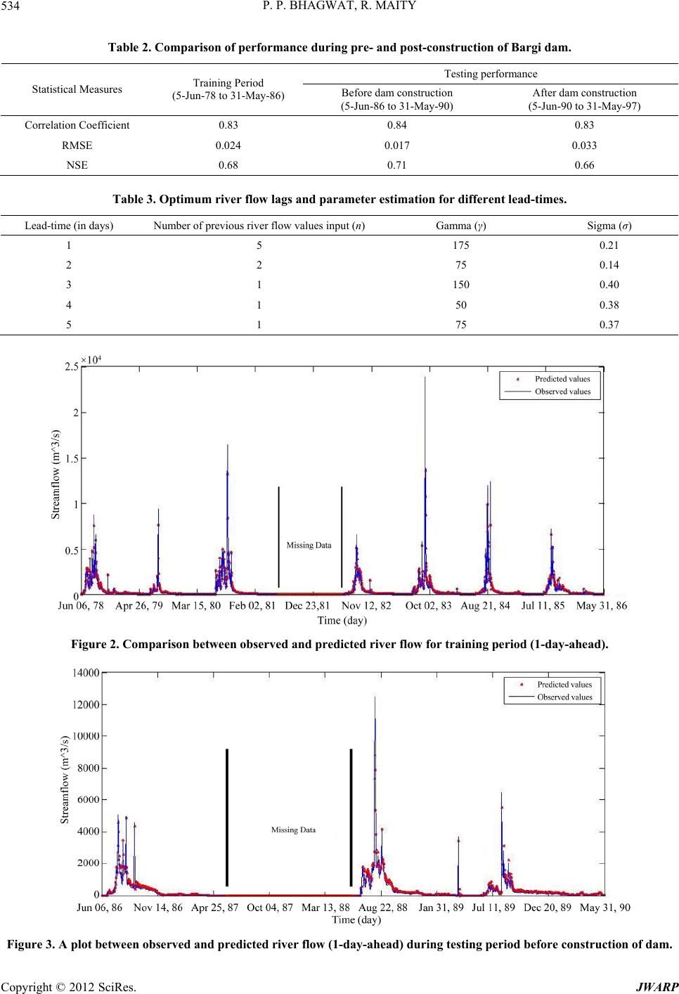 P. P. BHAGWAT, R. MAITY 534 Table 2. Comparison of performance during pre- and post-c onstr uc tion of Bar g i dam. Testing performance Statistical Measures Training Period (5-Jun-78 to 31-May-86) Before dam const ruc ti on (5-Jun-86 to 31-May-90) After dam construction (5-Jun-90 to 31-May-97) Correlation Coefficient 0.83 0.84 0.83 RMSE 0.024 0.017 0.033 NSE 0.68 0.71 0.66 Table 3. Optimum river flow lags and parameter estimation for different lead-times. Lead-time (in days) Number of previous river flow value s input (n) Gamma (γ) Sigma (σ) 1 5 175 0.21 2 2 75 0.14 3 1 150 0.40 4 1 50 0.38 5 1 75 0.37 Figure 2. Comparison between observed and predicted river flow for training period (1-day-ahead). Figure 3. A plot between observed and predicted river flow (1-day-ahead) during testing period before construction of dam. Copyright © 2012 SciRes. JWARP 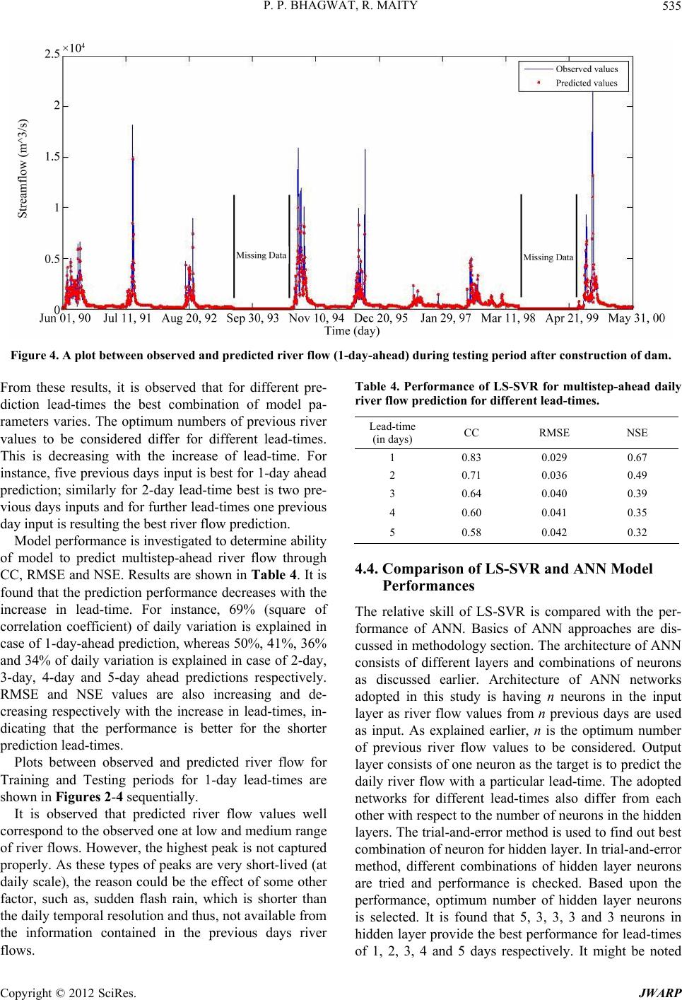 P. P. BHAGWAT, R. MAITY Copyright © 2012 SciRes. JWARP 535 Figure 4. A plot between observed and predicted river flow (1-day-ahead) during testing period after construction of dam. Table 4. Performance of LS-SVR for multistep-ahead daily river flow prediction for different lead-times. From these results, it is observed that for different pre- diction lead-times the best combination of model pa- rameters varies. The optimum numbers of previous river values to be considered differ for different lead-times. This is decreasing with the increase of lead-time. For instance, five previous days input is best for 1-day ahead prediction; similarly for 2-day lead-time best is two pre- vious days inputs and for further lead-times one previous day input is resulting the best river flow prediction. Lead-time (in days) CC RMSE NSE 1 0.83 0.029 0.67 2 0.71 0.036 0.49 3 0.64 0.040 0.39 4 0.60 0.041 0.35 5 0.58 0.042 0.32 Model performance is investigated to determine ability of model to predict multistep-ahead river flow through CC, RMSE and NSE. Results are shown in Table 4. It is found that the prediction performance decreases with the increase in lead-time. For instance, 69% (square of correlation coefficient) of daily variation is explained in case of 1-day-ahead prediction, whereas 50%, 41%, 36% and 34% of daily variation is explained in case of 2-day, 3-day, 4-day and 5-day ahead predictions respectively. RMSE and NSE values are also increasing and de- creasing respectively with the increase in lead-times, in- dicating that the performance is better for the shorter prediction lead-times. 4.4. Comparison of LS-SVR and ANN Model Performances The relative skill of LS-SVR is compared with the per- formance of ANN. Basics of ANN approaches are dis- cussed in methodology section. The architecture of ANN consists of different layers and combinations of neurons as discussed earlier. Architecture of ANN networks adopted in this study is having n neurons in the input layer as river flow values from n previous days are used as input. As explained earlier, n is the optimum number of previous river flow values to be considered. Output layer consists of one neuron as the target is to predict the daily river flow with a particular lead-time. The adopted networks for different lead-times also differ from each other with respect to the number of neuron s in the hi dden layers. The trial-and-error method is used to find out best combination of neur on for h idden layer. In trial-and-error method, different combinations of hidden layer neurons are tried and performance is checked. Based upon the performance, optimum number of hidden layer neurons is selected. It is found that 5, 3, 3, 3 and 3 neurons in hidden layer provid e the best performance for lead-times of 1, 2, 3, 4 and 5 days respectively. It might be noted Plots between observed and predicted river flow for Training and Testing periods for 1-day lead-times are shown in Figures 2-4 sequentially. It is observed that predicted river flow values well correspond to the observed one at low and medium range of river flows. However, the highest peak is not captured properly. As these types of peaks are very short-lived (at daily scale), the reason could be the effect of some other factor, such as, sudden flash rain, which is shorter than the daily temporal resolution and thus, not available from the information contained in the previous days river flows.  P. P. BHAGWAT, R. MAITY 536 here that back propagation algorithm (as explained ear- lier) is used to train these networks using 2556 to 2552 (from lead-time 1-day through 5-day) training data set. The largest network (5-5-1) is having 25 + 5 + 5 + 1 = 31 parameters, which is much less than number of training patterns. Different networks for different lead-times are trained separately. Statistical measures showing the prediction performances are obtained during training and testing period for different lead-time cases and the results are shown in Table 5. After comparison between LS-SVR and ANN, it is found that, in general, LS-SVR performs better than ANN for all the lead-times. For instance, at 1-day lead-time, 69% (CC = 0.83) and 53.2% (CC = 0.73) of daily river flow variation are captured by LS-SVR and ANN respectively dur ing the entire testing period (Table 5). Also, for this case, the NSE values are found to be 0.67 and 0.52 in case of LS-SVR and ANN respectively. The performance of ANN also decreases with the in- crease in lead-time. It is also found that the difference in prediction performance obtained from LS-SVR and ANN is more prominent for shorter lead times. As the lead time increases, the performance of LS-SVR and ANN becomes comparable. Different error measures, i.e., Mean Absolute Error (MAE), Mean Absolute Relative Error (MARE) and Root Mean Square Error (RMSE) are also determined for LS-SVR and ANN based predictions. Results are shown in Table 6. Based on these measures also, it is found that error measures for LS-SVR are bet- ter compared to that of ANN. These observations indi- cate the higher capability of LS-SVR approach to capture the river flow variation using the previous inf ormation. For a visual comparison of prediction performances by LS-SVR and ANN simultaneously, both LS-SVR and ANN model predicted river flow values are plotted with the observed river flow during the model testing period (Figure 5). This is shown in case of 1-day-ahead prediction—best for both LS-SVR and ANN. It is ob- served that predicted river flow values are very well corresponds to the low and medium range of river flow in case of LS-SVR and ANN. Relatively better perfor- mance of LS-SVR is discussed with respect to the sta- tistical measures as shown in Table 5. However, as discussed in case of LS-SVR earlier, the peak river flow values are not captured with reasonable accuracy in case of ANN as well. Apart from the fact that these peaks are very short-lived (at daily scale), this is a shortcoming for both LS-SVR and ANN based approaches. The reason could be the same as discussed before, i.e., these peaks might be the effect of some factor, such as, sudden flash rain, which is shorter than the daily temporal resolution and thus, not available from the information contained in the previous days river flows alone. Consideration and incorporation of such additional inputs could be future scope of study. However, the better performance of LS- SVR, particularly for shorter prediction lead-times, as compared to that of ANN, is noticed in this study. The better performance of LS-SVR over ANN may be Table 5. Performance measures for LS-SVR and ANN models for training and testing period (1978-2000). Testing period values are shown within parentheses. LS-SVR ANN Lead-time (in days) Optimum number of previous daily flow(s) to be considered CC NSE CC NSE 1 5 0.83 (0.83) 0.68 (0.67) 0.76 (0.73) 0.58 (0.52) 2 2 0.71 (0.71) 0.51 (0.49) 0.71 (0.71) 0.50 (0.49) 3 1 0.64 (0.64) 0.40 (0.39) 0.63 (0.59) 0.39 (0.33) 4 1 0.61 (0.60) 0.36 (0.35) 0.66 (0.55) 0.43 (0.30) 5 1 0.58 (0.58) 0.33 (0.32) 0.62 (0.56) 0.39 (0.30) CC: Correlation Coefficient; NSE: Nash-Sutcliffe Efficiency (NSE). Table 6. Error measures for LS-SVR and ANN models for training and testing period. Testing period values are shown within parentheses. LS-SVR ANN Lead-time (in days) MAE MARE RMSE MAE MARE RMSE 1 0.006 (0.008) 0.031 (0.041) 0.024 (0.029) 0.008 (0.009) 0.055 (0.049) 0.028 (0.035) 2 0.008 (0.010) 0.044 (0.059) 0.030 (0.036) 0.008 (0.010) 0.047 (0.056) 0.031 (0.036) 3 0.009 (0.012) 0.056 (0.065) 0.033 (0.040) 0.009 (0.011) 0.053 (0.058) 0.034 (0.042) 4 0.011 (0.012) 0.066 (0.070) 0.034 (0.041) 0.010 (0.012) 0.061 (0.061) 0.033 (0.043) 5 0.011 (0.013) 0.069 (0.073) 0.035 (0.042) 0.010 (0.012) 0.060 (0.067) 0.034 (0.042) MAE: Mean Absolute Error; MARE: Mean Absolute Relative Error; RMSE : Root Mean Square Error. Copyright © 2012 SciRes. JWARP  P. P. BHAGWAT, R. MAITY 537 Figure 5. Comparison between observed and predicted river flow from LS-SVR and ANN (1-day-ahead). attributed to its fundamental approach towards error mi- nimization. Fundamental difference in the working prin- ciples of ANN and LS-SVR (SVM, in general) lies in their approaches of risk minimization. ANN follows an Empirical Risk Minimization (ERM) approach, whereas Structural Risk Minimization (SRM) principle is fol- lowed in LS-SVR. The SRM minimizes an upper bound on the generalization error, as opposed to ERM which minimizes the error on the training data. Thus, the solu- tions may fall in to local optima in case of ANN [27]. It is this difference which equips LS-SVR with a greater potential to generalize the regression surface without the danger of overfitting the training data set and global opti- mum solution is guaranteed in LS-SVR [28]. With respect to the number of parameters, LS-SVR is less complex than ANN. As discussed earlier, there are only three parameters in LS-SVR based approach, namely—regularization parameter ( ) RBF kernel pa- rameter ( ) and number of previous daily river flow values to be considered (n). However, in ANN, the num- ber of hidden layers, number of hidden nodes, transfer functions and so on must be determined, which are com- paratively more complex. On the other hand, LS-SVR is able to provide better prediction with small sample size. This is because the decision function of LS-SVR is only determined by supporting vectors. In general, the su- pporting vectors are only a part of training pattern (from available river flow data) and the remaining pattern are not used in constructing the LS-SVR model. Therefore the performance of LS-SVR may still be acceptable, even if the sample size is small. In contrast, the decision fun- ction in ANN is determined by all training data sets [29]. Thus, generalization of relationship between past and future river flow values is more likely in case of LS-SVR as found in this study and thus, more suitable for mul- tistep-ahead prediction. 5. Conclusions In this study, daily variation of river flow is modelled and potential Least Square-Support Vector Regression (LS-SVR) is used for multistep-ahead river flow predic- tion. Daily river flow values from Sandia station at upper Narmada river basin in India are used for illustration. Bargi dam is located few hundred km upstream of Sandia. It is investigated whether it is required to consider the releases from the upstream dam to model the daily varia- tion at Sandia. Parameters of LS-SVR – (regulariza- tion parameter) and (RBF kernel parameter) and optimum numbers of previous river flow values to be considered (n) are estimated based on the model per- formance during model development period (June 1, 1978 to May 31, 1986 excluding the missing data). The model is tested for the period June 1, 1986 to May 31, 2000 and different statistical performance measures (CC, NSE, RMSE, MAE and MARE) are obtained. These sta- tistical measures confirm the well correspondence be- tween observed and predicted river flow values. This correspondence is found to be better for low and medium range of flow values. However, the peak river flow va- lues are not captured with reasonable accuracy in case of both LS-SVR and ANN. While comparing the performance during pre- and post-construction of dam, it is found that the prediction performances are similar for both the flow regimes, which indicates that we may ignore the releases from the dam at daily scale for this gauging site. In order to inves- tigate the temporal horizon over which this may be relied upon, a multistep-ahead prediction is carried out and the model performance is investigated up to 5-day-ahead Copyright © 2012 SciRes. JWARP  P. P. BHAGWAT, R. MAITY 538 predictions. The performance is found to be decrease with the increase in lead-time. In other words, the per- formance is better for shorter lead-times. General comparison between LS-SVR and ANN mo- del reveals that the performance of LS-SVR is better that that of ANN for all the lead-times—1-d ay-ahead through 5-day-ahead prediction. Better performance of LS-SVR, in comparison with that of ANN, becomes more pro- minent for shorter prediction lead-times. Thus, the better performance of LS-SVR, as compared to that of ANN, is noticed for multistep-ahead prediction. The superior per- formance of LS-SVR over ANN may be attributed to its fundamental approach towards error minimization, en- sured global optimum solution and capability to gene- ralize the relationship between past and future river flow values, even with short length of available data. Thus, it may be inferred that Structural Risk Minimization (SRM) is better approach as compared to Empirical Risk Mini- mization (ERM) and LS-SVR, being a SRM based app- roach, may be used for multistep-ahead prediction to obtain better performance. Use of exogenous inputs may be of further research interests. REFERENCES [1] V. N. Vapnik, “Statistical Learning Theory,” John Wiley and Sons, New York, 1998. [2] J. A. K. Suykens and J. Vandewalle, “Least Squares Support Vector Machine Classifiers,” Neural Processing Letters, Vol. 9, No. 3, 1999, pp. 293-300. doi:10.1023/A:1018628609742 [3] B. E. Boser, I. Guyon and V. Vapnik, “A Training Algo- rithm for Optimal Margin Classifiers,” Proceedings Fifth Annual Workshop on Computational Learning Theory, Pittsburgh, 1992, pp. 144-152. [4] H. D. Drucker, C. J. C. Burges, L. Kaufman, A. Smola and V. Vapnik, “Support Vector Regression Machines,” In: M. C. Mozer, M. I. Jordan and T. Petsche, Eds., Ad- vances in Neural Information Processing Systems, Vol. 9, Morgan Kaufmann, San Mateo, 1997, pp. 155-161. [5] Y. B. Dibike, S. Velickov, D. Slomatine and M. B. Ab- bott, “Model Induction with Support Vector Machines: Introduction and Applications,” Journal of Computing in Civil Engineering, Vol. 15, No. 3, 2001, pp. 208-216. doi: 10.1061/(ASCE)0887-3801(2001)15:3(208) [6] S. Tripathi, V. V. Srinivas and R. S. Nanjundian, “Down- scaling of Precipitation for Climate Change Scenarios: A Support Vector Machine Approach,” Journal of Hydrol- ogy, Vol. 330 No. 3-4, 2006, pp. 621-640. doi: 10.1016/j.jhydrol.2006.04.030 [7] W. Wu, X. Wang, D. Xie and H. Liu, “Soil Water Con- tent Forecasting by Support Vector Machine in Purple Hilly Region,” International Federation for Information Processing, Vol. 258, 2008, pp. 223-230. doi:10.1007/978-0-387-77251-6_25 [8] R. Maity, P. P. Bhagwat and A. Bhatnagar, “Potential of Support Vector Regression for Prediction of Monthly Streamflow Using Endogenous Property,” Hydrological Processes, Vol. 24, No. 7, 2010, pp. 917-923. doi: 10.1002/hyp.7535 [9] S.-Y. Liong and C. Sivapragasam, “Flood Stage Forecas- ting with Support Vector Machines,” Journal of the Ame- rican Water Resources Association, Vol. 38, No. 1, 2002, pp. 173-196. doi:10.1111/j.1752-1688.2002.tb01544.x [10] M. Bray and D. Han, “Identification of Support Vector Machines for Runoff Modelling,” Journal of Hydroin- formatics, Vol. 6, No. 4, 2004, pp. 265-280. [11] P. Samui, “Application of Least Square Support Vector Machine (LSSVM) for Determination of Evaporation Losses in Reservoirs,” Engineering, Vol. 3, No. 4, 2011, pp. 431-434. doi:10.4236/eng.2011.34049 [12] N. She and D. Basketfield, “Long Range Forecast of Stream Flow Using Support Vector Machine,” Proceed- ings of the World Water and Environment Resources Congress, ASCE, Anchorage, 2005. doi:10.1061/40792(173)481 [13] X. Zhang, R. Srinivasan and M. V. Liew, “Approxi- mat- ing SWAT Model Using Artificial Neural Network and Support Vector Machine,” Journal of the American Water Resources Association, Vol. 45, No. 2, 2009, pp. 460-474. doi:10.1111/j.1752-1688.2009.00302.x [14] I. M. Khadam and J. J. Kaluarachchi, “Use of Soft Infor- mation to Describe the Relative Uncertainty of Calibra- tion Data in Hydrologic Models,” Water Resources Re- search, Vol. 40, No. W11505, 2004, p. 15. doi: 10.1029/2003WR002939 [15] J. A. K. Suykens, J. De Brabanter, L. Lukas and J. Vandewalle, “Weighted Least Squares Support Vector Machines: Robustness and Sparse Approximation,” Neu- rocomputing, Vol. 48, No. 1-4, 2002, pp. 85-105. doi:10.1016/S0925-2312(01)00644-0 [16] Z. Qin, Q. Yu, J. Li, Z. Wu and B. Hu, “Application of Least Squares Vector Machines in Modelling Water Va- por and Carbon Dioxide Fluxes over a Cropland,” Jour- nal of Zhejiang University Science, Vol. B6, No. 6, 2005, pp. 491-495, doi: 10.1631/jzus.2005.B0491 [17] P. Aksornsingchai and C. Srinilta, “Statistical Down- scaling for Rainfall and Temperature Prediction in Thai- land,” Proceeding of the International MultiConference of Engineers and Computer Scientists, Hong Kong, Vol. 1, 16-18 March 2011. [18] G. Zhang, B. E. Patuwo and M. Y. Hu, “Forecasting with Artificial Neural Networks: The State of the Art,” Inter- national Journal of Forecasting, Vol. 14, No. 1, 1998, pp. 35-62. doi:10.1016/S0169-2070(97)00044-7 [19] T. Naes, K. Kvaal, T. Isaksson and C. Miller, “Artificial Neural Networks in Multivariate Calibration,” Journal of Near-Infrared Spectroscopy, Vol. 1, 1993, pp. 1-11. doi:10.1255/jnirs.1 [20] A. Y. Shamseldin, “Application of a Neural Network Technique to Rainfall-Runoff Modeling,” Journal of Hy- drology, Vol. 199, No. 3, 1997, pp. 272-294. [21] C. M. Zealand, D. H. Burn and S. P. Simonovic, “Short Term Stream Flow Forecasting Using Artificial Neural Copyright © 2012 SciRes. JWARP  P. P. BHAGWAT, R. MAITY Copyright © 2012 SciRes. JWARP 539 Networks,” Journal of Hydrology, Vol. 214, No. 1-4, 1999, pp. 32-48. doi:10.1016/S0022-1694(98)00242-X [22] A. S. Weigend, D. E. Rumelhart and B. A. Huberman, “Predicting the Future: A Connectionist Approach,” In- ternational Journal of Neural Systems, Vol. 1, No. 3, 1992, pp. 193-209. [23] R. Maity and D. Nagesh Kumar, “Basin-Scale Stream Flow Forecasting Using the Information of Large-Scale Atmospheric Circulation Phenomena,” Hydrological Pro- cesses, Vol. 22, No. 5, 2008, pp. 643-650. doi:10.1002/hyp.6630 [24] P. Coulibaly and N. D. Evora, “Comparison of Neural Network Methods for Infilling Missing Daily Weather Records,” Journal of Hydroogy, Vol. 341, No. 1-2, 2007, pp. 27-41. doi:10.1016/j.jhydrol.2007.04.020 [25] H. F. Zou, G. P. Xia, F. T. Yang and H. Y. Wang, “An Investigation and Comparison of Artificial Neural Net- work and Time Series Models for Chinese Food Grain Price Forecasting,” Neurocomputing, Vol. 70, No. 16-18, 2007, pp. 2913-2923. doi:10.1016/j.neucom.2007.01.009 [26] ASCE, “Artificial Neural Networks in Hydrology. II: Hydrologic Applications,” ASCE Task Committee on Application of Artificial Neural Networks in Hydrology, Journal of Hydrologic Engineering, Vol. 5, No. 2, 2000, pp. 124-137. doi:10.1061/(ASCE)1084-0699(2000)5:2(124) [27] T. Van Gestel, J. A. K. Suykens, B. Baesens, S. Viaene, J. Vanthienen, G. Dedene, B. De Moor and J. Vandewalle, “Benchmarking Least Squares Support Vector Machine Classifiers,” Machine Learning, Vol. 54, No. 1, 2004, pp. 5-32. doi:10.1023/B:MACH.0000008082.80494.e0 [28] W. H. Chen, J. Y. Shih and S. Wu, “Comparison of Sup- port-Vector Machines and Back Propagation Neural Networks in Forecasting the Six Major Asian Stock Mar- kets,” International Journal of Electronic Finance, Vol. 1, No. 1, 2006 , pp. 49-67. [29] R. M. Balabin and E. I. Lomakina, “Support Vector Ma- chine Regression (LS-SVM)—An Alternative to Artifi- cial Neural Networks (ANNs) for the Analysis of Quan- tum Chemistry Data?” Physical Chemistry Chemical Phy- sics, Vol. 13, No. 24, 2011, pp. 11710-11718. doi:10.1039/c1cp00051a
|