 Journal of Water Resource and Protection, 2012, 4, 439-450 http://dx.doi.org/10.4236/jwarp.2012.47051 Published Online July 2012 (http://www.SciRP.org/journal/jwarp) Calibration of SWAT2009 Using Crop Biomass, Evapotranspiration, and Deep Recharge: Calera Watershed in Zacatecas, Mexico Case Study Jose R. Ávila-Carrasco1, Francisco Mojarro Dávila1*, Daniel N. Moriasi2, Prasanna H. Gowda3, Carlos Bautista-Capetillo1, Francisco G. Echavarria-Cháirez4, Jurgen D. Garbrecht2, Jean L. Steiner2, Terry A. Howell3, Edward T. Kanemasu5, Alan J. Verser2, Kev in Wagner6, Jairo Hernandez7 1Universidad Autónoma de Zacatecas, Zacatecas, México 2USDA-ARS-Grazinglands Research Laboratory, El Reno, USA 3USDA-ARS-Conservation and Production Research Laboratory, Bushland, USA 4Instituto Nacional de Investigaciones Forestales Agricolas y Pecuarias (INIFAP), Zacatecas Calera de V.R., Mexico 5Office of Global Programs, University of Georgia, Georgia, USA 6Texas Water Resources Institute, Texas A&M Institute of Renewable Natural Resources, College Station, USA 7Department of Civil Engineering, Boise State University, Boise, USA Email: *mojarro_fr@yahoo.com.mx Received April 6, 2012; revised May 3, 2012; accepted June 1, 2012 ABSTRACT Groundwater is the main source of water in the semi-arid Calera watershed, located in the State of Zacatecas, Mexico. Due to increasing population, rapid industrial growth, and increased irrigation to meet growing food demand, ground- water extraction in the Calera watershed are exceeding recharge rates. Therefore, development and evaluation of alter- native water management strategies are needed for sustainable development of the region. The Soil and Water Assess- ment Tool (SWAT) model was selected for this purpose as it has been used to simulate a wide range of agricultural production, the extensive testing and application in diverse watersheds worldwide, and the potential for future linkage of this model to groundwater models. However, crucial flow data which are commonly used for calibrating hydrologic models are not available in this watershed. This paper describes a novel calibration methodology that uses biomass and water balance approach which has potential for calibration of hydrologic models in ungauged or data-scarce watersheds, which are prevalent in many parts of the world. Estimated long-term annual average actual evapotranspiration (AET), and deep aquifer recharge rates and plant biomass values based on the expert knowledge of researchers and managers in the watershed were used as targets for calibration. The model performance was assessed using the Nash-Sutcliffe effi- ciency coefficient (NSE), coefficient of determination (R2), and percent bias (PBIAS, %) statistics. On average, the ca- librated SWAT model yielded annual Nash-Sutcliffe efficiency coefficient values of 0.95, 0.99, and 0.85 for AET, re- charge, and biomass, respectively. The coefficient of determination, values for AET, recharge, and biomass were 0.95, 0.94, and 0.99 respectively. The percent bias values of ±2.21%, ±0.18%, and ±0.96% for AET, recharge, and biomass, respectively, indicated that the model reproduced the calibration target values of the three water budget variables within an acceptable value of ±10.0%. Therefore, it is concluded that the calibrated SWAT model can be used in evaluating alternative water management scenarios for the Calera watershed without further validation. Considering the relative ease in developing calibration data and excellent performance statistics, the calibration methodology proposed in this study may have the potential to be used for ungauged or data-scare agricultural watersheds that are prevalent in many parts of the world. Keywords: SWAT; Calera Watershed; Scenarios; Recharge; Evapotranspiration; Runoff; Erosion 1. Introduction Underlying unconfined Calera aquifer is the primary source of water in the semi-arid Calera watershed, lo- cated in the most populated, economical and industria- lized part of the state of Zacatecas, Mexico. Municipali- ties within the Calera Watershed account for about 60% of the state population and about 80% of the Calera re- gion population live in urban areas. Calera watershed provides 74% of the state’s (GDP) (gross domestic pro- duct), and generate 17% of employment [1] with irri- gated agriculture being the largest employer followed by commerce, mining, livestock, and industry [2]. The ma- *Corresponding author. C opyright © 2012 SciRes. JWARP 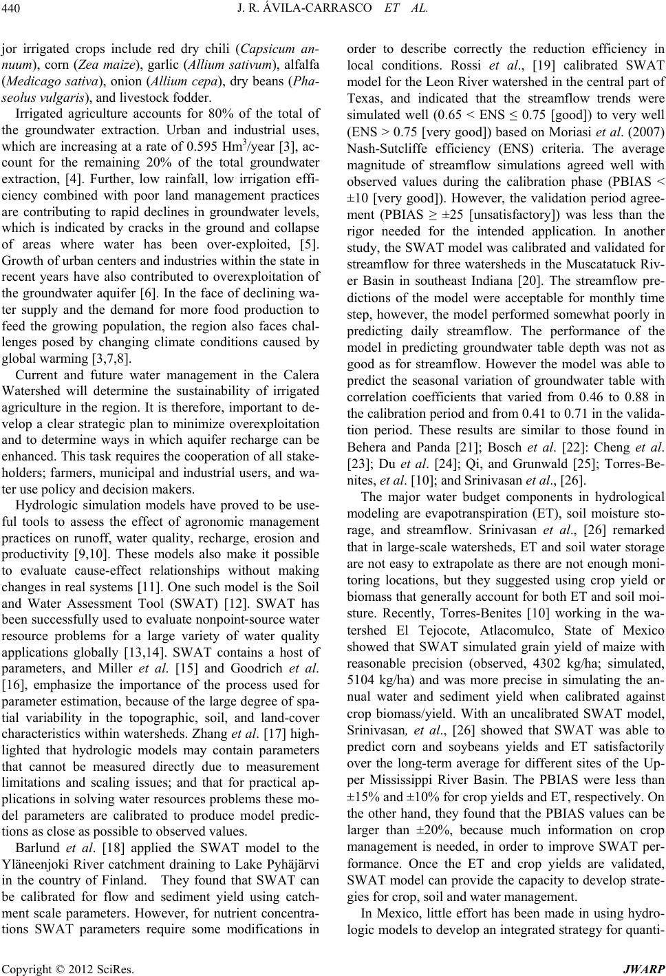 J. R. ÁVILA-CARRASCO ET AL. 440 jor irrigated crops include red dry chili (Capsicum an- nuum), corn (Zea maize), garlic (Allium sativum), alfalfa (Medicago sativa), onion (Allium cepa), dry beans (Pha- seolus vulgaris), and livestock fodder. Irrigated agriculture accounts for 80% of the total of the groundwater extraction. Urban and industrial uses, which are increasing at a rate of 0.595 Hm3/year [3], ac- count for the remaining 20% of the total groundwater extraction, [4]. Further, low rainfall, low irrigation effi- ciency combined with poor land management practices are contributing to rapid declines in groundwater levels, which is indicated by cracks in the ground and collapse of areas where water has been over-exploited, [5]. Growth of urban centers and industries within the state in recent years have also contributed to overexploitation of the groundwater aquifer [6]. In the face of declining wa- ter supply and the demand for more food production to feed the growing population, the region also faces chal- lenges posed by changing climate conditions caused by global warming [3,7,8]. Current and future water management in the Calera Watershed will determine the sustainability of irrigated agriculture in the region. It is therefore, important to de- velop a clear strategic plan to minimize overexploitation and to determine ways in which aquifer recharge can be enhanced. This task requires the cooperation of all stake- holders; farmers, municipal and industrial users, and wa- ter use policy and decision makers. Hydrologic simulation models have proved to be use- ful tools to assess the effect of agronomic management practices on runoff, water quality, recharge, erosion and productivity [9,10]. These models also make it possible to evaluate cause-effect relationships without making changes in real systems [11]. One such model is the Soil and Water Assessment Tool (SWAT) [12]. SWAT has been successfully used to evaluate nonpoint‐source water resource problems for a large variety of water quality applications globally [13,14]. SWAT contains a host of parameters, and Miller et al. [15] and Goodrich et al. [16], emphasize the importance of the process used for parameter estimation, because of the large degree of spa- tial variability in the topographic, soil, and land-cover characteristics within watersheds. Zhang et al. [17] high- lighted that hydrologic models may contain parameters that cannot be measured directly due to measurement limitations and scaling issues; and that for practical ap- plications in solving water resources problems these mo- del parameters are calibrated to produce model predic- tions as close as possible to observed values. Barlund et al. [18] applied the SWAT model to the Yläneenjoki River catchment draining to Lake Pyhäjärvi in the country of Finland. They found that SWAT can be calibrated for flow and sediment yield using catch- ment scale parameters. However, for nutrient concentra- tions SWAT parameters require some modifications in order to describe correctly the reduction efficiency in local conditions. Rossi et al., [19] calibrated SWAT model for the Leon River watershed in the central part of Texas, and indicated that the streamflow trends were simulated well (0.65 < ENS ≤ 0.75 [good]) to very well (ENS > 0.75 [very good]) based on Moriasi et al. (2007) Nash-Sutcliffe efficiency (ENS) criteria. The average magnitude of streamflow simulations agreed well with observed values during the calibration phase (PBIAS < ±10 [very good]). However, the validation period agree- ment (PBIAS ≥ ±25 [unsatisfactory]) was less than the rigor needed for the intended application. In another study, the SWAT model was calibrated and validated for streamflow for three watersheds in the Muscatatuck Riv- er Basin in southeast Indiana [20]. The streamflow pre- dictions of the model were acceptable for monthly time step, however, the model performed somewhat poorly in predicting daily streamflow. The performance of the model in predicting groundwater table depth was not as good as for streamflow. However the model was able to predict the seasonal variation of groundwater table with correlation coefficients that varied from 0.46 to 0.88 in the calibration period and from 0.41 to 0.71 in the valida- tion period. These results are similar to those found in Behera and Panda [21]; Bosch et al. [22]: Cheng et al. [23]; Du et al. [24]; Qi, and Grunwald [25]; Torres-Be- nites, et al. [10]; and Srinivasan et al., [26]. The major water budget components in hydrological modeling are evapotranspiration (ET), soil moisture sto- rage, and streamflow. Srinivasan et al., [26] remarked that in large-scale watersheds, ET and soil water storage are not easy to extrapolate as there are not enough moni- toring locations, but they suggested using crop yield or biomass that generally account for both ET and soil moi- sture. Recently, Torres-Benites [10] working in the wa- tershed El Tejocote, Atlacomulco, State of Mexico showed that SWAT simulated grain yield of maize with reasonable precision (observed, 4302 kg/ha; simulated, 5104 kg/ha) and was more precise in simulating the an- nual water and sediment yield when calibrated against crop biomass/yield. With an uncalibrated SWAT model, Srinivasan, et al., [26] showed that SWAT was able to predict corn and soybeans yields and ET satisfactorily over the long-term average for different sites of the Up- per Mississippi River Basin. The PBIAS were less than ±15% and ±10% for crop yields and ET, respectively. On the other hand, they found that the PBIAS values can be larger than ±20%, because much information on crop management is needed, in order to improve SWAT per- formance. Once the ET and crop yields are validated, SWAT model can provide the capacity to develop strate- gies for crop, soil and water management. In Mexico, little effort has been made in using hydro- logic models to develop an integrated strategy for quanti- Copyright © 2012 SciRes. JWARP  J. R. ÁVILA-CARRASCO ET AL. 441 fication and control of soil erosion and water overexploi- tation. The long-term objective of this study is to develop a robust simulation framework to evaluate integrated policy, technological, and management strategies to en- hance sustainability of the Calera Aquifer in the face of growing water demand and climate change. The SWAT model was selected because of the extensive validation and successful applications across a wide range of agro- ecological settings, the abundant crop, irrigation, and soil management features embedded within the SWAT data- bases, and the potential for linkage to other models within an integrated framework [10,23,25,26]. The spe- cific objective of this paper is to document a detailed procedure to calibrate SWAT based on limited data on actual ET, recharge rate, crop biomass, and irrigation efficiency data for accurately predicting annual flow in the Calera watershed located in the State of Zacatecas, central Mexico. 2. Materials and Methods 2.1. Study Area The Calera Aquifer is located between the geographic coordinates 22˚38′ to 23˚15′ latitude North, and 102˚35′ to 103˚00′ East in the central part of the Zacatecas State in north-central México. The 2056 km2 watershed, rep- resenting 2.8% of the state area, Figure 1 is a flat terrain that stretches from south to north without any obstruction, bordered on the east by the Zacatecas Mountains, the west by the Fresnillo and Los Cardos mountain chain, the north by the “Cerro del Algodón” and the south, by the Cerro de la Mesa. 2.2. Soil and Water Assessment Tool (SWAT) Overview SWAT is a continuous‐time, physically based, water- shed‐scale model developed to predict the impact of land management practices on water, sediment, and agricul- tural chemical yields in watersheds with varying soil, land use, and management conditions over time using information about weather, soils, topography, vegetation, ponds or reservoirs, groundwater, the stream network, and land management practices [27]. The model simu- lates flow, sediment, and nutrients at a watershed scale by dividing it into subbasins, which are further subdi- vided into homogeneous hydrologic response units (HRUs). These HRUs are the product of a distinct com- bination of soils and land use and there is routing from one HRU to another [12,13,26]. Hydrologic processes simulated by SWAT include surface runoff, infiltration, evapotranspiration, lateral flow, tile drainage, percolation and deep seepage, consumptive use through pumping, shallow aquifer contribution to streamflow (baseflow), and recharge by seepage from surface water bodies [27]. In this project, surface runoff and infiltration were esti- mated using the Soil Conservation Service (SCS) curve number procedure [28], and evapotranspiration (ET) was calculated using Penman-Monteith [29]. The ArcSWAT GIS (Geographic Information Systems) interface is used to facilitate hydrologic modeling tasks such as interposi- tion of large layers of information at various spatial and temporal scales as stated above. 2.3. Modeling Approach The modeling approach was divided into seven different phases: 1) collection and processing of basic information; 2) watershed delineation; 3) HRU analysis; 4) integration of input files; 5) management and reservoir data; 6) per- formance and calibration of the SWAT, and 7) preparing the document (Figure 2). 2.4. Conceptual Model The Calera Aquifer underlying the Calera watershed is considered as an unconfined aquifer [30]. It was formed by alluvial and lacustrine deposits of clay, silt, sand, gravel, and gravel-sand conglomerates cemented with calcareous clay [31]. The basement depth is of approxi- mately 500 m. The groundwater flows from south to north. The average depletion rate for the period of 1980 to 1994 was estimated between 0.4 and 1.15 m·y–1 [2]; the recharge largely comes from rainfall and to a lesser extent of infiltration from anthropogenic irrigation prac- tices. The Calera Aquifer is located at the north east of Zacatecas City, covering a surface of 1151 km2, which corresponds to the 55% of the total geo-hydrological zone. It is elongated, with north-south orientation, 46 km long and 20 km wide, diminishing in width to the south and increasing it to the north. According to CONAGUA, equipotential lines of the static level converge at the cen- ter, and apparently, there is a way out towards the east to the Chupaderos Aquifer, while to the west, there is a zone of significant contribution from the Aguanaval to Calera Aquifer. Chupaderos and Aguanaval aquifers are contigu- ous (left and right, respectively) to Calera. 2.5. Weather Information SWAT requires daily precipitation, maximum/minimum air temperature, solar radiation, wind speed and relative humidity. Values for all these parameters may be read from records of observed data or they may be generated [27]. In this study monthly precipitation and temperature data records were obtained from the CONAGUA weather stations of—Calera, and Fresnillo—for the period 1958- 2010. The monthly observed precipitation and tempera- ture data for 1958-2010 were used to generate the daily data externally. Then that generated daily data of pre- cipitation and maximum and minimum temperature data Copyright © 2012 SciRes. JWARP  J. R. ÁVILA-CARRASCO ET AL. Copyright © 2012 SciRes. JWARP 442 Calera Watershed Figure 1. Calera watershed location and main urban developments. were supplied to the model using the ArcSWAT GIS interface. Wind speed, solar radiation, and air humidity were generated by WXGEN [32] weather generator in SWAT. 2.6. Soils Soil texture and organic carbon data were obtained from the National Institute for Forestry, Agriculture and Live- stock research (INIFAP, by the Spanish acronym). The Hydraulic Properties Calculator developed by Saxton and Rawls [33] was used to estimate soil available water, bulk density and saturated hydraulic conductivity data needed by SWAT based on the soils data from INIFAP. After this, GIS shape files with all the characteristics of the soil were created (Figure 3). This was done by asso- ciating generic (National Institute of Statistics and Ge- ography, INEGI) data of predefined soil types in vector format with the soil texture, organic carbon, available water, bulk density and saturated hydraulic conductivity data using GIS tools. 2.7. Terrain and Slopes A 30-meter digital elevation model (DEM) was obtained from INEGI and processed using the ArcSWAT interface, which allows the user to define the ranks of the slopes to be considered. In this study, four ranks were selected: 0% to 4%, 4% to 8%, 8% to 15%, and >15%. The predominant slope range was 0% to 4%, covering the valley which is Figure 2. Methodology flowchart. 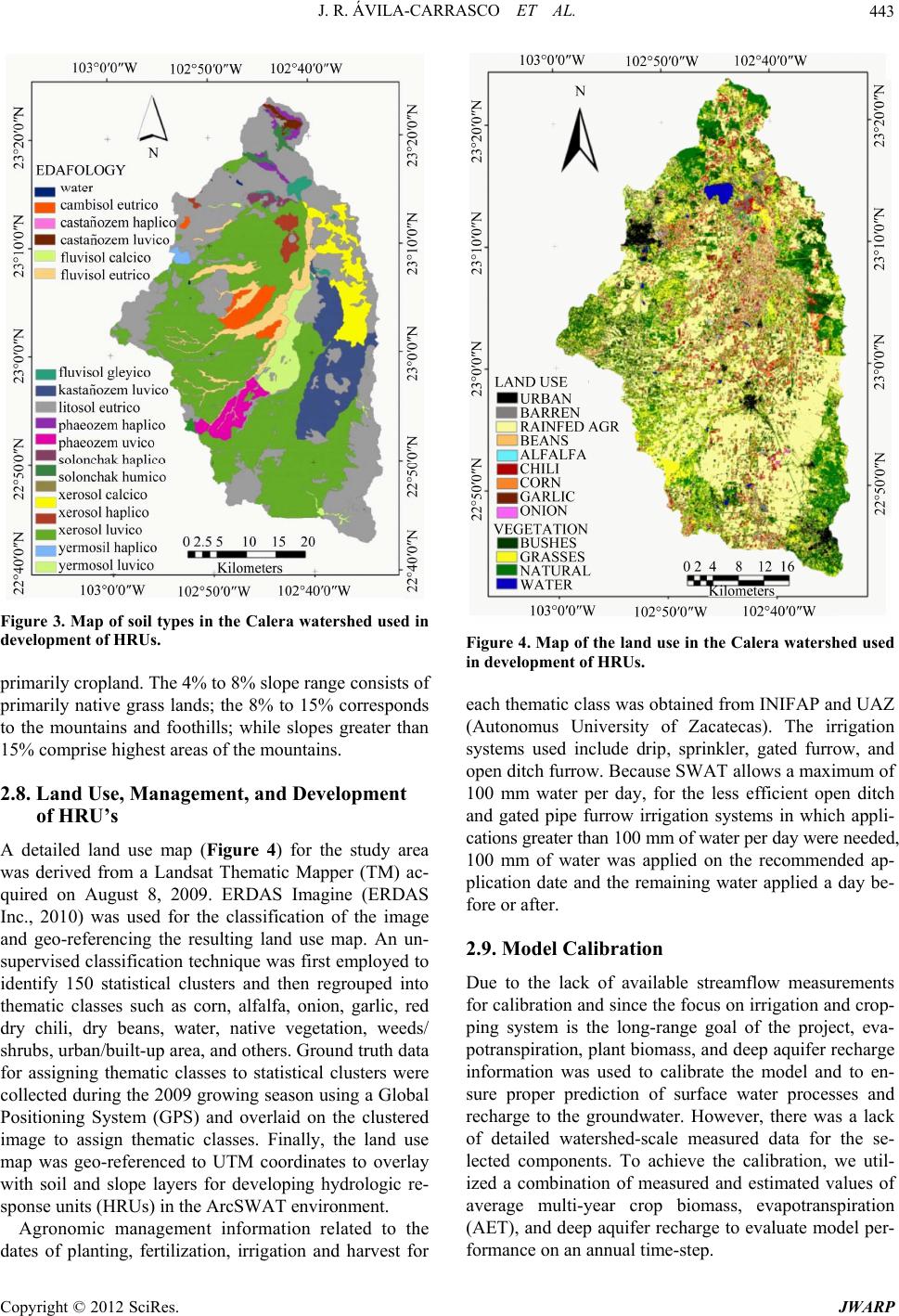 J. R. ÁVILA-CARRASCO ET AL. 443 Figure 3. Map of soil types in the Calera watershed used in development of HRUs. primarily cropland. The 4% to 8% slope range consists of primarily native grass lands; the 8% to 15% corresponds to the mountains and foothills; while slopes greater than 15% comprise highest areas of the mountains. 2.8. Land Use, Management, and Development of HRU’s A detailed land use map (Figure 4) for the study area was derived from a Landsat Thematic Mapper (TM) ac- quired on August 8, 2009. ERDAS Imagine (ERDAS Inc., 2010) was used for the classification of the image and geo-referencing the resulting land use map. An un- supervised classification technique was first employed to identify 150 statistical clusters and then regrouped into thematic classes such as corn, alfalfa, onion, garlic, red dry chili, dry beans, water, native vegetation, weeds/ shrubs, urban/built-up area, and others. Ground truth data for assigning thematic classes to statistical clusters were collected during the 2009 growing season using a Global Positioning System (GPS) and overlaid on the clustered image to assign thematic classes. Finally, the land use map was geo-referenced to UTM coordinates to overlay with soil and slope layers for developing hydrologic re- sponse units (HRUs) in the ArcSWAT environment. Agronomic management information related to the dates of planting, fertilization, irrigation and harvest for Figure 4. Map of the land use in the Calera watershed used in development of HRUs. each thematic class was obtained from INIFAP and UAZ (Autonomus University of Zacatecas). The irrigation systems used include drip, sprinkler, gated furrow, and open ditch furrow. Because SWAT allows a maximum of 100 mm water per day, for the less efficient open ditch and gated pipe furrow irrigation systems in which appli- cations greater than 100 mm of water per day were needed, 100 mm of water was applied on the recommended ap- plication date and the remaining water applied a day be- fore or after. 2.9. Model Calibration Due to the lack of available streamflow measurements for calibration and since the focus on irrigation and crop- ping system is the long-range goal of the project, eva- potranspiration, plant biomass, and deep aquifer recharge information was used to calibrate the model and to en- sure proper prediction of surface water processes and recharge to the groundwater. However, there was a lack of detailed watershed-scale measured data for the se- lected components. To achieve the calibration, we util- ized a combination of measured and estimated values of average multi-year crop biomass, evapotranspiration (AET), and deep aquifer recharge to evaluate model per- formance on an annual time-step. Copyright © 2012 SciRes. JWARP 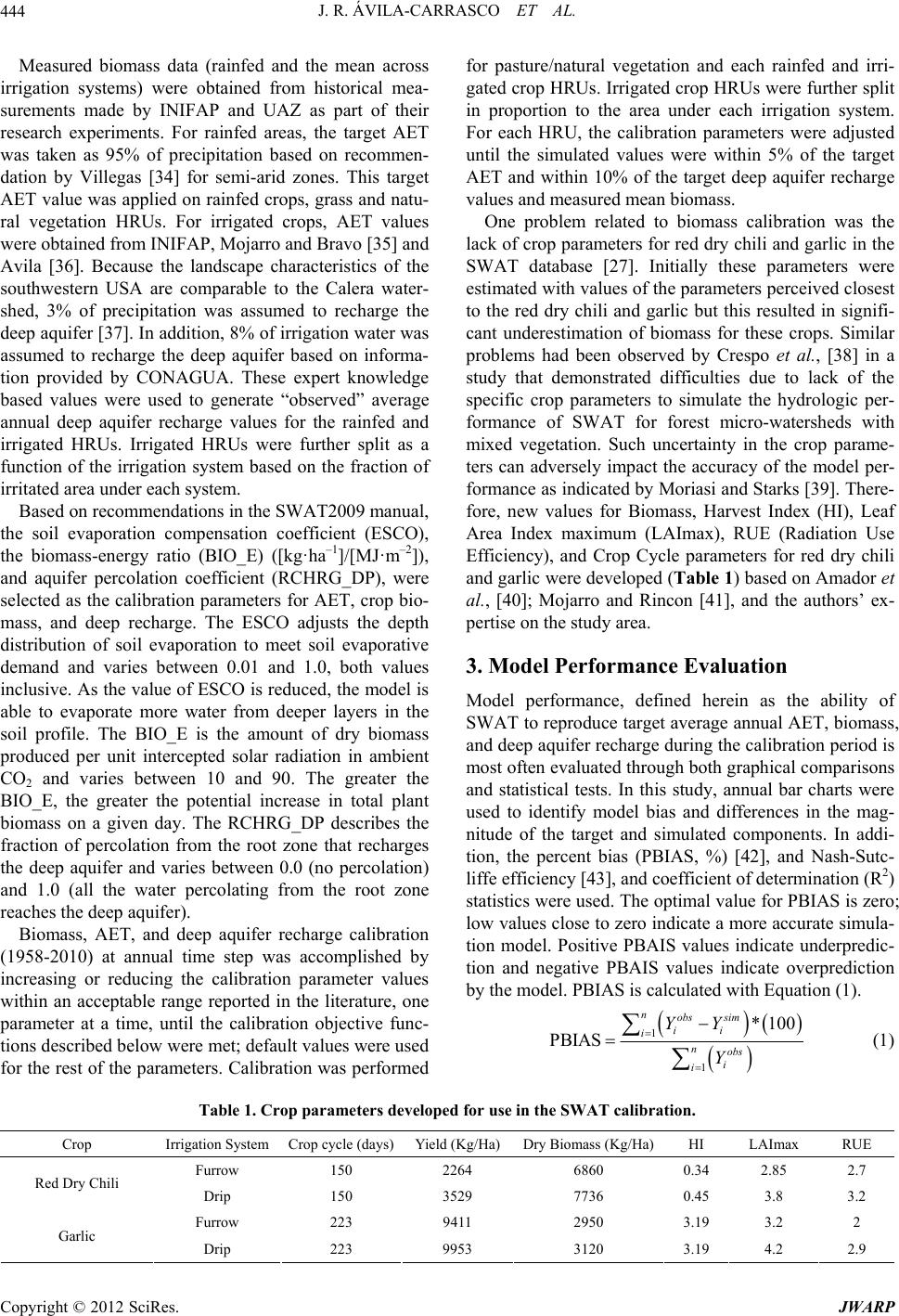 J. R. ÁVILA-CARRASCO ET AL. Copyright © 2012 SciRes. JWARP 444 Measured biomass data (rainfed and the mean across irrigation systems) were obtained from historical mea- surements made by INIFAP and UAZ as part of their research experiments. For rainfed areas, the target AET was taken as 95% of precipitation based on recommen- dation by Villegas [34] for semi-arid zones. This target AET value was applied on rainfed crops, grass and natu- ral vegetation HRUs. For irrigated crops, AET values were obtained from INIFAP, Mojarro and Bravo [35] and Avila [36]. Because the landscape characteristics of the southwestern USA are comparable to the Calera water- shed, 3% of precipitation was assumed to recharge the deep aquifer [37]. In addition, 8% of irrigation water was assumed to recharge the deep aquifer based on informa- tion provided by CONAGUA. These expert knowledge based values were used to generate “observed” average annual deep aquifer recharge values for the rainfed and irrigated HRUs. Irrigated HRUs were further split as a function of the irrigation system based on the fraction of irritated area under each system. Based on recommendations in the SWAT2009 manual, the soil evaporation compensation coefficient (ESCO), the biomass-energy ratio (BIO_E) ([kg·ha–1]/[MJ·m–2]), and aquifer percolation coefficient (RCHRG_DP), were selected as the calibration parameters for AET, crop bio- mass, and deep recharge. The ESCO adjusts the depth distribution of soil evaporation to meet soil evaporative demand and varies between 0.01 and 1.0, both values inclusive. As the value of ESCO is reduced, the model is able to evaporate more water from deeper layers in the soil profile. The BIO_E is the amount of dry biomass produced per unit intercepted solar radiation in ambient CO2 and varies between 10 and 90. The greater the BIO_E, the greater the potential increase in total plant biomass on a given day. The RCHRG_DP describes the fraction of percolation from the root zone that recharges the deep aquifer and varies between 0.0 (no percolation) and 1.0 (all the water percolating from the root zone reaches the deep aquifer). Biomass, AET, and deep aquifer recharge calibration (1958-2010) at annual time step was accomplished by increasing or reducing the calibration parameter values within an acceptable range reported in the literature, one parameter at a time, until the calibration objective func- tions described below were met; default values were used for the rest of the parameters. Calibration was performed for pasture/natural vegetation and each rainfed and irri- gated crop HRUs. Irrigated crop HRUs were further split in proportion to the area under each irrigation system. For each HRU, the calibration parameters were adjusted until the simulated values were within 5% of the target AET and within 10% of the target deep aquifer recharge values and measured mean biomass. One problem related to biomass calibration was the lack of crop parameters for red dry chili and garlic in the SWAT database [27]. Initially these parameters were estimated with values of the parameters perceived closest to the red dry chili and garlic but this resulted in signifi- cant underestimation of biomass for these crops. Similar problems had been observed by Crespo et al., [38] in a study that demonstrated difficulties due to lack of the specific crop parameters to simulate the hydrologic per- formance of SWAT for forest micro-watersheds with mixed vegetation. Such uncertainty in the crop parame- ters can adversely impact the accuracy of the model per- formance as indicated by Moriasi and Starks [39]. There- fore, new values for Biomass, Harvest Index (HI), Leaf Area Index maximum (LAImax), RUE (Radiation Use Efficiency), and Crop Cycle parameters for red dry chili and garlic were developed (Table 1) based on Amador et al., [40]; Mojarro and Rincon [41], and the authors’ ex- pertise on the study area. 3. Model Performance Evaluation Model performance, defined herein as the ability of SWAT to reproduce target average annual AET, biomass, and deep aquifer recharge during the calibration period is most often evaluated through both graphical comparisons and statistical tests. In this study, annual bar charts were used to identify model bias and differences in the mag- nitude of the target and simulated components. In addi- tion, the percent bias (PBIAS, %) [42], and Nash-Sutc- liffe efficiency [43], and coefficient of determination (R2) statistics were used. The optimal value for PBIAS is zero; low values close to zero indicate a more accurate simula- tion model. Positive PBAIS values indicate underpredic- tion and negative PBAIS values indicate overprediction by the model. PBIAS is calculated with Equation (1). 1 1 *100 PBIAS nobs sim ii i nobs i i YY Y (1) Table 1. Crop parameters developed for use in the SWAT calibration. Crop Irrigation System Crop cycle (days)Yield (Kg/Ha)Dry Biomass (Kg/Ha)HI LAImax RUE Furrow 150 2264 6860 0.34 2.85 2.7 Red Dry Chili Drip 150 3529 7736 0.45 3.8 3.2 Furrow 223 9411 2950 3.19 3.2 2 Garlic Drip 223 9953 3120 3.19 4.2 2.9 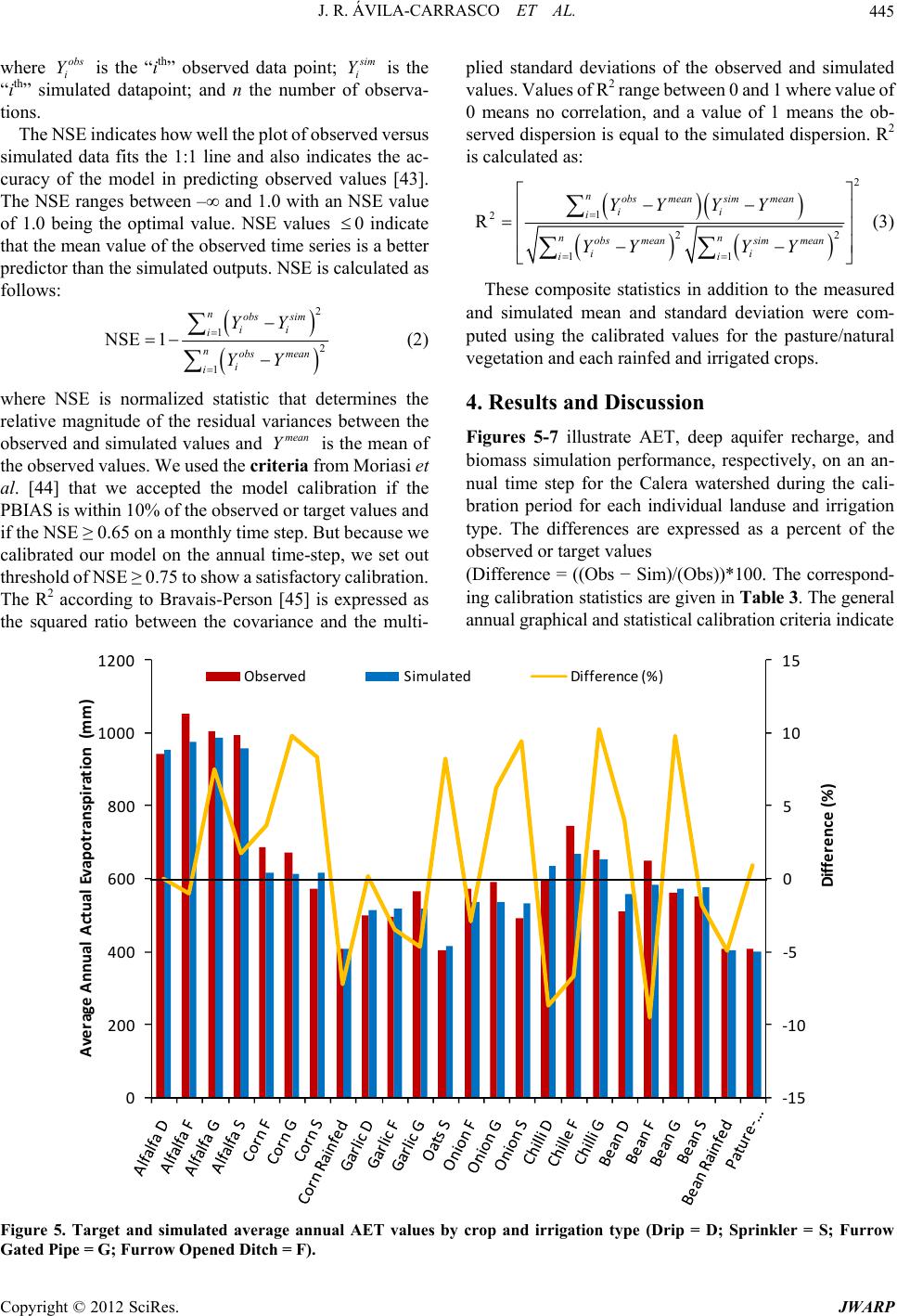 J. R. ÁVILA-CARRASCO ET AL. 445 where is the “ith” observed data point; obs i Y im i Y is the “ith” simulated datapoint; and n the number of observa- tions. The NSE indicates how well the plot of observed versus simulated data fits the 1:1 line and also indicates the ac- curacy of the model in predicting observed values [43]. The NSE ranges between –∞ and 1.0 with an NSE value of 1.0 being the optimal value. NSE values 0 indicate that the mean value of the observed time series is a better predictor than the simulated outputs. NSE is calculated as follows: 2 1 2 1 NSE 1 nobs sim ii i nobs mean i i YY YY (2) where NSE is normalized statistic that determines the relative magnitude of the residual variances between the observed and simulated values and is the mean of the observed values. We used the criteria from Moriasi et al. [44] that we accepted the model calibration if the PBIAS is within 10% of the observed or target values and if the NSE ≥ 0.65 on a monthly time step. But because we calibrated our model on the annual time-step, we set out threshold of NSE ≥ 0.75 to show a satisfactory calibration. mean Y The R2 according to Bravais-Person [45] is expressed as the squared ratio between the covariance and the multi- plied standard deviations of the observed and simulated values. Values of R2 range between 0 and 1 where value of 0 means no correlation, and a value of 1 means the ob- served dispersion is equal to the simulated dispersion. R2 is calculated as: 2 1 2 22 11 R nobs mean simmean ii i nn obs meansim mean ii ii YY YY YY YY (3) These composite statistics in addition to the measured and simulated mean and standard deviation were com- puted using the calibrated values for the pasture/natural vegetation and each rainfed and irrigated crops. 4. Results and Discussion Figures 5-7 illustrate AET, deep aquifer recharge, and biomass simulation performance, respectively, on an an- nual time step for the Calera watershed during the cali- bration period for each individual landuse and irrigation type. The differences are expressed as a percent of the observed or target values (Difference = ((Obs − Sim)/(Obs))*100. The correspond- ing calibration statistics are given in Table 3. The general annual graphical and statistical calibration criteria indicate -15 -10 -5 0 5 10 15 0 200 400 600 800 1000 1200 Difference (%) Average Annual Actual Evapotranspiration (mm) Observed Simulated Difference (%) Figure 5. Target and simulated average annual AET values by crop and irrigation type (Drip = D; Sprinkler = S; Furrow Gated Pipe = G; Furrow Opened Ditch = F). Copyright © 2012 SciRes. JWARP 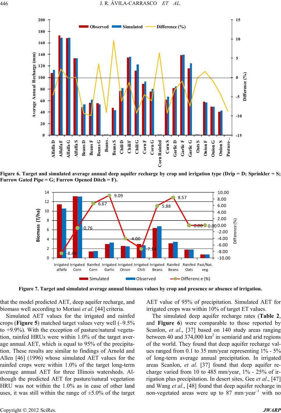 J. R. ÁVILA-CARRASCO ET AL. 446 -15 -10 -5 0 5 10 15 0 20 40 60 80 100 120 140 160 180 200 Alfal fa D Al fal fa F Al fal fa G Alfal fa S Beans D Beans F Beans Beans Beans S Chili D Chi li F Chili G Cor n F Corn G Cor n Rai nfe d Corn S Garlic D Garlic F Garlic G Oats S Onion F Onion G Onion S Pasture- Difference (%) Average Annual Recharge (mm) Observed Simulated Difference (%) Figure 6. Target and simulated average annua l deep aquifer recharge by crop and irrigation type (Drip = D; Sprinkler = S; Furrow Gated Pipe = G; Furrow Opened Ditch = F). -8.49 -0.76 6.67 9.09 -4.00 -7.14 5.88 8.57 0.00 0.00 -10.00 -8.00 -6.00 -4.00 -2.00 0.00 2.00 4.00 6.00 8.00 10.00 0 2 4 6 8 10 12 14 Irrigated alfalfa Irrigated Corn Rainfed Corn Irrigated Garlic Irrigated Onion Irrigated Chili Irrigated Beans Rainfed Be ans Rainfed Oats Past/Nat. ve g Biomass (T/ha) Simulated Observed Differenc e (%) Difference (%) Figure 7. Target and simulated average annual bioma ss values by crop and presence or absence of irrigation. that the model predicted AET, deep aquifer recharge, and biomass well according to Moriasi et al. [44] criteria. Simulated AET values for the irrigated and rainfed crops (Figure 5) matched target values very well (–9.5% to +9.9%). With the exception of pasture/natural vegeta- tion, rainfed HRUs were within 1.0% of the target aver- age annual AET, which is equal to 95% of the precipita- tion. These results are similar to findings of Arnold and Allen [46] (1996) whose simulated AET values for the rainfed crops were within 1.0% of the target long-term average annual AET for three Illinois watersheds. Al- though the predicted AET for pasture/natural vegetation HRU was not within the 1.0% as in case of other land uses, it was still within the range of ±5.0% of the target AET value of 95% of precipitation. Simulated AET for irrigated crops was within 10% of target ET values. The simulated deep aquifer recharge rates (Table 2, and Figure 6) were comparable to those reported by Scanlon, et al., [37] based on 140 study areas ranging between 40 and 374,000 km2 in semiarid and arid regions of the world. They found that deep aquifer recharge val- ues ranged from 0.1 to 35 mm/year representing 1% - 5% of long-term average annual precipitation. In irrigated areas Scanlon, et al. [37] found that deep aquifer re- charge varied from 10 to 485 mm/year, 1% - 25% of ir- rigation plus precipitation. In desert sites, Gee et al., [47] and Wang et al., [48] found that deep aquifer recharge in non-vegetated areas were up to 87 mm·year–1 with no Copyright © 2012 SciRes. JWARP 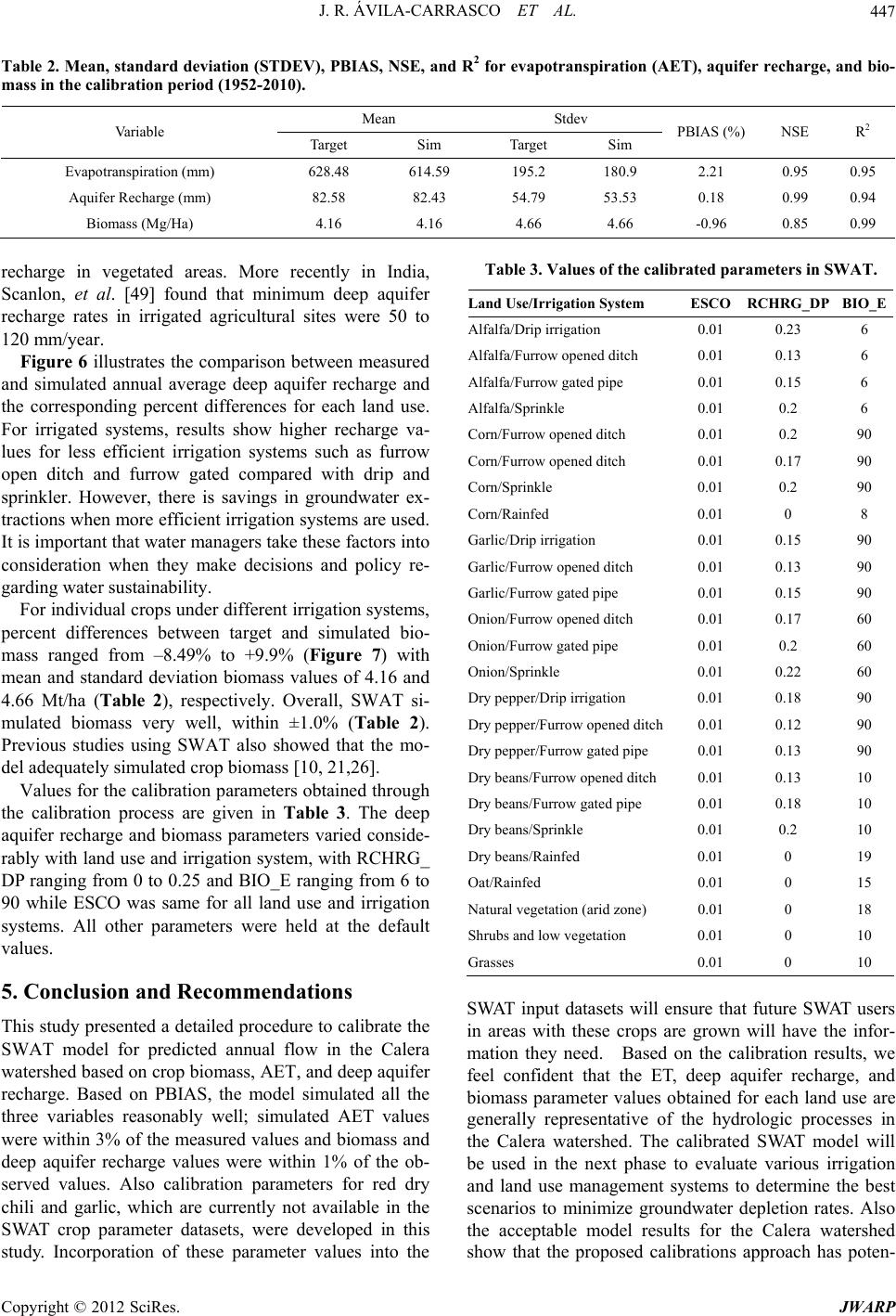 J. R. ÁVILA-CARRASCO ET AL. 447 Table 2. Mean, standard deviation (STDEV), PBIAS, NSE, and R 2 for evapotranspiration (AET), aquifer recharge, and bio- mass in the calibration period (1952-2010). Mean Stdev Va ri ab le Target Sim Target Sim PBIAS (%) NSE R2 Evapotranspiration (mm) 628.48 614.59 195.2 180.9 2.21 0.95 0.95 Aquifer Recharge (mm) 82.58 82.43 54.79 53.53 0.18 0.99 0.94 Biomass (Mg/Ha) 4.16 4.16 4.66 4.66 -0.96 0.85 0.99 recharge in vegetated areas. More recently in India, Scanlon, et al. [49] found that minimum deep aquifer recharge rates in irrigated agricultural sites were 50 to 120 mm/year. Figure 6 illustrates the comparison between measured and simulated annual average deep aquifer recharge and the corresponding percent differences for each land use. For irrigated systems, results show higher recharge va- lues for less efficient irrigation systems such as furrow open ditch and furrow gated compared with drip and sprinkler. However, there is savings in groundwater ex- tractions when more efficient irrigation systems are used. It is important that water managers take these factors into consideration when they make decisions and policy re- garding water sustainability. For individual crops under different irrigation systems, percent differences between target and simulated bio- mass ranged from –8.49% to +9.9% (Figure 7) with mean and standard deviation biomass values of 4.16 and 4.66 Mt/ha (Table 2), respectively. Overall, SWAT si- mulated biomass very well, within ±1.0% (Table 2). Previous studies using SWAT also showed that the mo- del adequately simulated crop biomass [10, 21,26]. Values for the calibration parameters obtained through the calibration process are given in Table 3. The deep aquifer recharge and biomass parameters varied conside- rably with land use and irrigation system, with RCHRG_ DP ranging from 0 to 0.25 and BIO_E ranging from 6 to 90 while ESCO was same for all land use and irrigation systems. All other parameters were held at the default values. 5. Conclusion and Recommendations This study presented a detailed procedure to calibrate the SWAT model for predicted annual flow in the Calera watershed based on crop biomass, AET, and deep aquifer recharge. Based on PBIAS, the model simulated all the three variables reasonably well; simulated AET values were within 3% of the measured values and biomass and deep aquifer recharge values were within 1% of the ob- served values. Also calibration parameters for red dry chili and garlic, which are currently not available in the SWAT crop parameter datasets, were developed in this study. Incorporation of these parameter values into the Table 3. Values of the calibrated parameters in SWAT. Land Use/Irrigation System ESCO RCHRG_DP BIO_E Alfalfa/Drip irrigation 0.01 0.23 6 Alfalfa/Furrow opened ditch 0.01 0.13 6 Alfalfa/Furrow gated pipe 0.01 0.15 6 Alfalfa/Sprinkle 0.01 0.2 6 Corn/Furrow opened ditch 0.01 0.2 90 Corn/Furrow opened ditch 0.01 0.17 90 Corn/Sprinkle 0.01 0.2 90 Corn/Rainfed 0.01 0 8 Garlic/Drip irrigation 0.01 0.15 90 Garlic/Furrow opened ditch 0.01 0.13 90 Garlic/Furrow gated pipe 0.01 0.15 90 Onion/Furrow opened ditch 0.01 0.17 60 Onion/Furrow gated pipe 0.01 0.2 60 Onion/Sprinkle 0.01 0.22 60 Dry pepper/Drip irrigation 0.01 0.18 90 Dry pepper/Furrow opened ditch 0.01 0.12 90 Dry pepper/Furrow gated pipe 0.01 0.13 90 Dry beans/Furrow opened ditch 0.01 0.13 10 Dry beans/Furrow gated pipe 0.01 0.18 10 Dry beans/Sprinkle 0.01 0.2 10 Dry beans/Rainfed 0.01 0 19 Oat/Rainfed 0.01 0 15 Natural vegetation (arid zone) 0.01 0 18 Shrubs and low vegetation 0.01 0 10 Grasses 0.01 0 10 SWAT input datasets will ensure that future SWAT users in areas with these crops are grown will have the infor- mation they need. Based on the calibration results, we feel confident that the ET, deep aquifer recharge, and biomass parameter values obtained for each land use are generally representative of the hydrologic processes in the Calera watershed. The calibrated SWAT model will be used in the next phase to evaluate various irrigation and land use management systems to determine the best scenarios to minimize groundwater depletion rates. Also the acceptable model results for the Calera watershed show that the proposed calibrations approach has poten- Copyright © 2012 SciRes. JWARP 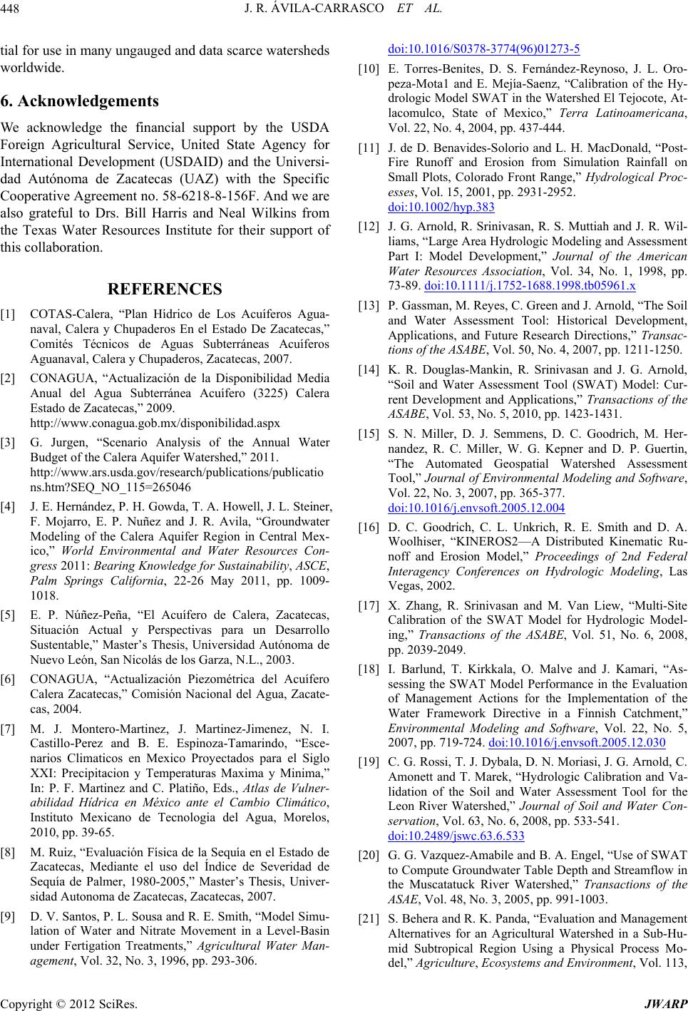 J. R. ÁVILA-CARRASCO ET AL. 448 tial for use in many ungauged and data scarce watersheds worldwide. 6. Acknowledgements We acknowledge the financial support by the USDA Foreign Agricultural Service, United State Agency for International Development (USDAID) and the Universi- dad Autónoma de Zacatecas (UAZ) with the Specific Cooperative Agreement no. 58-6218-8-156F. And we are also grateful to Drs. Bill Harris and Neal Wilkins from the Texas Water Resources Institute for their support of this collaboration. REFERENCES [1] COTAS-Calera, “Plan Hídrico de Los Acuíferos Agua- naval, Calera y Chupaderos En el Estado De Zacatecas,” Comités Técnicos de Aguas Subterráneas Acuíferos Aguanaval, Calera y Chupaderos, Zacatecas, 2007. [2] CONAGUA, “Actualización de la Disponibilidad Media Anual del Agua Subterránea Acuífero (3225) Calera Estado de Zacatecas,” 2009. http://www.conagua.gob.mx/disponibilidad.aspx [3] G. Jurgen, “Scenario Analysis of the Annual Water Budget of the Calera Aquifer Watershed,” 2011. http://www.ars.usda.gov/research/publications/publicatio ns.htm?SEQ_NO_115=265046 [4] J. E. Hernández, P. H. Gowda, T. A. Howell, J. L. Steiner, F. Mojarro, E. P. Nuñez and J. R. Avila, “Groundwater Modeling of the Calera Aquifer Region in Central Mex- ico,” World Environmental and Water Resources Con- gress 2011: Bearing Knowledge for Sustainability, ASCE, Palm Springs California, 22-26 May 2011, pp. 1009- 1018. [5] E. P. Núñez-Peña, “El Acuífero de Calera, Zacatecas, Situación Actual y Perspectivas para un Desarrollo Sustentable,” Master’s Thesis, Universidad Autónoma de Nuevo León, San Nicolás de los Garza, N.L., 2003. [6] CONAGUA, “Actualización Piezométrica del Acuífero Calera Zacatecas,” Comisión Nacional del Agua, Zacate- cas, 2004. [7] M. J. Montero-Martinez, J. Martinez-Jimenez, N. I. Castillo-Perez and B. E. Espinoza-Tamarindo, “Esce- narios Climaticos en Mexico Proyectados para el Siglo XXI: Precipitacion y Temperaturas Maxima y Minima,” In: P. F. Martinez and C. Platiño, Eds., Atlas de Vulner- abilidad Hídrica en México ante el Cambio Climático, Instituto Mexicano de Tecnologia del Agua, Morelos, 2010, pp. 39-65. [8] M. Ruiz, “Evaluación Física de la Sequía en el Estado de Zacatecas, Mediante el uso del Índice de Severidad de Sequía de Palmer, 1980-2005,” Master’s Thesis, Univer- sidad Autonoma de Zacatecas, Zacatecas, 2007. [9] D. V. Santos, P. L. Sousa and R. E. Smith, “Model Simu- lation of Water and Nitrate Movement in a Level-Basin under Fertigation Treatments,” Agricultural Water Man- agement, Vol. 32, No. 3, 1996, pp. 293-306. doi:10.1016/S0378-3774(96)01273-5 [10] E. Torres-Benites, D. S. Fernández-Reynoso, J. L. Oro- peza-Mota1 and E. Mejía-Saenz, “Calibration of the Hy- drologic Model SWAT in the Watershed El Tejocote, At- lacomulco, State of Mexico,” Terra Latinoamericana, Vol. 22, No. 4, 2004, pp. 437-444. [11] J. de D. Benavides-Solorio and L. H. MacDonald, “Post- Fire Runoff and Erosion from Simulation Rainfall on Small Plots, Colorado Front Range,” Hydrological Proc- esses, Vol. 15, 2001, pp. 2931-2952. doi:10.1002/hyp.383 [12] J. G. Arnold, R. Srinivasan, R. S. Muttiah and J. R. Wil- liams, “Large Area Hydrologic Modeling and Assessment Part I: Model Development,” Journal of the American Water Resources Association, Vol. 34, No. 1, 1998, pp. 73-89. doi:10.1111/j.1752-1688.1998.tb05961.x [13] P. Gassman, M. Reyes, C. Green and J. Arnold, “The Soil and Water Assessment Tool: Historical Development, Applications, and Future Research Directions,” Transac- tions of the ASABE, Vol. 50, No. 4, 2007, pp. 1211-1250. [14] K. R. Douglas-Mankin, R. Srinivasan and J. G. Arnold, “Soil and Water Assessment Tool (SWAT) Model: Cur- rent Development and Applications,” Transactions of the ASABE, Vol. 53, No. 5, 2010, pp. 1423-1431. [15] S. N. Miller, D. J. Semmens, D. C. Goodrich, M. Her- nandez, R. C. Miller, W. G. Kepner and D. P. Guertin, “The Automated Geospatial Watershed Assessment Tool,” Journal of Environmental Modeling and Software, Vol. 22, No. 3, 2007, pp. 365-377. doi:10.1016/j.envsoft.2005.12.004 [16] D. C. Goodrich, C. L. Unkrich, R. E. Smith and D. A. Woolhiser, “KINEROS2—A Distributed Kinematic Ru- noff and Erosion Model,” Proceedings of 2nd Federal Interagency Conferences on Hydrologic Modeling, Las Vegas, 2002. [17] X. Zhang, R. Srinivasan and M. Van Liew, “Multi-Site Calibration of the SWAT Model for Hydrologic Model- ing,” Transactions of the ASABE, Vol. 51, No. 6, 2008, pp. 2039-2049. [18] I. Barlund, T. Kirkkala, O. Malve and J. Kamari, “As- sessing the SWAT Model Performance in the Evaluation of Management Actions for the Implementation of the Water Framework Directive in a Finnish Catchment,” Environmental Modeling and Software, Vol. 22, No. 5, 2007, pp. 719-724. doi:10.1016/j.envsoft.2005.12.030 [19] C. G. Rossi, T. J. Dybala, D. N. Moriasi, J. G. Arnold, C. Amonett and T. Marek, “Hydrologic Calibration and Va- lidation of the Soil and Water Assessment Tool for the Leon River Watershed,” Journal of Soil and Water Con- servation, Vol. 63, No. 6, 2008, pp. 533-541. doi:10.2489/jswc.63.6.533 [20] G. G. Vazquez-Amabile and B. A. Engel, “Use of SWAT to Compute Groundwater Table Depth and Streamflow in the Muscatatuck River Watershed,” Transactions of the ASAE, Vol. 48, No. 3, 2005, pp. 991-1003. [21] S. Behera and R. K. Panda, “Evaluation and Management Alternatives for an Agricultural Watershed in a Sub-Hu- mid Subtropical Region Using a Physical Process Mo- del,” Agriculture, Ecosystems and Environment, Vol. 113, Copyright © 2012 SciRes. JWARP  J. R. ÁVILA-CARRASCO ET AL. 449 No. 1-4, 2006, pp. 62-72. doi:10.1016/j.agee.2005.08.032 [22] D. D. Bosch, J. M. Sheridan, H. L. Batten and J. G. Ar- nold, “Evaluation of the SWAT Model on a Coastal Plain Agricultural Watershed,” Transactions of the ASAE, Vol. 47, No. 5, 2004, pp. 1493-1506. [23] H. Cheng, W. Ouyang, F. Hao, X. Ren and S. Yang, “The Non-Point Source Pollution in Livestock-Breeding Areas of the Heihe River Basin in Yellow River,” Stochastic Environmental Research and Risk Assessment, Vol. 21, No. 3, 2007, pp. 213-221. [24] B. Du, J. G. Arnold, A. Saleh and D. B. Jaynes, “Devel- opment and Application of SWAT to Landscapes with Tiles and Potholes,” Transactions of the ASAE, Vol. 48, No. 3, 2005, pp. 1121-1133. [25] C. Qi and S. Grundwald, “GIS-Based Hydrologicic Mod- eling in Sandusky Watershed Using SWAT,” Transac- tions of the ASABE, Vol. 48, No. 1, 2005, pp. 169-180. [26] R. Srinivasan, X. Zhang and J. Arnold, “SWAT Un- gauged: Hydrological Budget and Crop Yield Predictions in the Upper Mississippi River Basin,” Transactions of the ASABE, Vol. 53, No. 5, 2010, pp. 1533-1546. [27] S. L. Neitsch, J. G. Arnold, J. R. Kiniry, R. Srinivasan and J. R. Willimas, “Soil and Water Assessment Tool In- put/Ouput File Documentation, Version 2009,” 2009. http://swatmodel.tamu.edu/media/19754/swat-io-2009.pdf [28] M. K. Kenneth, “National Engineering Handbook, Sec- tion 4 Hydrology, Chapter 15, Travel Time, Time of Concentration and Lag,” 1972. ftp://ftp.wcc.nrcs.usda.gov/wntsc/H%26H/NEHhydrology /ch21.pdf [29] J. L. Monteith, “Evaporation and the Environment in the State and Movement of Water in Living Organisms,” Proceedings of the Society for Experimental Biology, Symposium No. 19, Cambridge University Press, Cam- bridge, 1965, pp. 205-234. [30] L. Navarro, E. Nuñez, A. Cardona, J. Castro, E. Villal- pando and A. Bueno, “Analisis y Distribución de Elemen- tos Mayores en el Agua Subterránea del Acuífero de Calera, Zacatecas,” XV Congreso Nacional de Geoqui- mica INAGEQ Instituto Nacional de Geoquímica, Vol. 1, 2005. [31] E. Villalpando, E. Núñez, A. Cardona, J. Castro, L. Navarro and A. Bueno, “Distribución y Movilidad de Elementos traza en el Agua Subterránea de la Cuenca Hidrológica de Calera, Zacatecas,” Actas INAGEQ, 2005. [32] A. N. Sharpley and J. R. Williams, “EPIC. Erosion/Pro- ductivity Impact Calculator: 1. Model Documentation,” Technical Bulletin No. 1768, U.S. Department of Agri- culture (USDA), Madison, Wisconsin, 1990. [33] K. E. Saxton and W. J. Rawls, “Soil Water Characteristic Estimates by Texture and Organic Matter for Hydrologic Solutions,” Soil Science Society of America Journal, Vol. 70, No. 5, 2006, pp. 1569-1578. doi:10.2136/sssaj2005.0117 [34] J. C. Villegas, “Ecosystem Water Exchange and Parti- tioning of Evapotranspiration along Vegetation Gradients: Implications of Projected Dust-Bowl Climate in Ari- zona,” 2008. wsp.arizona.edu/sites/wsp.arizona.edu/files/uawater [35] D. F. Mojarro and L. A. Bravo, “Alternativas para Mejorar la Productividad del Agua de Riego: Caso Zaca- tecas, México,” Congreso Internacional de la Sociedad Mexicana de Horticultura, Zacatecas, 2007. [36] J. R. Avila-Carrasco, “Calibracion del Modelo Hidrolo- gico SWAT en la Cuenca Calera,” Master’s Thesis, Universidad Autonoma de Zacatecas, Zacatecas, 2011. [37] B. R. Scanlon, K. E. Keese, A. L. Flint, L. E. Flint, W. M. Edumunds and I. Simmers, “Global Synthesis of Ground- water Recharge in Semiarid and Arid Regions,” Hydrological Processes, Vol. 20, 2006, pp. 3335-3370. doi:10.1002/hyp.6335 [38] P. Crespo, C. Coello, V. Iñiguez, P. Cisneros, M. Ramírez, and J. Feyen, “Evaluación de SWAT2000 Como Herra- mienta Para el Análisis de Escenarios de Cambio de uso del suelo en Microcuencas de Montaña del sur del Ecuador,” 2008. http://www.secsuelo.org/simposios_xi_cons_mag.html [39] D. N. Moriasi and P. J. Starks, “Effects of the Resolution of Soil Dataset and Precipitation Dataset on SWAT2005 Streamflow Calibration Parameters and Simulation Ac- curacy,” Journal of Soil and Water Conservation, Vol. 65, No. 2 , 2010, pp. 63-78. [40] M. D. Amador-Ramirez, A. G. Bravo-Lozano, F. Mo- jarro-Davila and M. D. Alvarado-Nava, “Radiation Use Efficiency for Dry Chili Pepper Grown under Four Pro- duction Systems,” Second World Pepper Convention, Zacatecas, 2005, pp. 354-358. [41] D. F. Mojarro and F. Rincon, “Modelo de Crecimiento y Producción de Chile a Varios Ambientes: En Optimiza- cion del Sistema Producto Chile en la Region Norte- Centro de Mexico,” INIFAP, Zacatecas, 2002, pp. 44-55. [42] H. V. Gupta, S. Sorooshian and P. O. Yapo, “Status of Automatic Calibration for Hydrologic Models: Comparison with Multilevel Expert Calibration,” Journal of Hydrologic Engineering, Vol. 4, No. 2, 1999, pp. 135-143. doi:10.1061/(ASCE)1084-0699(1999)4:2(135) [43] J. E. Nash and R. M. Sutcliffe, “River Flow Forcasting through Conceptual Models: Part 1. A Discussion of Principles,” Journal Hydrology, Vol. 10, No. 3, 1970, pp. 282-290. doi:10.1016/0022-1694(70)90255-6 [44] D. N. Moriasi, J. G. Arnold, M. W. Van liew, R. L. Bingner, R. D. Harmel and T. L. Beith, “Model Evaluation Guidelines for Systematic Quantification of Accuracy in Watershed Simulations,” Transactions of the 5, No. 1, ASABE, Vol. 50, No. 3, 2007, pp. 885-900. [45] P. Krause, D. P. Boyle and F. Base, “Comparison of Different Efficiency Criteria for Hydrological Model Assessment,” Advances in Geosciencies, Vol. 2005, pp. 89-97. doi:10.5194/adgeo-5-89-2005 [46] J. G. Arnold and P. M. Allen, “Estimating Hydrologic Budgets for Three Illinois Waters Hydrology, Vol. 176, 1996, pp. 57-77 heds,” Journal of . doi:10.1016/0022-1694(95)02782-3 [47] G. W. Gee, P. J. Wierenga, B. J. Andraski, M. H. Young, Copyright © 2012 SciRes. JWARP  J. R. ÁVILA-CARRASCO ET AL. Copyright © 2012 SciRes. JWARP 450 ty of America Journal, Vol. M. J. Fayer and M. L. Rockhold, “Variations in Water Balance and Recharge Potential at Three Western Desert Sites,” Soil Science Socie No. 1, 1994, pp. 63-71. 58, doi:10.2136/sssaj1994.03615995005800010009x [48] X. P. Wang, R. Berndtsson, X. R. Li and E. S. Kang, “Water Balance Change for a Re-Vegetated Xerophyte Sciences Hydrologiques, Vol. 49, No. 2, 2004, pp. 283- 295. Shrub Area,” Hydrological Sciences Journal-Journal Des [49] B. R. Scanlon, M. Abhijit, J. Gates, R. C. Reedy and A. Sindha, “Groundwater Recharge in Natural Dune Systems and Agricultural Ecosystems in the Thar Desert Region, Rajasthan, India,” Hydrology Journal, Vol. 18, No. 4, 2010, pp. 959-972.
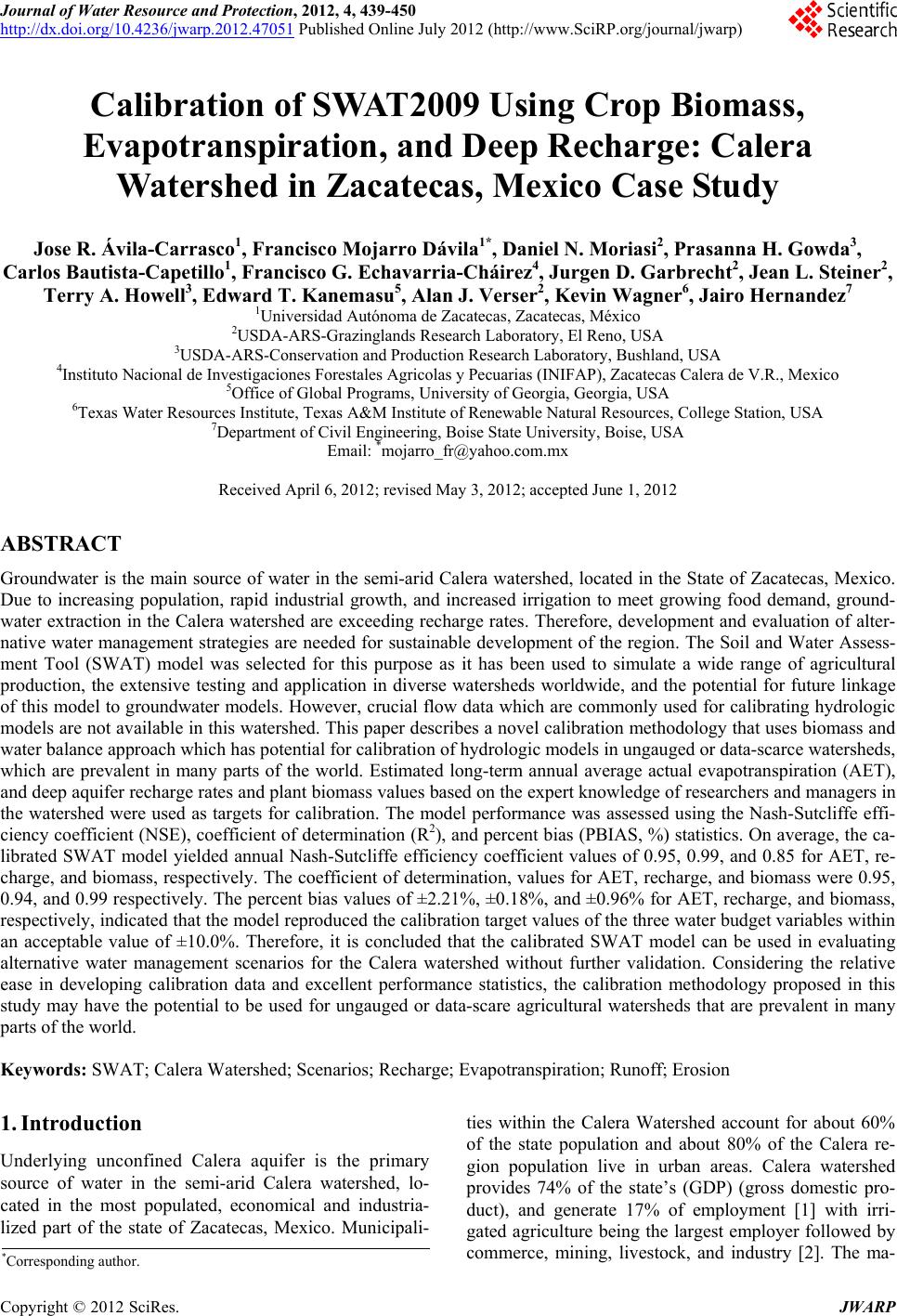
|