Paper Menu >>
Journal Menu >>
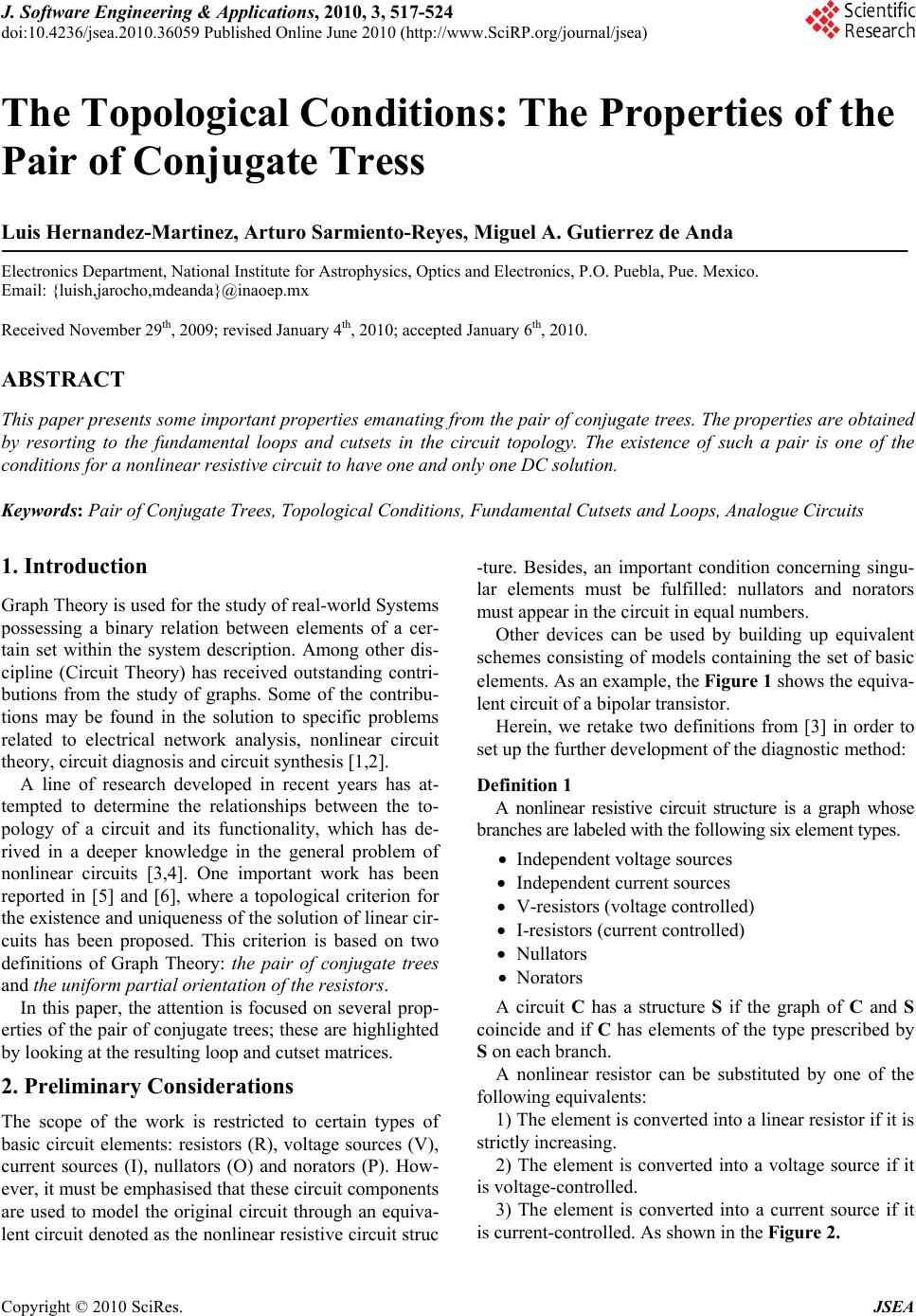 J. Software Engineering & Applications, 2010, 3, 517-524 doi:10.4236/jsea.2010.36059 Published Online June 2010 (http://www.SciRP.org/journal/jsea) Copyright © 2010 SciRes. JSEA The Topological Conditions: The Properties of the Pair of Conjugate Tress Luis Hernandez-Martinez, Arturo Sarmiento-Reyes, Miguel A. Gutierrez de Anda Electronics Department, National Institute for Astrophysics, Optics and Electronics, P.O. Puebla, Pue. Mexico. Email: {luish,jarocho,mdeanda}@inaoep.mx Received November 29th, 2009; revised January 4th, 2010; accepted January 6th, 2010. ABSTRACT This paper presents some important properties emanating from the pair of conjugate trees. The properties are obtained by resorting to the fundamental loops and cutsets in the circuit topology. The existence of such a pair is one of the conditions for a nonlinear resistive circuit to have one and only one DC solution. Keywords: Pair of Conjugate Trees, Topological Conditions, Fundamental Cutsets and Loops, Analogue Circuits 1. Introduction Graph Theory is used for the study of real-world Systems possessing a binary relation between elements of a cer- tain set within the system description. Among other dis- cipline (Circuit Theory) has received outstanding contri- butions from the study of graphs. Some of the contribu- tions may be found in the solution to specific problems related to electrical network analysis, nonlinear circuit theory, circuit diagnosis and circuit synthesis [1,2]. A line of research developed in recent years has at- tempted to determine the relationships between the to- pology of a circuit and its functionality, which has de- rived in a deeper knowledge in the general problem of nonlinear circuits [3,4]. One important work has been reported in [5] and [6], where a topological criterion for the existence and uniqueness of the solution of linear cir- cuits has been proposed. This criterion is based on two definitions of Graph Theory: the pair of conjugate trees and the uniform partial orientation of the resistors. In this paper, the attention is focused on several prop- erties of the pair of conjugate trees; these are highlighted by looking at the resulting loop and cutset matrices. 2. Preliminary Considerations The scope of the work is restricted to certain types of basic circuit elements: resistors (R), voltage sources (V), current sources (I), nullators (O) and norators (P). How- ever, it must be emphasised that these circuit components are used to model the original circuit through an equiva- lent circuit denoted as the nonlinear resistive circuit struc -ture. Besides, an important condition concerning singu- lar elements must be fulfilled: nullators and norators must appear in the circuit in equal numbers. Other devices can be used by building up equivalent schemes consisting of models containing the set of basic elements. As an example, the Figure 1 shows the equiva- lent circuit of a bipolar transistor. Herein, we retake two definitions from [3] in order to set up the further development of the diagnostic method: Definition 1 A nonlinear resistive circuit structure is a graph whose branches are labeled with the following six element types. Independent voltage sources Independent current sources V-resistors (voltage controlled) I-resistors (current controlled) Nullators Norators A circuit C has a structure S if the graph of C and S coincide and if C has elements of the type prescribed by S on each branch. A nonlinear resistor can be substituted by one of the following equivalents: 1) The element is converted into a linear resistor if it is strictly increasing. 2) The element is converted into a voltage source if it is voltage-controlled. 3) The element is converted into a current source if it is current-controlled. As shown in the Figure 2. 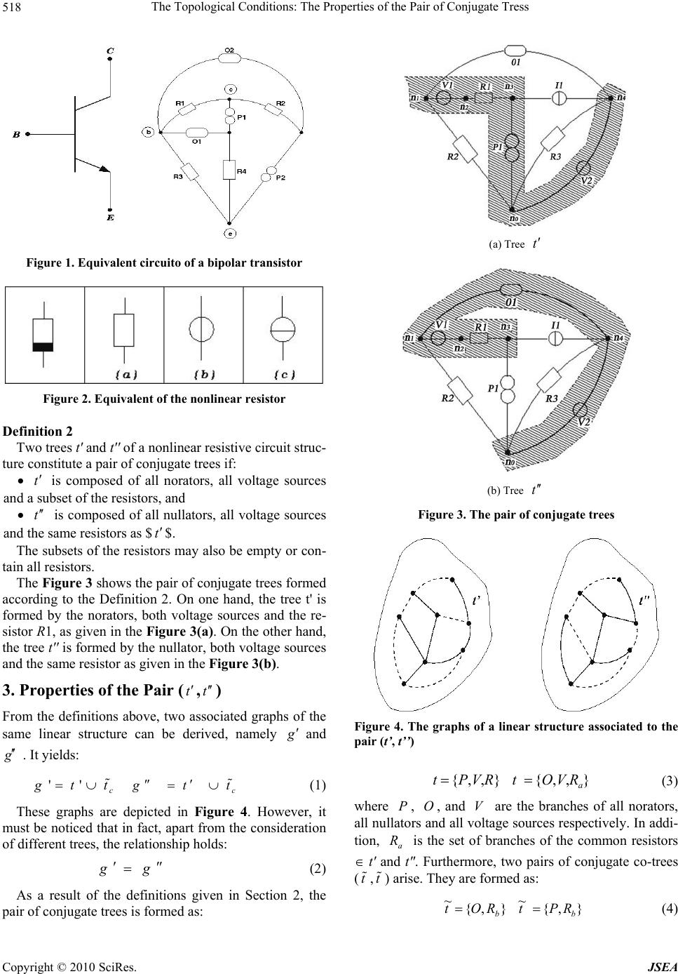 The Topological Conditions: The Properties of the Pair of Conjugate Tress 518 Figure 1. Equivalent circuito of a bipolar transistor Figure 2. Equivalent of the nonlinear resistor Definition 2 Two trees t' and t' ' of a nonlinear resistive circuit struc- ture constitute a pair of conjugate trees if: t is composed of all norators, all voltage sources and a subset of the resistors, and t is composed of all nullators, all voltage sources and the same resistors as $t$. The subsets of the resistors may also be empty or con- tain all resistors. The Figure 3 shows the pair of conjugate trees formed according to the Definition 2. On one hand, the tree t' is formed by the norators, both voltage sources and the re- sistor R1, as given in the Figure 3(a). On the other hand, the tree t'' is formed by the nullator, both voltage sources and the same resistor as given in the Figure 3(b). 3. Properties of the Pair (t,) t From the definitions above, two associated graphs of the same linear structure can be derived, namely g and . It yields: g ' ' c g tt c g tt (1) These graphs are depicted in Figure 4. However, it must be noticed that in fact, apart from the consideration of different trees, the relationship holds: g g (2) As a result of the definitions given in Section 2, the pair of conjugate trees is formed as: (a) Tree t (b) Tree t Figure 3. The pair of conjugate trees Figure 4. The graphs of a linear structure associated to the pair (t’, t’’) },,{RVP t (3) },,{ a RVO t where P , , and are the branches of all norators, all nullators and all voltage sources respectively. In addi- tion, is the set of branches of the common resistors t' and t". Furthermore, two pairs of conjugate co-trees (t,) arise. They are formed as: O V a R t },{ ~ b ROt } (4) ,{ ~ b RP t Copyright © 2010 SciRes. JSEA  The Topological Conditions: The Properties of the Pair of Conjugate Tress519 where is the set of branches of those resistors not in t' nor in t' '. It clearly results that the complete set of re- sistors , is formed by: b R R ba RRR (5) Some dimensions may be mentioned now: ptotal number of norators ototal number of nullators vtotal number of voltage sources atotal number of resistors a R btotal number of resistorsb R r total number of resistors R i.e. bar l total number of fundamental loops c total number of cutsets with the additional requirement of p = o. Besides, some variables must be defined: p unorators voltages o unullator voltages v uvoltage sources a uresistor voltages of a R b uresistor voltages of b R p inorators currents o inullators currents v icurrent sources a iresistor currents of a R b iresistor currents of b R 4. Properties Hereafter, the properties of the pair of conjugate trees (t , ) are obtained by resorting to the fundamental loops and fundamental cutsets of the associated graphs. Be- cause only one branch of the co-tree may be present in a fundamental loop, the structure of the fundamental loop matrix has the form: t ][][ LTLT ICCCC (6) where is the tree-part of the fundamental loop ma- trix, and LL is the co-tree part. Because only one branch of the tree may be present in a fundamental cutset, the structure of the fundamental cutset matrix has the form: T C C I LTLT DIDDD (7) where is the tree-part of the fundamental cutset matrix, and is the co-tree part. In the following, Kirchoff's Laws for both graphs are analyzed in order to determine the properties of the loops and cutsets. TT ID L D 4.1 KVL for g Since the co-tree branch present in a fundamental loop must belong either to O or , then the matrix in Equation (6) can have the form: Rb b o TI I CC where and are identity matrices of order o and b respectively. Two types of loops arise: o Ib I o l a loop in g having a link from O b l a loop in g having a link from b R Furthermore, can also be partitioned, which yields: T C b a babvbp oaovop I I C CC C C C C where every submatrix denoted as is a matrix of size xy C x y . Since op , is a square matrix. Moreover, the size of op C T C is )av() pb(o . KVL is given as: 0 u C The partitioning above allows us to establish KVL as: 0 b o a v p b o babvbp oaovop u u u u u I I CC C C C C (8) which is a system of loop equations in )( bo )( boavp branch voltages. For the nullors, 0 o U, then KVL can be re-written as: 0 b a v p b babvbp oaovop u u u u I C C C C C C (9) 4.2 KCL for g Since the tree branch present in a fundamental cutset must belong either to P or V or , then the matrix in Equation (7) can have the form: a R L a v p D I I I D where , and are identity matrices of order p Iv Ia I Copyright © 2010 SciRes. JSEA  The Topological Conditions: The Properties of the Pair of Conjugate Tress 520 p , v and respectively. Three types of cutsets arise: a p c a cutest in having a twig g from P v c a c a cutest in having a twig g from V a cutest in having a twig g from a R Furthermore, can also be partitioned, which yields: L D abao vbvo pbpo a v p D D D D D D I I I D where every submatrix denoted as is a matrix of size . Since , is a square matrix. Moreover, the size of is . KCL is given as: xy D )a xypo L D po D (vp )( bo oi D The partitioning above allows us to establish KCL as: 0 b o a v p ab vb pb ao vo pa a v p i i i i i D D D D D D I I I (10) which is a system of )( bvp cutset equations in branch currents. For the nullors, , then KCL can be re-written as: )ba (p o i ov 0 0 b a v p ab vb pb a v p T op C T bp C i i i i D D D I I I (11) Based on the orthogonality relationship: T TT DC where stands for the transpose of (see the Figure 5), the following equalities arise: T T DT D po D vo T ov DC av T oa DC pb D (12) vb T bv DC ab T ba DC In order to illustrate the properties of the work, con- sider the linear circuit given in Figure 6, the fundamental loop and cutset matrices are given by: P1 V 1 V2 R 1 O 1 R 2 R 3 l ' 1 1 1 1 1 1 C'= l' 2 1 1 1 1 l ' 3 1 1 P1 V1 V2 R 1 O 1 R 2 R 3 c'1 1 1 1 0 D'= c'2 1 1 1 0 c'3 1 1 0 1 c'4 1 1 1 0 Figure 5. Orthogonality in g Figure 6. Case of study where the columns have been labelled with the element names and the rows with the loop and cutsets respec- tively. The labels however, do not belong to the matrix. 4.3 KVL for g Since the co-tree branch present in a fundamental loop must belong either to P or , then the matrix in Equ- ation (6) can have the form: b R Copyright © 2010 SciRes. JSEA 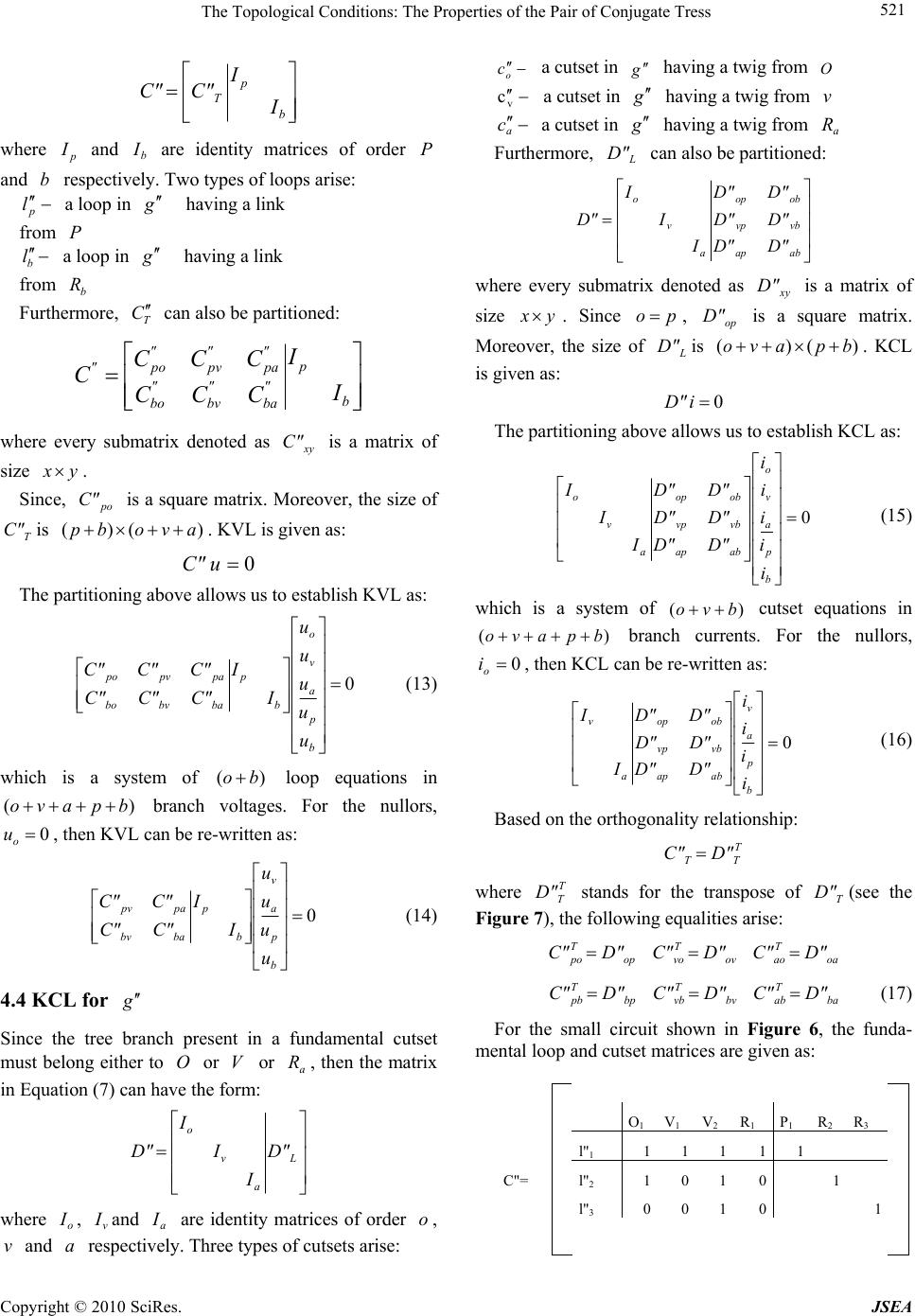 The Topological Conditions: The Properties of the Pair of Conjugate Tress521 b p TI I C"C" where and are identity matrices of order p Ib I P and respectively. Two types of loops arise: b p l a loop in having a link g from P b l a loop in having a link g from b R Furthermore, can also be partitioned: T C b p " ba " bv " bo " pa " pv " po " I I CCC CCC C where every submatrix denoted as is a matrix of size xy C" y x . Since, is a square matrix. Moreover, the size of is . KVL is given as: po C" )bp T C" )(( avo 0 uC" The partitioning above allows us to establish KVL as: 0 b p a v o b p babvbo papvpo u u u u u I I C"C"C" C"C"C" (13) which is a system of )( bo loop equations in branch voltages. For the nullors, , then KVL can be re-written as: )( bpavo 0 o u 0 b p a v b p babv papv u u u u I I C"C" C"C" (14) 4.4 KCL for g Since the tree branch present in a fundamental cutset must belong either to or V or , then the matrix in Equation (7) can have the form: Oa R L a v o D" I I I D" where , and are identity matrices of order , and a respectively. Three types of cutsets arise: o Iv Ia Io v o c a cutset in g having a twig from O v c a cutset in g having a twig from v a c a cutset in g having a twig from a R Furthermore, can also be partitioned: L D" abap vbvp obop a v o D"D" D"D" D"D" I I I D" where every submatrix denoted as is a matrix of size xy D" y x . Since po , is a square matrix. Moreover, the size of is op D" (o L D" )( bp)av . KCL is given as: 0iD" The partitioning above allows us to establish KCL as: 0 b p a v o abap vbvp obop a v o i i i i i D"D" D"D" D"D" I I I (15) which is a system of cutset equations in branch currents. For the nullors, )( bvo )( bpavo 0 o i, then KCL can be re-written as: 0 b p a v abap vbvp obop a v i i i i D"D" D"D" D"D" I I (16) Based on the orthogonality relationship: T TTD"C" where stands for the transpose of (see the Figure 7), the following equalities arise: T T D" T D" op T po D"C" ov T vo D"C" oa T ao D"C" bp T pb D"C" (17) bv T vb D"C" ba T ab D"C" For the small circuit shown in Figure 6, the funda- mental loop and cutset matrices are given as: O1V1 V 2 R 1 P 1 R 2R3 l"1 1 1 1 1 1 C"= l"2 10 1 0 1 l"3 00 1 0 1 Copyright © 2010 SciRes. JSEA 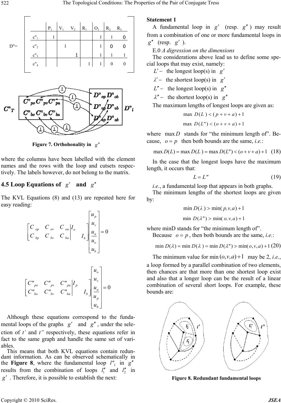 The Topological Conditions: The Properties of the Pair of Conjugate Tress 522 P1 V 1 V 2 R 1 O 1 R 2 R 3 c"1 1 1 10 D"= c"2 1 1 0 0 c"3 1 1 11 c"4 1 1 00 Figure 7. Orthohonality in g where the columns have been labelled with the element names and the rows with the loop and cutsets respec- tively. The labels however, do not belong to the matrix. 4.5 Loop Equations of and g g The KVL Equations (8) and (13) are repeated here for easy reading: 0 b o a v p b o babvbp oaovop u u u u u I I C C C C C C 0 b p a v o b p babvbo papvpo u u u u u I I C"C"C" C"C"C" Although these equations correspond to the funda- mental loops of the graphs g and , under the sele- ction of t’ and t” respectively, these equations refer in fact to the same graph and handle the same set of vari- ables. g This means that both KVL equations contain redun- dant information. As can be observed schematically in the Figure 8, where the fundamental loop 1 l" in g results from the combination of loops 1 l and 2 l in . Therefore, it is possible to establish the next: g Statement 1 A fundamental loop in (resp. ) may result from a combination of one or more fundamental loops in gg g (resp. g ). E.0 A digression on the dimensions The considerations above lead us to define some spe- cial loops that may exist, namely: L the longest loop(s) in g λ the shortest loop(s) in g L the longest loop(s) in g the shortest loop(s) in g The maximum lengths of longest loops are given as: 1)() (max avpLD 1)()"(max avoLD where stands for “the minimum length of”. Be- cause, Dmax po then both bounds are the same, i.e.: 1)()"(max) (max)(max avoLDLDLD (18) In the case that the longest loops have the maximum length, it occurs that: L " L (19) i.e., a fundamental loop that appears in both graphs. The minimum lengths of the shortest loops are given by: 1)min() (minav,p,λD 1)min()"(min av,o,D where minD stands for “the minimum length of”. Because po , then both bounds are the same, i.e.: 1),,min()"(min) (min)(min avoDDD (20) The minimum value for min may be 2, i.e., a loop formed by a parallel combination of two elements, then chances are that more than one shortest loop exist and also that a longer loop can be the result of a linear combination of several short loops. For example, these bounds are: 1),,( avo Figure 8. Redundant fundamental loops Copyright © 2010 SciRes. JSEA 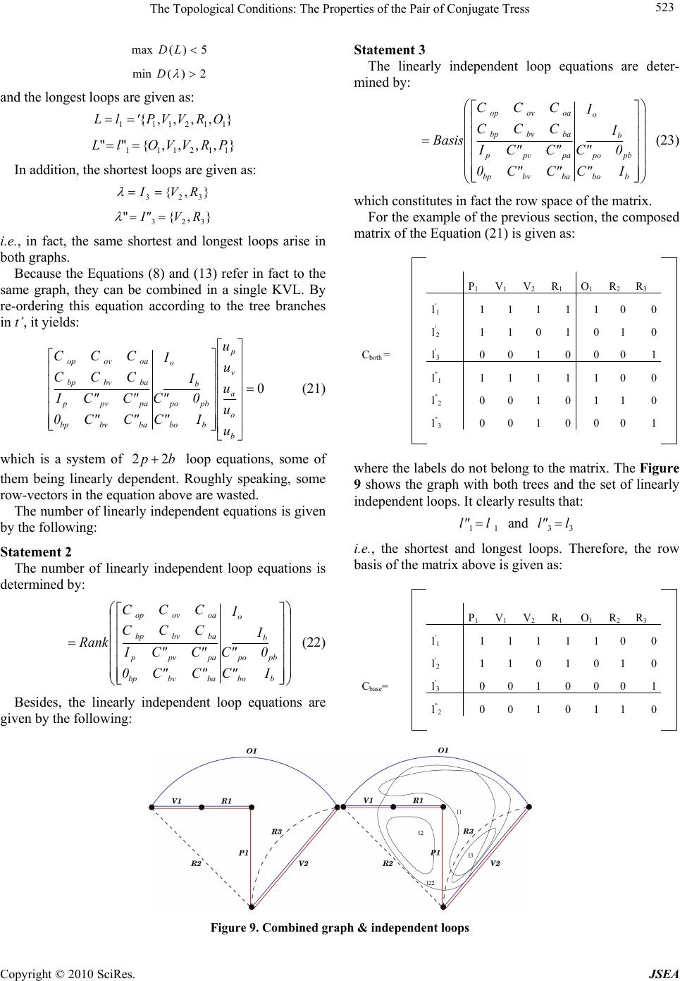 The Topological Conditions: The Properties of the Pair of Conjugate Tress Copyright © 2010 SciRes. JSEA 523 5)(max LD Statement 3 The linearly independent loop equations are deter- mined by: 2)(min D and the longest loops are given as: bbo pbpo b o babvbp papvp babvbp oaovop IC" 0C" I I C"C"0 C"C"I C C C C C C Basis (23) },,,,{ 112111ORVVPl L },,,,{"" 112111 PRVVOlL In addition, the shortest loops are given as: },{ 323 RVI which constitutes in fact the row space of the matrix. },{"323 RVI" For the example of the previous section, the composed matrix of the Equation (21) is given as: i.e., in fact, the same shortest and longest loops arise in both graphs. P1 V 1 V 2 R 1 O 1 R 2R3 l'1 11 1 1 1 00 l'2 11 0 1 0 10 Cboth = l'3 00 1 0 0 01 l"1 11 1 1 1 00 l"2 00 1 0 1 10 l"3 00 1 0 0 01 Because the Equations (8) and (13) refer in fact to the same graph, they can be combined in a single KVL. By re-ordering this equation according to the tree branches in t’, it yields: 0 b o a v p bbo pbpo b o babvbp papvp babvbp oaovop u u u u u IC" 0C" I I C"C"0 C"C"I C C C C C C (21) which is a system of loop equations, some of them being linearly dependent. Roughly speaking, some row-vectors in the equation above are wasted. bp 22 where the labels do not belong to the matrix. The Figure 9 shows the graph with both trees and the set of linearly independent loops. It clearly results that: The number of linearly independent equations is given by the following: 11 ll" and 33 ll" i.e., the shortest and longest loops. Therefore, the row basis of the matrix above is given as: Statement 2 The number of linearly independent loop equations is determined by: P1 V 1 V 2 R 1 O 1 R 2R3 l'1 11 1 1 1 00 l'2 11 0 1 0 10 Cbase= l'3 00 1 0 0 01 l"2 00 1 0 1 10 bbo pbpo b o babvbp papvp babvbp oaovop IC" 0C" I I C"C"0 C"C"I C C C C C C Rank (22) Besides, the linearly independent loop equations are given by the following: Figure 9. Combined graph & independent loops  The Topological Conditions: The Properties of the Pair of Conjugate Tress 524 5. Conclusions A set of properties of the pair of conjugate trees of within the graph emanating from nonlinear resistive circuits has been presented. This approach is obtained by lookinkg at the resulting loop and cutset matrices. REFERENCES [1] A. F. Schwarz, “Computer-Aided Design of Microelec- tronic Circuits and Systems,” Academic Press, Cambridge, Vol. 1, 1987. [2] J. Vlach and K. Singhal, “Computer Methods for Circuit Analysis and Design,” Van Nostrand Reinhold Company, New York, 1983. [3] M. Hasler, “Stability of Parasitic Dynamics at a dc- Operating Point: Topological Analysis,” Proceedings of the IEEE International Symposium on Circuits and Sys- tems, Singapore, 1991, pp. 770-773. [4] N. Tetsuo and C. Leon~O, “Topological Conditions for a Resistive Circuit Containing Negative Non-Linear Resis- tors to Have a Unique Solution,” International Journal on Circuit Theory and Applications, Vol. 15, Vol. 2, July 1987, pp. 193-210. [5] M. Fosseprez, M. Hasler and C. Schnetzler, “On the Num- ber of Solutions of Piecewise-Linear Resistive Circuits,” IEEE Transactions on Circuits and Systems, Vol. 18, No. 3, March 1989, pp. 393-402. [6] M. Fossèprez and M. Hasler, “Resistive Circuit Topolo- gies that Admit Several Solutions,” International Journal on Circuit Theory and Applications, Vol. 18, No. 6, Dece- mber 1990, pp. 625-638. Copyright © 2010 SciRes. JSEA |