Advances in Pure Mathematics, 2012, 2, 177-182
http://dx.doi.org/10.4236/apm.2012.23024 Published Online May 2012 (http://www.SciRP.org/journal/apm)
On Lorentzian α-Sasakian Manifolds
Subbegowda Lokesh, Venkatesha, Channabasappa Shantappa Bagewadi,
Kuntinamadu Thimmappa Pradeep Kumar
Department of P.G. Studies and Research in Mathematics, Kuvempu University, Shimoga, India
Received December 10, 2011; revised February 10, 2012; accepted February 18, 2012
ABSTRACT
The object of the present paper is to study Lorentzian α-Sasakian manifolds satisfying certain conditions on the W2-
curvature tensor.
Keywords: Lorentzian α-Sasakian Manifold; W2-Curvature Tensor; Einstein Manifold
1. Introduction
In 1970, Pokhariyal and Mishra [1] have introduced new
curvature tensor called W2-curvature tensor in a Rieman-
nian manifold and studied their properties. Further, Pok-
hariyal [2] has studied some properties of this curvature
tensor in a Sasakian manifold. Matsumoto, Ianus and
Mihai [3], Ahmet Yildiz and U. C. De [4] and Venkate-
sha, C. S. Bagewadi, and K. T. Pradeep Kumar [5], have
studied W2-curvature tensor in P-Sasakian, Kenmotsu
and Lorentzian para-Sasakian manifolds respectively.
In [6], S. Tanno classified connected almost contact
metric manifolds whose automorphism groups possess
the maximum dimension. For such a manifold, the sec-
tional curvature of a plane sections containing is a con-
stant, say c. He showed that they can be divided into
three classes:
1) Homogeneous normal contact Riemannian mani-
folds with c > 0;
2) Global Riemannian products of a line or a circle
with a Kaehler manifold of constant holomorphic sec-
tional curvature if c = 0 and;
3) A warped product space f if c > 0. It is
known that the manifolds of class (1) are characterized
by admitting a Sasakian structure.

In the Gray-Hervella classification of almost Hermi-
tian manifolds [7], there appears a class, W4, of Hermi-
tian manifolds which are closely related to locally con-
formal Kaehler manifolds [8]. An almost contact metric
structure on a manifold M is called a trans-Sasakian
structure [9] if the product manifold
M

CC

,,,
belongs to
the class W4. The class 65 ([10,11]) coincides with
the class of the trans-Sasakian structures of type (α, β). In
fact, in [11], local nature of the two subclasses, namely,
C5 and C6 structures of trans-Sasakian structures are
characterized completely.
We note that trans-Sasakian structures of type (0, 0),
(0, β) and (α, 0) are cosymplectic [12], β-Kenmotsu [13]
and α-Sasakian [13] respectively. In [14] it is proved that
trans-Sasakian structures are generalized quasi-Sasakian.
Thus, trans-Sasakian structures also provide a large class
of generalized quasi-Sasakian structures.
g
An almost contact metric structure 

,,
on M
is called a trans-Sasakian structure [9] if
M
JG
belongs to the class W4 [7], where J is the almost com-
plex structure on  defined by
M





,d, d,
J
Xfd tXfXd t  
for all vector fields X on M and smooth functions f on
, and G is the product metric on
M
M


. This
may be expressed by the condition [15]




 
 
,
,,
XYgXYYX
g
XYY X
 
 
 

for some smooth functions α and β on M, and we say that
the trans-Sasakian structure is of type (α, β).
A trans-Sasakian structure of type (α, β) is α-Sasakian
if β = 0 and α a nonzero constant [16]. If α = 1, then
α-Sasakian manifold is a Sasakian manifold.
2. Preliminaries
A differentiable manifold of dimension n is called Lor-
entzian α-Sasakian manifold if it admits a (1, 1)-tensor
field

, a contravariant vector field

, a covariant vec-
tor field

and Lorentzian metric g satisfy ([17-19])


1, 


2,I
(2.1)

 (2.2)






,, ,
g
XY gXYXY    (2.3)
C
opyright © 2012 SciRes. APM

S. LOKESH ET AL.
178



,,
g
XX  

0, 0,X   
(2.4)
(2.5)
for all ,.
X
YTM
Also a Lorentzian α-Sasakian manifold M is satisfying
[18]
 
,(b)),,(a XX
X
YgXY    
   
(2.6)
where denotes the operator of covariant differentia-
tion with respect to the Lorentzian metric g.

Further, on Lorentzian α-Sasakian manifold M the fol-
lowing relations hold:

 
2,,XZY

  
2
,,,RXY gXYYX   
,,RX YZgYZX g  
(2.7)
(2.8)




,X XY  
2
,RXY Y   (2.9)


 
2
RX X  

,,X  

2
,1,X 

2
1 ,nX Y   

(2.10)

SX n   (2.11)
,,SXY SXY   (2.12)
for all vector fields X, Y, Z where S is the Ricci tensor
and Q is the Ricci operator given by

,,.SXY gQXY
An Lorentzian α-Sasakian manifold M is said to be
Einstein if its Ricci tensor S is of the form


,,,SXY agXY

(2.13)
for any vector fields X and Y, where α is a function on M.
In [1], Pokhariyal and Mishra have defined the curva-
ture tensor W2, given by

2,, ,,, ,
1,,, ,,
–
1n
WXYUV RXYUV
gXUSYV gYUSXV





(2.14)
where S is a Ricci tensor of type (0, 2).
Consider in an Lorentzian α-Sasakian manifold satis-
fying W2 = 0 in (2.14), then we have


,, ,
11 ,,,,.
RXYUV
ngYUSXVgXUSYV  

 
,1,.SYVn gYV  
(2.15)
Putting X = U = in (2.15) then using (2.8) and (2.11),
we obtain
2 (2.16)
Thus M is an Einstein manifold.
Theorem 2.1. If on a Lorentzian α-Sasakian manifold
M, the condition W2 = 0 holds, then M is an Einstein
manifold.
Definition 2.1. An Lorentzian α-Sasakian manifold is
called W2-semisymmetric if it satisfies


2
,0,RXY W (2.17)



where

,RXY is to be considered as a derivation of
the tensor algebra at each point of the manifold for tan-
gent vectors X and Y.
In an Lorentzian α-Sasakian manifold the W2-curva-
ture tensor satisfies the condition


 
2,0.WXYZ
  (2.18)
3. Lorentzian α-Sasakian Manifolds
Satisfying


2
,0

PXY W
P

The pseudo projective curvature tensor is defined as
[20]




 
,
,
,,
,,.
1
PXY Z
aRX YZ
bSYZX SXZY
ra bgYZXgXZY
nn




 



 



Using (2.8) and (2.11), Equation (3.1) reduces to




 
2
,,
,1.
PYZhgYZ ZY
bSYZn ZY

 
 







where 2
1
ra
ha b
nn




 







.
Now consider in a Lorentzian α-Sasakian manifold


2
,0PXY W
.
This condition implies that









22
22
,, ,,
,,,, 0.
PXYW UVZWPXYUVZ
WUPXYVZWUVPXYZ





X
(3.3)
Put


in (3.3) and then taking the inner product
with

, we obtain

 


 





2
2
2
2
,,,
,,,
,, ,
,,,0.
gPYWUVZ
gWPYUVZ
gWUPYV Z
gWUVPYZ











(3.4)

Using (3.2) in (3.4), we obtain

S. LOKESH ET AL. 179
  
   
   
   
 

   
  
  
 

 
22
22
22
2
2
2
2
2
2
2
2
,,,
,,
,, ,
,,
1,
1(,
1,
1,
hgYWUVZ gYU
gYVWUZgYZ
YWUVZUW
VWUVZZW
bS YWUVZS YUW
SYVW UZSYZ
nYWUVZ
nUWYVZ
nVWUVZ
nZWUV
 
 
  
  


 
22
22
22
,
,,
,,
,,
,
,,
W VZ
W UV
YVZ
UVY
V Z
W UV



 
 






















0.Y





(3.5)
By using (2.18) in (3.5), we get
 


2
, 0.UVZ 

UZ
2
,, ,hgYW UVZbSYW

 (3.6)
Taking

 in (3.6) and using (2.14) and
(2.10), we have
 
,
11
SYV
n


 




2
2
,
,0.
bh
SQYV
n
hgV
b
Y







(3.7)
If b = 0, we get

2
1
1
hSYV
n



,,
0.gYV





,1,.n gYV

Then, either h = 0 (or)

2
SYV 
If b ≠ 0, then we get
 

,
1,.
hSYV
b
ngVY




2
2
,1S QYVn
h
b





(3.8)
Thus, we can state the following:
Theorem 3.2. If M is an Lorentzian α-Sasakian mani-
fold satisfying the condition


,0Y W

2
,0Y W
2
PX
 Then:
 If b = 0, then either h = 0 on M, or M is an Einstein
manifold;
 If b ≠ 0, then the Equation (3.8) holds on M.
4. Lorentzian α-Sasakian Manifold
Satisfying

ZX
The concircular curvature tensor Z is defined as [21]



,,
1
ZXYZ RXYZ
r
Using (2.8) and (2.11), Equation (4.1) reduces to
 
,, .
g
YZX
nn






g XZY


 
(4.1)
 
2
,,.
1
r
Z
YZgYZ ZY
nn
 

 





 (4.2)
Now consider in a Lorentzian α-Sasakian manifold


2
,0.ZXY W

This condition implies that









22
22
,, ,,
,,,, 0.
ZXYWUVZW ZXYUVZ
WUZXYVZWUVZXYZ





X
(4.3)
Put


in (4.3) and then taking the inner product
with

, we obtain







 


2
2
2
2
,,,
,,,
,, ,
,,,0.
gZYW UVZ
gWZYUV Z
gWUZYV Z
gWUV ZYZ













(4.4)
Using (4.2) in (4.4), we obtain


     
     
    
  
2
2
22
22
22
2
,,
1
,,, ,
,, ,
,,
,0.
rgYWUV Z
nn
g
YUWVZgYVWUZ
gYZW UVYW UVZ
UWVYZ VWUYZ
ZWUVY

 

 

















(4.5)
By using (2.18) in (4.5), we get
 
2
2
,, 0.
1
rgYWUV Z
nn











(4.6)
Again from (4.2) we have 20.
1
r
nn
 
 And so


2,,, 0.WUVZY (4.7)
In view of (2.14) and (4.7), it follows that



,,,
1,, ,,.
1
RUVZY
g
VZSUY gUZSVY
n

(4.8)





Contracting (4.8), we have



 
,1,.SVZn gVZ (4.9)
Therefore M is an Einstein manifold.
Theorem 4.3. If on a Lorentzian α-Sasakian manifold
M, the condition


2
,0.ZXY W


 holds, then M is an

S. LOKESH ET AL.
180
Einstein manifold.
5. Lorentzian α-Sasakian Manifolds
Satisfying

2
,0YWNX
The conhormonic curvature tensor N is defined as
 
 
1
,,
2
,,
NXYZ RXYZSYZ
n
gYZQXgXZQ




 
,,
.
X SXZ
Y



(5.1)
Using (2.8) and (2.11), Equation (5.1) reduces to
  

2
,,
2
1
2
NYZ gYZ
n
SYZ
n



 




,.
ZY
ZQY







2
,0.Y W
(5.2)
Now consider in a Lorentzian α-Sasakian manifold
NX
This condition implies that






22
22
,,
,, ,
NXYWUVZ W NXY
W UNXYVZW UV




,,
, 0.
UVZ
NXYZ
X
(5.3)
Put

 in (5.3) and then taking the inner product
with

, we obtain





2
2
2
2
,,
,,
,,
,,
gNYW U
gW NYU
gW UNY
gWUV N







 


,
,
,
,0.
VZ
V Z
V Z
Y Z



 
(5.4)
Using (5.2) in (5.4), we obtain



  

   


 




 


  
 


 

 
 

 
2
2
22
22
22
22
22
22
,, ,
–2
,, ,
,,
,,
1,, ,
2
,, ,
,,
gYWUV ZgYUW
n
gYVW UZgYZW
YWUVZ UWY
VWUYZ ZWU
SYWUV ZSYU
n
SYVW UZSYZW
QYWU VZUWQY
VWUQYZ ZW

 
 
 
 
 
 






 





 






2
22
,
,
,
,
,,
0.
V Z
UV
VZ
VY
WV Z
UV
V Z
UVQY









(5.5)
 
By using (2.18) in (5.5), we get
 
2
2
2
,,
–2
1,, 0.
2
g
YWUV Z
n
SYWUV Z
n





 (5.6)



UZ
Taking


 in (5.6) and then using (2.14) and
(2.10), we have





2
4
,2,
1,.
S QYVnSYV
ngYV



 (5.7)
Thus, we can state the following:
Theorem 5.4. If on a Lorentzian α-Sasakian manifold
M, the condition


2
,0NXY W

 holds, then Equation
(5.7) is satisfied on M.
6. Lorentzian α-Sasakian Manifolds
Satisfying


2
,0

CXY W
C

The quasi-conformal curvature tensor is defined as








,, ,,
,,
2, ,.
1
CXYZaRXYZ bSYZXSXZY
gYZQXg XZQY
ra bgYZXgXZY
nn
 




  





(6.1)
Using (2.8) and (2.11), Equation (6.1) reduces to




 
,,
,,
CYZkgYZZY
bSYZ ZQY












(6.2)
where 212.
1
ra
kabn b
nn


 



Now consider in a Lorentzian α-Sasakian manifold


2
,0.CXY W


This condition implies that





22
22
,, ,,
,,,, 0.
CXYW UVZWCXYUVZ
W UCXYVZW UVCXYZ





X
(6.3)
Put


in (6.3) and then taking the inner product
with

, we obtain


 





 


2
2
2
2
,,,
,,,
,, ,
,,,0.
gCYWUVZ
gWCYUV Z
gWUCYV Z
gWUV CYZ











(6.4)

Using (6.2) in (6.4), we obtain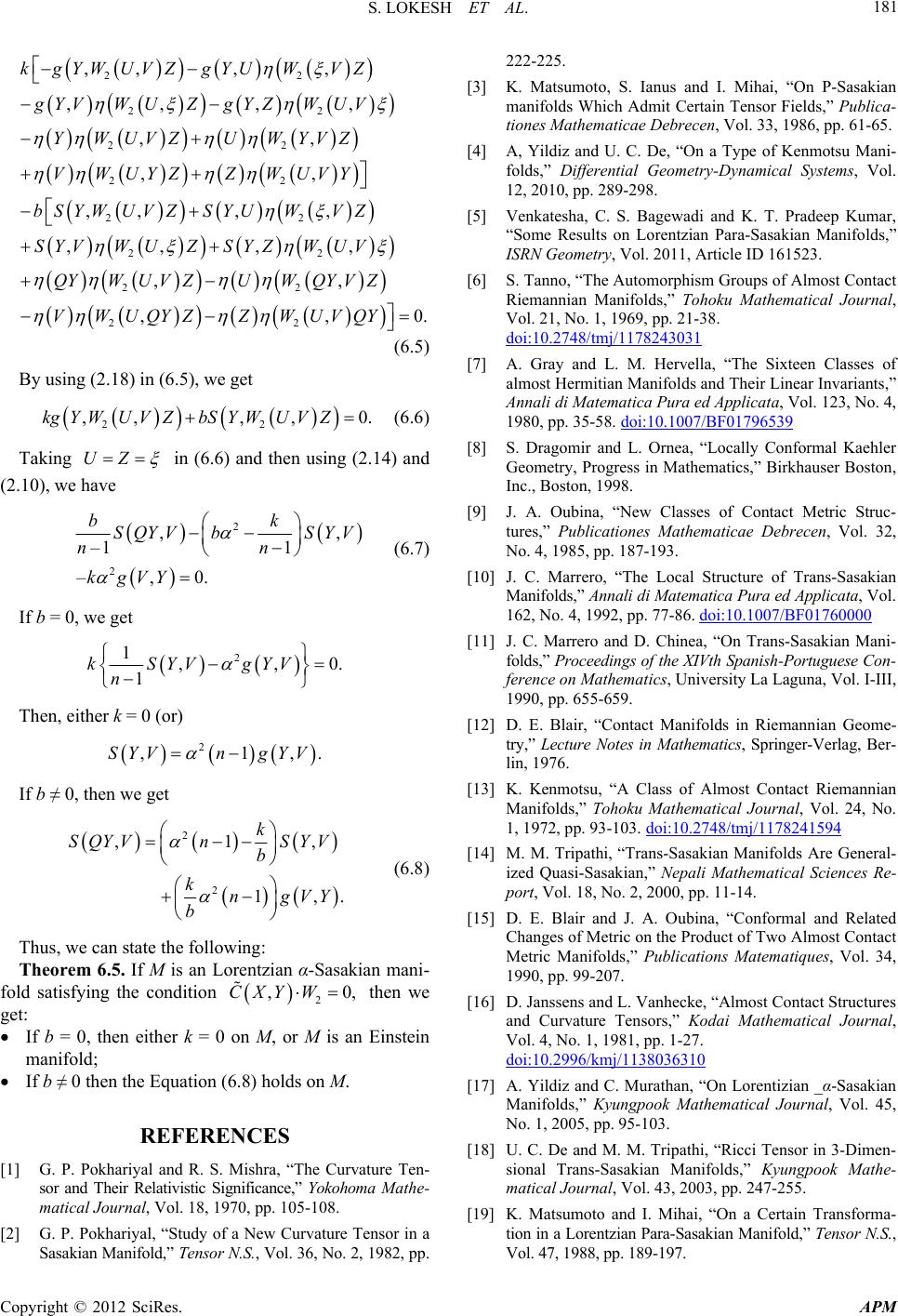

S. LOKESH ET AL. 181



 


    
    



 


     
    
2
22
22
22
2
22
22
22
,, ,
,,,
,,
,,
,, ,
,,,
,
,
kgYWUVZg YUW
gYVW UZgYZW
YWUVZUWY
VWUYZ ZWU
bS YWUVZSYUW
SYVW UZSYZW
QYWUVZUWQ
VWUQYZ ZW

 
 
 

 
 
 















 
 




 
 
2
2
,
,
,
,
,
,0.
V Z
UV
VZ
VY
V Z
UV
YVZ
UVQY







(6.5)
By using (2.18) in (6.5), we get
 


2
,, 0.U VZ
UZ
2
,,kgY WU VZbSY W (6.6)
Taking

 in (6.6) and then using (2.14) and
(2.10), we have
 
,
1
bk
SYV
n




2
2
,
–1
–,0.
SQYV b
n
kgVY






(6.7)
If b = 0, we get

2
1
1
kSYV
n




,, 0.gYV





,1,.n gYV

Then, either k = 0 (or)

2
SYV 
If b ≠ 0, then we get
 

,
1,.
kS YV
b
ngVY








2
,0,Y W
2
2
,1S QYVn
k
b





(6.8)
Thus, we can state the following:
Theorem 6.5. If M is an Lorentzian α-Sasakian mani-
fold satisfying the condition then we
get:
CX

 If b = 0, then either k = 0 on M, or M is an Einstein
manifold;
 If b ≠ 0 then the Equation (6.8) holds on M.
REFERENCES
[1] G. P. Pokhariyal and R. S. Mishra, “The Curvature Ten-
sor and Their Relativistic Significance,” Yokohoma Mathe-
matical Journal, Vol. 18, 1970, pp. 105-108.
[2] G. P. Pokhariyal, “Study of a New Curvature Tensor in a
Sasakian Manifold,” Tensor N.S., Vol. 36, No. 2, 1982, pp.
222-225.
[3] K. Matsumoto, S. Ianus and I. Mihai, “On P-Sasakian
manifolds Which Admit Certain Tensor Fields,” Publica-
tiones Mathematicae Debrecen, Vol. 33, 1986, pp. 61-65.
[4] A, Yildiz and U. C. De, “On a Type of Kenmotsu Mani-
folds,” Differential Geometry-Dynamical Systems, Vol.
12, 2010, pp. 289-298.
[5] Venkatesha, C. S. Bagewadi and K. T. Pradeep Kumar,
“Some Results on Lorentzian Para-Sasakian Manifolds,”
ISRN Geometry, Vol. 2011, Article ID 161523.
[6] S. Tanno, “The Automorphism Groups of Almost Contact
Riemannian Manifolds,” Tohoku Mathematical Journal,
Vol. 21, No. 1, 1969, pp. 21-38.
doi:10.2748/tmj/1178243031
[7] A. Gray and L. M. Hervella, “The Sixteen Classes of
almost Hermitian Manifolds and Their Linear Invariants,”
Annali di Matematica Pura ed Applicata, Vol. 123, No. 4,
1980, pp. 35-58. doi:10.1007/BF01796539
[8] S. Dragomir and L. Ornea, “Locally Conformal Kaehler
Geometry, Progress in Mathematics,” Birkhauser Boston,
Inc., Boston, 1998.
[9] J. A. Oubina, “New Classes of Contact Metric Struc-
tures,” Publicationes Mathematicae Debrecen, Vol. 32,
No. 4, 1985, pp. 187-193.
[10] J. C. Marrero, “The Local Structure of Trans-Sasakian
Manifolds,” Annali di Matematica Pura ed Applicata, Vol.
162, No. 4, 1992, pp. 77-86. doi:10.1007/BF01760000
[11] J. C. Marrero and D. Chinea, “On Trans-Sasakian Mani-
folds,” Proceedings of the XIVth Spanish-Portuguese Con-
ference on Mathematics, University La Laguna, Vol. I-III,
1990, pp. 655-659.
[12] D. E. Blair, “Contact Manifolds in Riemannian Geome-
try,” Lecture Notes in Mathematics, Springer-Verlag, Ber-
lin, 1976.
[13] K. Kenmotsu, “A Class of Almost Contact Riemannian
Manifolds,” Tohoku Mathematical Journal, Vol. 24, No.
1, 1972, pp. 93-103. doi:10.2748/tmj/1178241594
[14] M. M. Tripathi, “Trans-Sasakian Manifolds Are General-
ized Quasi-Sasakian,” Nepali Mathematical Sciences Re-
port, Vol. 18, No. 2, 2000, pp. 11-14.
[15] D. E. Blair and J. A. Oubina, “Conformal and Related
Changes of Metric on the Product of Two Almost Contact
Metric Manifolds,” Publications Matematiques, Vol. 34,
1990, pp. 99-207.
[16] D. Janssens and L. Vanhecke, “Almost Contact Structures
and Curvature Tensors,” Kodai Mathematical Journal,
Vol. 4, No. 1, 1981, pp. 1-27.
doi:10.2996/kmj/1138036310
[17] A. Yildiz and C. Murathan, “On Lorentizian _α-Sasakian
Manifolds,” Kyungpook Mathematical Journal, Vol. 45,
No. 1, 2005, pp. 95-103.
[18] U. C. De and M. M. Tripathi, “Ricci Tensor in 3-Dimen-
sional Trans-Sasakian Manifolds,” Kyungpook Mathe-
matical Journal, Vol. 43, 2003, pp. 247-255.
[19] K. Matsumoto and I. Mihai, “On a Certain Transforma-
tion in a Lorentzian Para-Sasakian Manifold,” Tensor N.S.,
Vol. 47, 1988, pp. 189-197.

S. LOKESH ET AL.
182
[20] K. Yano and M. Kon, “Structures on Manifolds,” Series
in Pure Mathematics, Vol. 3, World Scientific Publishing
Co., Singapore, 1984.
[21] G. P. Pokhariyal and R. S. Mishra, “Curvature Tensor and
Their Relativistic Significance II,” Yokohama Mathemati-
cal Journal, Vol. 19, 1971, pp. 97-103.