Modern Economy, 2010, 1, 17-42
doi:10.4236/me.2010.11002 Published Online May 2010 (http://www.SciRP.org/journal/me)
Is the Great Moderation Ending?
——UK and US Evidence
Giorgio Canarella1,2, Wen-Shwo Fang3, Stephen M. Miller2, Stephen K. Pollard1
1California State University, Los Angeles, USA
2University of Nevada, Las Vegas, USA
3Feng Chia University Taichung, Taiwan, China
[e-mail], alstatela.edu
Received March 3, 2010; revised March 25, 2010; accepted April 5, 2010
Abstract
The Great Moderation, the significant decline in the variability of economic activity, provides a most re-
markable feature of the macroeconomic landscape in the last twenty years. A number of papers document the
beginning of the Great Moderation in the US and the UK. In this paper, we use the Markov regime-switching
models to document the end of the Great Moderation. The Great Moderation in the US and the UK begin at
different point in time. The explanations for the Great Moderation fall into generally three different catego-
ries—good monetary policy, improved inventory management, or good luck. The end of the Great Modera-
tion, however, occurs at approximately the same time in both the US and the UK. It seems unlikely that good
monetary policy would turn into bad policy or that better inventory management would turn into worse
management. Rather, the likely explanation comes from bad luck. Two likely culprits exist—energy-price
and housing-price shocks.
Keywords: Great Moderation, Regime Switching, SWARCH
1. Introduction
Time-series patterns of real output growth, like many
other economic and financial time series, exhibit periods
of high volatility followed by periods of low volatility.
Generalized autoregressive conditional heteroskedastic-
ity (GARCH) models, based on the seminal works of [1]
and [2], accommodate this phenomenon by explicitly
modeling the tendency for more large (small) changes in
the underlying time series to follow large (small)
changes, thus permitting estimation of the observed vola-
tility clustering. Problems in estimating GARCH models,
however, arise if the underlying volatility process ex-
periences structural breaks, especially shifts in the over-
all level of volatility. The empirical literature shows that
the sum of the estimated GARCH coefficients nearly
equals, or even exceeds, one, implying a non-stationary
variance process (i.e., integrated GARCH or IGARCH
process). According to [3], this high volatility persistence
of shocks in single regime GARCH models may
reflect structural changes in the variance process. For
example, if high, but constant (homoskedastic), variance
for some time switches to a low, but constant, variance,
then combining such high and low homoskedastic vola-
tility periods produces spurious overall volatility persis-
tence. That is, a GARCH model does not differentiate
between homoskedastic volatility sub-periods, but iden-
tifies high persistence and heteroskedasticity across the
full sample. As such, disregarding regime changes leads
to a misspecified GARCH model. The misspecified
GARCH model systematically overstated the persistence
of volatility shocks (see [4,5]).
Commonly, researchers deal with such structural
breaks by introducing dummy variables for given sub-
periods reflecting the change in the level of volatility.
For example, Reference [6] develops a test based on the
modified iterated cumulated sums of squares (ICSS) al-
gorithm (see [7]) and analyzes real GDP growth rates for
six OECD countries (Canada, Germany, Italy, Japan, the
United Kingdom, and the United States) from 1960 to
2006 and find a number of structural breaks in the data.1
The modified ICSS algorithm, however, suffers from an
1In early work, Reference [8] introduces a similar methodology fo
r
considering the Great Moderation in the US.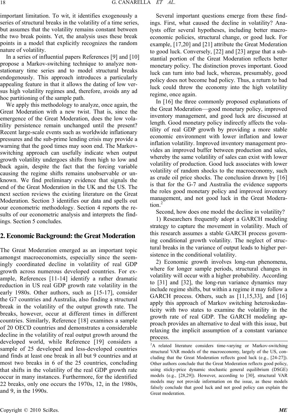

G. CANARELLA ET AL. 18
important limitation. To wit, it identifies exogenously a
series of structural breaks in the volatility of a time series,
but assumes that the volatility remains constant between
the two break points. Yet, the analysis uses these break
points in a model that explicitly recognizes the random
nature of volatility.
In a series of influential papers References [9] and [10]
propose a Markov-switching technique to analyze non-
stationary time series and to model structural breaks
endogenously. This approach introduces a particularly
appealing feature in that it allows the dating of low ver-
sus high volatility regimes and, therefore, avoids any ad
hoc partitioning of the sample path.
We apply this methodology to analyze, once again, the
Great Moderation with a new twist. That is, since the
emergence of the Great Moderation, does the low vola-
tility persistence remain unchanged until the present?
Recent large-scale events such as worldwide inflationary
pressures and the sub-prime lending crisis may provide a
warning that the good times may soon end. The Markov-
switching approach can usefully indicate when output
growth volatility undergoes shifts from high to low and
back again, despite the fact that the forcing variable
causing the regime shifts remains unobservable or un-
known. We find preliminary evidence that signals the
end of the Great Moderation in the UK and the US. The
next section reviews the existing literature on the Great
Moderation. Section 3 identifies our data and spells out
our econometric methodology. Section 4 reports the re-
sults of our econometric analysis and interprets the find-
ings. Section 5 concludes.
2. Economic Background: the Great Moderation
The Great Moderation emerged as an important topic
amongst macroeconomists, especially since the seem-
ingly coordinated decline in volatility of real GDP
growth across numerous developed countries. For ex-
ample, References [11-14] identify a rather dramatic
reduction in US real GDP growth rate volatility in the
early 1980s. Other authors, such as [15-17], consider
the G7 countries and Australia, also finding a structural
break in the volatility of the output growth rate. The
breaks, however, occur at different times in different
countries. Similarly, Reference [18] examines a sample
of 20 OECD countries and demonstrates a considerable
decline in the volatility of real output growth around the
developed world, while Reference [19] considers a
sample of 25 developed and less-developed countries
and finds at least one break in all but 9 countries and at
most two breaks in 6 of the 25 countries, concluding
that shifts in the volatility of the real GDP growth rate
occur in many instances. Furthermore, for the identified
22 breaks, only one occurs the 1970s, 12, in the 1980s,
and 9, in the 1990s.
Several important questions emerge from these find-
ings. First, what caused the decline in volatility? Ana-
lysts offer several hypotheses, including better macro-
economic policies, structural change, or good luck. For
example, [17,20] and [21] attribute the Great Moderation
to good luck. Conversely, [22] and [23] argue that a sub-
stantial portion of the Great Moderation reflects better
monetary policy. The distinction proves important. Good
luck can turn into bad luck, whereas, presumably, good
policy does not become bad policy. Thus, a return to bad
luck could throw the economy into the high volatility
regime, once again.
In [16] the three commonly proposed explanations of
the Great Moderation—good monetary policy, improved
inventory management, and good luck are discussed at
length. Good monetary policy indirectly affects the vola-
tility of real GDP growth by providing a more stable
economic environment with lower inflation and lower
inflation volatility. Improved inventory management pro-
vides an improved buffer between production and sales,
whereby the same volatility of sales can exist with lower
volatility of production. Good luck associates with lower
volatility of random shocks to the macroeconomy, such
as crude oil price shocks. The conclusion drawn by [16]
is that for the G-7 and Australia the evidence supports
the roles good monetary policy and improved inventory
management, and not good luck in the Great Modera-
tion.2
Second, how does one model the decline in volatility?
1) Researchers frequently adopt a GARCH modeling
strategy to capture the movement in volatility. Much of
this research assumes a stable GARCH process govern-
ing conditional growth volatility. The neglect of struc-
tural breaks in the variance of output leads to higher per-
sistence in the conditional volatility.
2) Economic growth involves long-run phenomena,
where for longer sample periods, structural changes in
volatility will occur with a higher probability. According
to [31] and [32], the long-run variance dynamics may
include regime shifts, but within a regime it may follow a
GARCH process. Others, such as [11,15,33], and [16]
apply this approach of Markov switching heteroskedas-
ticity with two states to examine the volatility in the
growth rate of real GDP. The GARCH modeling ap-
proach provides an alternative to deal with this issue, but
relaxing the implicit assumption of a constant variance
process.
2A related literature considers time-varying or Markov-switching
structural VAR models of the macroeconomy, largely of the US, con-
cluding that the Great Moderation reflects good luck (e.g., [24-27]).
Other authors conclude that the Great Moderation reflects good policy,
using sticky-price dynamic stochastic general equilibrium (DSGE)
models (e.g., [28,29]). However, according to [30], structural VAR
models may not provide information on the issue, as these models
falsely conclude that good luck and not good policy can explain the
Great moderation.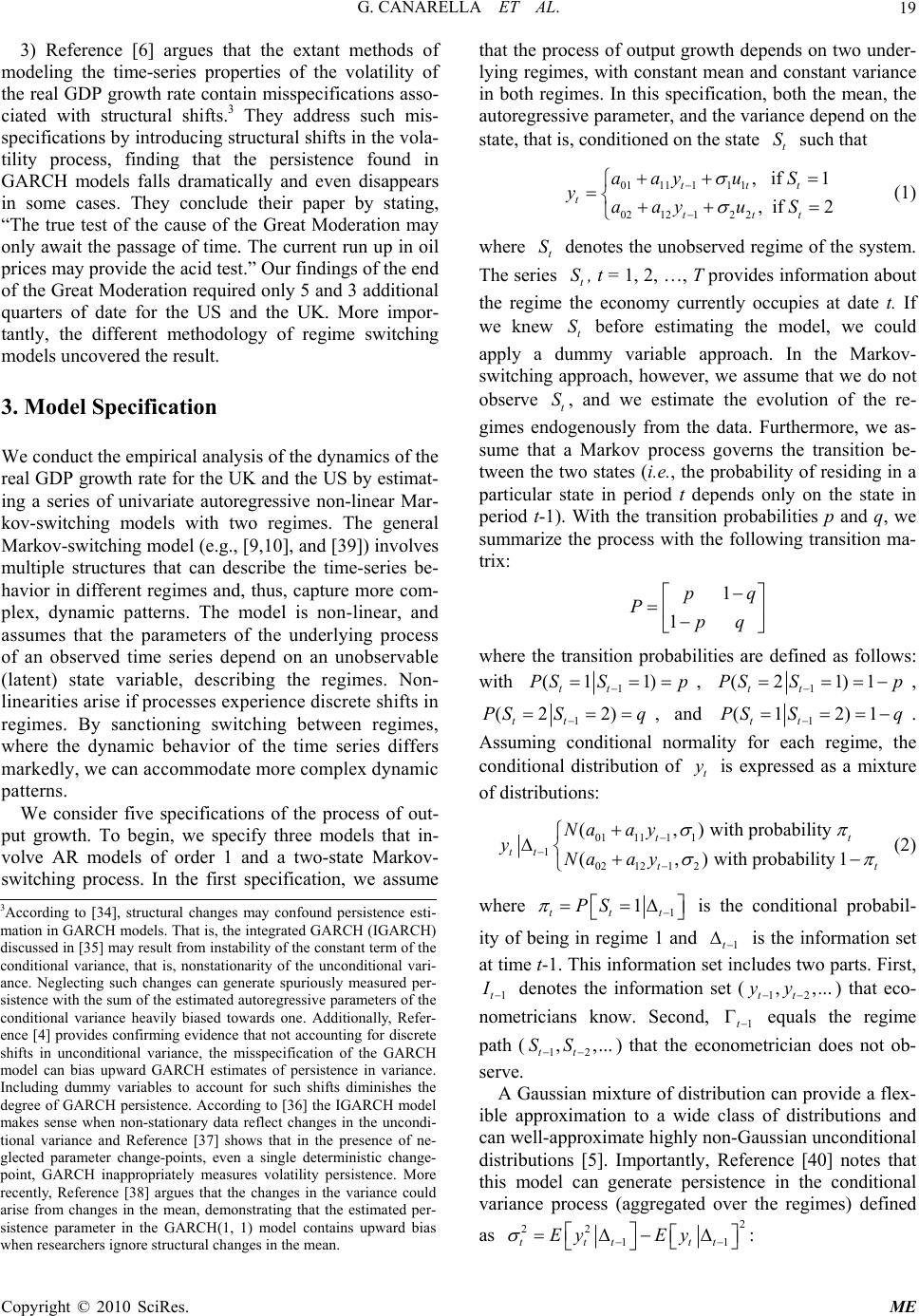

G. CANARELLA ET AL.19
3) Reference [6] argues that the extant methods of
modeling the time-series properties of the volatility of
the real GDP growth rate contain misspecifications asso-
ciated with structural shifts.3 They address such mis-
specifications by introducing structural shifts in the vola-
tility process, finding that the persistence found in
GARCH models falls dramatically and even disappears
in some cases. They conclude their paper by stating,
“The true test of the cause of the Great Moderation may
only await the passage of time. The current run up in oil
prices may provide the acid test.” Our findings of the end
of the Great Moderation required only 5 and 3 additional
quarters of date for the US and the UK. More impor-
tantly, the different methodology of regime switching
models uncovered the result.
3. Model Specification
We conduct the empirical analysis of the dynamics of the
real GDP growth rate for the UK and the US by estimat-
ing a series of univariate autoregressive non-linear Mar-
kov-switching models with two regimes. The general
Markov-switching model (e.g., [9,10], and [39]) involves
multiple structures that can describe the time-series be-
havior in different regimes and, thus, capture more com-
plex, dynamic patterns. The model is non-linear, and
assumes that the parameters of the underlying process
of an observed time series depend on an unobservable
(latent) state variable, describing the regimes. Non-
linearities arise if processes experience discrete shifts in
regimes. By sanctioning switching between regimes,
where the dynamic behavior of the time series differs
markedly, we can accommodate more complex dynamic
patterns.
We consider five specifications of the process of out-
put growth. To begin, we specify three models that in-
volve AR models of order 1 and a two-state Markov-
switching process. In the first specification, we assume
that the process of output growth depends on two under-
lying regimes, with constant mean and constant variance
in both regimes. In this specification, both the mean, the
autoregressive parameter, and the variance depend on the
state, that is, conditioned on the state such that
t
S
011111 1
021212 2
, if 1
, if 2
ttt
t
ttt
aayu S
yaayu S










 (1)
where denotes the unobserved regime of the system.
The series , t = 1, 2, …, T provides information about
the regime the economy currently occupies at date t. If
we knew before estimating the model, we could
apply a dummy variable approach. In the Markov-
switching approach, however, we assume that we do not
observe , and we estimate the evolution of the re-
gimes endogenously from the data. Furthermore, we as-
sume that a Markov process governs the transition be-
tween the two states (i.e., the probability of residing in a
particular state in period t depends only on the state in
period t-1). With the transition probabilities p and q, we
summarize the process with the following transition ma-
trix:
t
S
S
t
S
t
S
t
1
1
pq
Ppq









where the transition probabilities are defined as follows:
with 1
(1 1)
tt
PS Sp


 , 1 (2 1)1
tt
PS Sp

,
1
(2 2)
tt
PS Sq


, and 1 (1 2)1
tt
PS Sq

.
Assuming conditional normality for each regime, the
conditional distribution of is expressed as a mixture
of distributions:
t
y
01111 1
1
02121 2
(,) with probability
(,) with probability 1
tt
tt
tt
Naa y
yNaa y











 (2)
where 1 1
ttt
PS 





 is the conditional probabil-
ity of being in regime 1 and is the information set
at time t-1. This information set includes two parts. First,
1t

1t
I

denotes the information set () that eco-
nometricians know. Second, equals the regime
path () that the econometrician does not ob-
serve.
12
, ,...
tt
yy

1t

12
, ,...
tt
SS

3According to [34], structural changes may confound persistence esti-
mation in GARCH models. That is, the integrated GARCH (IGARCH)
discussed in [35] may result from instability of the constant term of the
conditional variance, that is, nonstationarity of the unconditional vari-
ance. Neglecting such changes can generate spuriously measured per-
sistence with the sum of the estimated autoregressive parameters of the
conditional variance heavily biased towards one. Additionally, Refer-
ence [4] provides confirming evidence that not accounting for discrete
shifts in unconditional variance, the misspecification of the GARCH
model can bias upward GARCH estimates of persistence in variance.
Including dummy variables to account for such shifts diminishes the
degree of GARCH persistence. According to [36] the IGARCH model
makes sense when non-stationary data reflect changes in the uncondi-
tional variance and Reference [37] shows that in the presence of ne-
glected parameter change-points, even a single deterministic change-
p
oint, GARCH inappropriately measures volatility persistence. More
recently, Reference [38] argues that the changes in the variance could
arise from changes in the mean, demonstrating that the estimated per-
sistence parameter in the GARCH(1, 1) model contains upward bias
when researchers ignore structural changes in the mean.
A Gaussian mixture of distribution can provide a flex-
ible approximation to a wide class of distributions and
can well-approximate highly non-Gaussian unconditional
distributions [5]. Importantly, Reference [40] notes that
this model can generate persistence in the conditional
variance process (aggregated over the regimes) defined
as 2
22
11ttt tt
Ey Ey 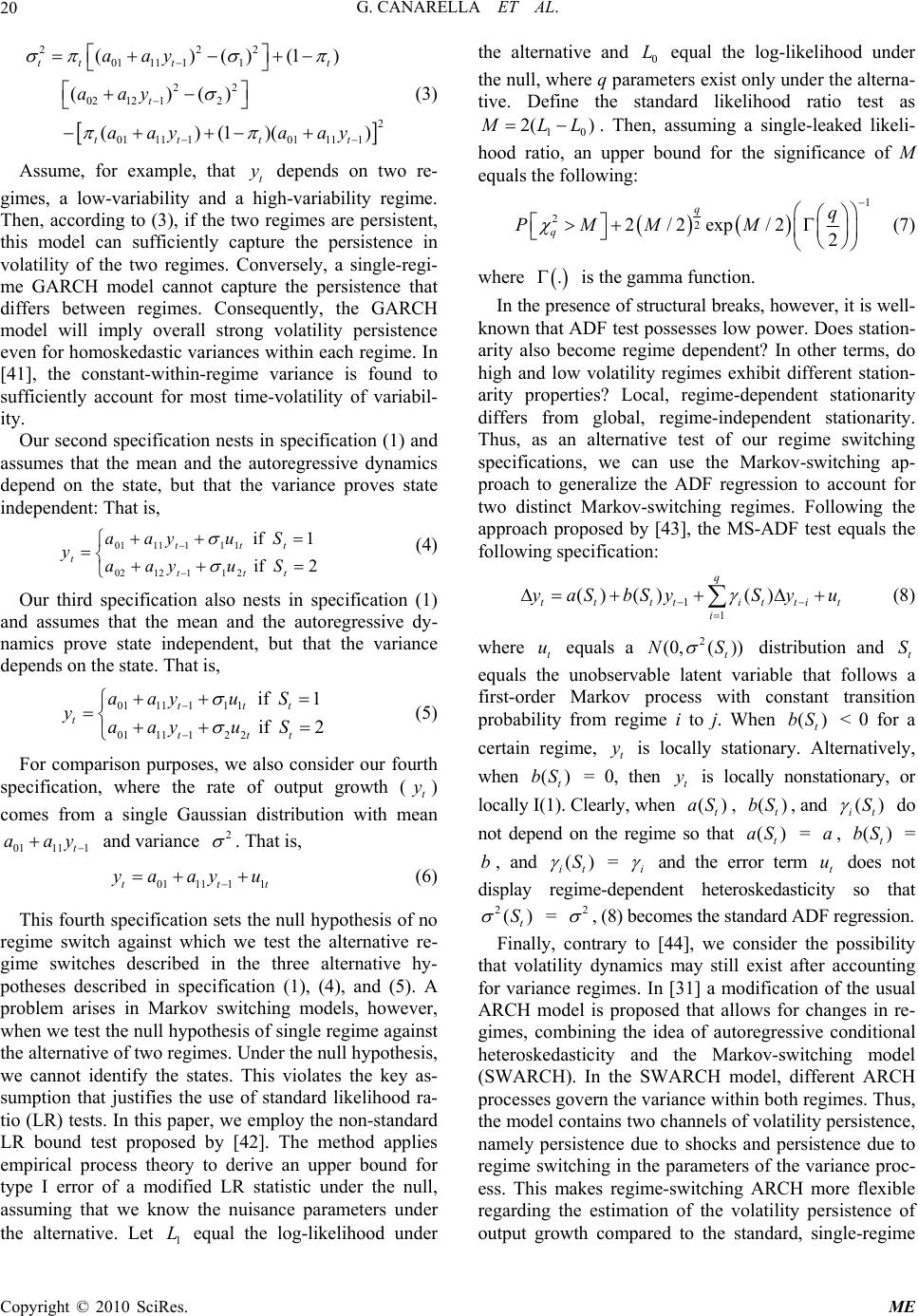






 :

G. CANARELLA ET AL. 20


222
0111 11
22
0212 12
2
0111 10111 1
()()(1)
()()
()(1)()
tt tt
t
tttt
aay
aay
aay aay
 






 






(3)
Assume, for example, that depends on two re-
gimes, a low-variability and a high-variability regime.
Then, according to (3), if the two regimes are persistent,
this model can sufficiently capture the persistence in
volatility of the two regimes. Conversely, a single-regi-
me GARCH model cannot capture the persistence that
differs between regimes. Consequently, the GARCH
model will imply overall strong volatility persistence
even for homoskedastic variances within each regime. In
[41], the constant-within-regime variance is found to
sufficiently account for most time-volatility of variabil-
ity.
t
y
Our second specification nests in specification (1) and
assumes that the mean and the autoregressive dynamics
depend on the state, but that the variance proves state
independent: That is,








2if
1if
2111202
1111101
ttt
ttt
tSuyaa
Suyaa
y


(4)
Our third specification also nests in specification (1)
and assumes that the mean and the autoregressive dy-
namics prove state independent, but that the variance
depends on the state. That is,
011111 1
011112 2
if 1
if 2
ttt
t
ttt
aayu S
yaayu S




 

 
 (5)
For comparison purposes, we also consider our fourth
specification, where the rate of output growth ()
comes from a single Gaussian distribution with mean
and variance
t
y
0111 1t
aay

2

. That is,
0111 11tt
ya ayu

 
t
(6)
This fourth specification sets the null hypothesis of no
regime switch against which we test the alternative re-
gime switches described in the three alternative hy-
potheses described in specification (1), (4), and (5). A
problem arises in Markov switching models, however,
when we test the null hypothesis of single regime against
the alternative of two regimes. Under the null hypothesis,
we cannot identify the states. This violates the key as-
sumption that justifies the use of standard likelihood ra-
tio (LR) tests. In this paper, we employ the non-standard
LR bound test proposed by [42]. The method applies
empirical process theory to derive an upper bound for
type I error of a modified LR statistic under the null,
assuming that we know the nuisance parameters under
the alternative. Let equal the log-likelihood under
the alternative and equal the log-likelihood under
the null, where q parameters exist only under the alterna-
tive. Define the standard likelihood ratio test as
1
L
0
L
10
2( )
M
LL

. Then, assuming a single-leaked likeli-
hood ratio, an upper bound for the significance of M
equals the following:

1

2
q
PM

2
2exp/2 2
qq
M M2/ 

 
 



 (7)
where


.

is the gamma function.
In the presence of structural breaks, however, it is well-
known that ADF test possesses low power. Does station-
arity also become regime dependent? In other terms, do
high and low volatility regimes exhibit different station-
arity properties? Local, regime-dependent stationarity
differs from global, regime-independent stationarity.
Thus, as an alternative test of our regime switching
specifications, we can use the Markov-switching ap-
proach to generalize the ADF regression to account for
two distinct Markov-switching regimes. Following the
approach proposed by [43], the MS-ADF test equals the
following specification:
1
1
) ()
q
tt itti
i
ySy u 


(
tt
yaS()bSt


 (8)
where equals a distribution and
equals the unobservable latent variable that follows a
first-order Markov process with constant transition
probability from regime i to j. When < 0 for a
certain regime, is locally stationary. Alternatively,
when = 0, then is locally nonstationary, or
locally I(1). Clearly, when , , and
t
u
()
t
bS
2
(0,( ))
t
NS 
t
y
()
t
aS
t
S
)
()
t
bS
)
t
y
(
t
bS (
it
S

do
not depend on the regime so that = , =
, and
(
t
aS)a(
t
bS)
b()
it
S

= i

and the error term does not
display regime-dependent heteroskedasticity so that
=
t
u
2()
t
S 
2

, (8) becomes the standard ADF regression.
Finally, contrary to [44], we consider the possibility
that volatility dynamics may still exist after accounting
for variance regimes. In [31] a modification of the usual
ARCH model is proposed that allows for changes in re-
gimes, combining the idea of autoregressive conditional
heteroskedasticity and the Markov-switching model
(SWARCH). In the SWARCH model, different ARCH
processes govern the variance within both regimes. Thus,
the model contains two channels of volatility persistence,
namely persistence due to shocks and persistence due to
regime switching in the parameters of the variance proc-
ess. This makes regime-switching ARCH more flexible
regarding the estimation of the volatility persistence of
output growth compared to the standard, single-regime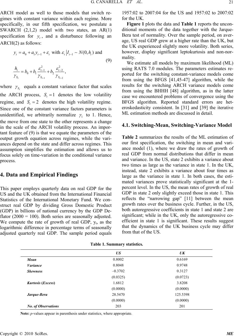

G. CANARELLA ET AL. 21
ARCH model as well to those models that switch re-
gimes with constant variance within each regime. More
specifically, in our fifth specification, we postulate a
SWARCH (2,1,2) model with two states, an AR(1)
specification for , and a disturbance following an
ARCH(2) as follows:
t
y
1957:02 to 2007:04 for the US and 1957:02 to 2007:02
for the UK.
Figure 1 plots the data and Table 1 reports the uncon-
ditional moments of the data together with the Jarque-
Bera test of normality. Over the sample period, on aver-
age, US real GDP grew at a higher rate than the UK, but
the UK experienced slightly more volatility. Both series,
however, display significant leptokurtosis and non-nor-
mality.
12
011 1
22
12
01 2
with (0,) and
,
ttt
tttttt
ttt
SSS
yaayI Nh
hbb b






 
 

(9) We estimate all models by maximum likelihood (ML)
using RATS 7.0 modules. The parameters estimates re-
ported for the switching constant-variance models come
from using the BFGS [41,45-47] algorithm, while the
results for the switching ARCH variance models come
from using the BHHH [48] algorithm, as in the latter
case we encountered problems of convergence using the
BFGS algorithm. Reported standard errors are het-
eroskedasticity consistent. In [31] and [39] the iterative
ML estimation methods are discussed in detail.
where t
S

equals a constant variance factor that scales
the ARCH process, denotes the low volatility
regime, and denotes the high volatility regime.
Since one of the constant variance factors parameters is
unidentified, we arbitrarily normalize
1
t
S
2
t
S
1

to 1. Hence,
the move from one state to the other represents a change
in the scale of the ARCH volatility process. An impor-
tant feature of (9) is that we equate the parameters of the
4.1. Switching-Mean, Switching-Variance Model
Table 2 summarizes the results of the ML estimation of
our first specification, the switching in mean and vari-
ance model (1), where we draw the rates of growth of
real GDP from normal distributions that differ in mean
and variance. In the US, state 2 exhibits a variance about
two times as large as the variance in state 1. In the UK,
instead, state 2 exhibits a variance about four times as
large as the variance in state 1. In both cases, the esti-
mated variances prove statistically significant at the 1-
percent level. In the US, the mean rates of growth of real
GDP in state 2 only slightly exceed those in state 1. This
reflects the “narrowing gap” [11] between the mean
growth rates over the business cycle. Further, in the US,
both autoregressive coefficients in state 1 and state 2 are
significant; while in the UK, only the autoregressive co-
efficient in state 1 is significant. These results suggest
that the dynamics of the UK business cycle may differ
from that of the US.
output growth equation across regimes, while the vari-
ances depend on the state and differ across regimes. This
assumption simplifies the estimation and allows us to
focus solely on time-variation in the conditional variance
process.
4. Data and Empirical Findings
This paper employs quarterly data on real GDP for the
US and the UK obtained from the International Financial
Statistics of the International Monetary Fund. We con-
struct real GDP by dividing Gross Domestic Product
(GDP) in billions of national currency by the GDP De-
flator (2000 = 100). Both series are seasonally adjusted.
We compute the rate of growth of real GDP, yt, as the
logarithmic difference in percentage terms of seasonally
adjusted quarterly real GDP. The sample period equals
Table 1. Summary statistics.
US UK
Mean 0.8002 0.6169
Variance 0.8048 0.9748
Skewness –0.3702 0.3127
(0.0325) (0.0723)
Kurtosis (Excess) 1.6812 3.8208
(0.0000) (0.0000)
Jarque-Bera 28.5470 125.5398
(0.0000) (0.0000)
No. of Observations 203 201
Note: p-values appear in parenthesis under statistics, where appropriate.

G. CANARELLA ET AL. 22
-3
-2
-1
0
1
2
3
4
1957 195919621964 1967 196919721974 19771979 19821984 19871989 19921994 19971999 20022004 2007
(a) US (1957:02 to 2007:04)
-3
-2
-1
0
1
2
3
4
5
195719591962196419671969 1972197419771979198219841987198919921994 19971999200220042007
(b) UK (1957:02 to 2007:02)
Figure 1. Real GDP growth rates.

G. CANARELLA ET AL. 23
Table 2. Parameter estimates and related statistics for switching-variance, switching-mean model.
US UK
Parameter Estimate t-statistic Estimate t-statistic
01
a 0.5719* 5.9323 0.2722* 4.5452
02
a 0.6046* 4.4723 0.6809* 6.2420
11
a 0.2362** 2.0627 0.5964* 7.5544
12
a 0.2956* 3.1029 –0.1077 –1.2289
1

0.4780* 12.7832 0.2758* 11.5809
2

1.0825* 14.3776 1.1716* 15.1208
P 0.9941* 131.4765 0.9932* 110.9160
Q 0.9945* 144.9275 0.9953* 175.3622
Log-likelihood –230.4212 –225.2013
AIC 472.8424 262.4026
SIC 524.5416 513.9824
HQ 480.8735 470.4112
Diagnostic Tests Statistic p-value Statistic p-value
Q1(4) 6.542256 0.1621 3.1652 0.5306
Q1(8) 10.542728 0.2290 10.3391 0.2420
Q2(4) 2.613116 0.6245 2.9133 0.5724
Q2(8) 6.443422 0.5977 5.0920 0.7477
Skewness –0.361758 0.0372 –0.0530 0.7610
Kurtosis (excess) 0.598052 0.0881 1.3582 0.0001
Jarque-Bera 7.416269 0.0245㎡ 15.4679 0.0004
Note: The AIC, SIC, and HQ equal Akaike, Schwartz-Bayesian, and Hannan-Quinn information criterion. The Q1(k) and Q2(k) equal Ljung-Box
Q-statistics, testing for standardized residuals and squared standardized residuals for autocorrelations up to k lags.
* denotes 1% significance level.
** denotes 5% significance level.
Table 2 also reports the results of a series of diagnos-
tic tests. Q1(4) and Q1(8) equal the Ljung-Box statistics
for the joint significance of autocorrelations of standard-
ized residuals for the first 4 and 8 lags, respectively, and
Q2(4) and Q2(8) equal the Ljung-Box statistics for the
joint significance of autocorrelations of squared stan-
dardized residuals for the same number of lags. Under
the null hypothesis of zero autocorrelation, each statistic
is distributed as a chi-square variable with 4 and 8 de-
grees of freedom, respectively. The Ljung-Box statistics
indicate that the regime switching model can success-
fully capture the serial correlation in the conditional
mean and variance of the US and UK rates of real GDP
growth and show no evidence of non-linear dependencies
or omitted ARCH effects. This finding is particularly
interesting because growth rates of real GDP show
strong ARCH effects, as widely documented [49-51].
Further, the regime-switching model reduces the excess
kurtosis of standardized residuals relative to the excess
kurtosis present in the actual data, although some degree
of leptokurtosis remains in the UK results.4
The high persistence of the regimes, where the transi-
tion probabilities p and q lie close to 1, proves an impor-
tant feature of the estimation. That is, these high prob-
abilities indicate that if the economy begins in either
state 1 or state 2, it will likely remain in that state.
Figures 2 and 3 provide a visual interpretation of the
results, showing how the probability of being in either
state 1 or state 2 evolves over the sample.
We base our inference on the full sample and the
estimated ML parameters. We calculate these “smo-
othed” probabilities, Pr[1 ]
t
S
T
and in contrast
Pr[2 ]
t
ST

 for each quarter based on the knowledge
of the complete sample of data, in contrast to the “ex
ante” probabilities, Pr[1 ]
t
St

 and Pr[2 ]
tt
S

,
which we calculate for each quarter based on information
available up to date . The “smoothed” probabilities
provide a relatively objective method of dating major
shifts in conditional volatility. In Hamilton [10] a direct
method is proposed for dating regime switches, whereby
an observation belongs to a given state if the corre-
sponding smoothed probability exceeds 0.5. The
“smoothed” probability in Figures 2 and 3 strongly in-
dicate the presence of two regimes. Both for the US and
the UK, the probabilities remain extremely close to one
or zero, indicating that the non-linear filter that generates
the “smoothed” probabilities does reflect an underlying
switching process rather than simply fitting parameters in
an ad hoc manner.
t
4Using a different methodology, Reference [6] finds similar results.

G. CANARELLA ET AL. 24
0
0.1
0.2
0.3
0.4
0.5
0.6
0.7
0.8
0.9
1
1957 19591962196419671969197219741977197919821984 198719891992199419971999 200220042007
(a) US
0
0.1
0.2
0.3
0.4
0.5
0.6
0.7
0.8
0.9
1
1957 19591962 1964 19671969 19721974 1977 1979 19821984 19871989 1992 19941997 1999 20022004 2007
(b) UK
Figure 2. Smoothed probability of low volatility in state 1 (switching-mean and -variance model).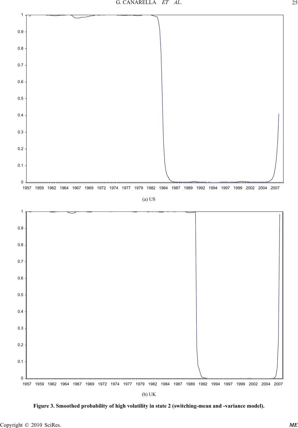

G. CANARELLA ET AL.25
0
0.1
0.2
0.3
0.4
0.5
0.6
0.7
0.8
0.9
1
1957 19591962 196419671969 19721974 1977197919821984 19871989199219941997 19992002 20042007
(a) US
0
0.1
0.2
0.3
0.4
0.5
0.6
0.7
0.8
0.9
1
1957 1959 19621964 1967 1969 19721974 1977 1979 19821984 1987 19891992 1994 1997 1999 20022004 2007
(b) UK
Figure 3. Smoothed probability of high volatility in state 2 (switching-mean and -variance model).

G. CANARELLA ET AL. 26
The evidence favoring the ending of the Great Mod-
eration appears stronger in the UK case. In 1990:04, the
probability of state 1 increases to 0.81 from 0.000001 in
the previous period and remains close to 0.99 until
2006:04, at which time the first slight decline occurs,
from 0.98 in 2006:03 to 0.93 in 2006:04. This probability
declines dramatically in the next two quarters, to 0.76 in
2007:01 and 0.01 in 2007:02, the end of the sample pe-
riod for the UK.
More specifically, these figures document the presence
of two significant structural breaks both in the US and
the UK economic growth process. In the US case, the
first structural break occurs in 1984:03 and the second
takes place in 2007:04. On the other hand, in the UK, the
first structural break occurs in 1990:04 and the second in
2007:02. These two dates prove important in determining
the length and duration of the Great Moderation in the
two countries.
Prior to 1984:03 in the US, the probability of state 1
lies numerically extremely close to zero. This means that
from the beginning of the sample through 1983:03, the
US rate of growth of real GDP experiences high volatil-
ity. Beginning in 1984:03, however, the probability of
the low-volatility state 1 switches from 0.08 in 1983:04
to 0.21 in 1984:01, to 0.47 in 1984:02, and to 0.75 in
1984:03. From 1984:04 to 2006:04 this probability re-
mains above 0.95, the period that coincides with the
Great Moderation. Beginning with 2007:01, however,
signs begin to suggest that the Great Moderation may
come to an end (see Figures 2 and 3). The probability of
the low-volatility state 1 starts to decline, in a fast and
swift manner. In 2007:01, the probability of state 1 falls
from nearly one to 0.91. This probability declines further
to 0.86 in 2007:02, then to 0.75 in 2007:03 and finally to
0.59 in 2007:04. While technically still greater than 0.5,
this evidence points to the beginning of the end of the
Great Moderation era in the US.
4.2. Constant-Mean, Constant-Variance Model
Table 3 reports the estimates of the linear AR(1) single-
regime constant-variance model, our fourth specification
(6), and related diagnostic statistics. Clearly, the model
does a poor job of modeling the volatility of both the US
and the UK growth rates of real GDP. The distribution of
the standardized residuals exhibits heavy leptokurticity
and displays a significant departure from normality. Fur-
thermore, significant evidence emerges of second-moment
nonlinear dependencies in the standardized residuals. As
noted by [39], the single-regime model effectively aver-
ages the variance over the sample period so that the
model does a poor job of describing the data in either
regime. This, in turn, induces positive serial correlation
in the standardized squared residuals, as it overstates the
variance in the low-variance regime and understates the
variance in the high-variance regime.
Table 3. Parameter estimates and related statistics for single-regime, constant-variance model.
US UK
Parameter Estimate t-statistic Estimate t-statistic
01
a 0.5736* 7.9804 0.6591* 8.4099
11
a 0.2885* 4.9006 –0.0631 –1.1316

0.7324* 13.2973 0.9687* 16.6574
Log-likelihood –255.1804 –280.6104
AIC 516.3608 567.2208
SIC 542.2104 593.0107
HQ 530.3919 581.2294
Diagnostic Tests Statistic p-value Statistic p-value
Q(4) 2.24512 0.6908 6.3642 0.1735
Q(8) 8.1799 0.4161 15.3956 0.0519
Q2(4) 13.7143 0.0083 17.3848 0.0016
Q2(8) 28.3926 0.0004 20.7653 0.0078
Skewness –0.2495 0.1508 0.3084 0.0772
Kurtosis (excess) 1.6488 0.0000 3.7844 0.0000
Jarque-Bera 24.9777 0.0000 122.5144 0.0000
Note: The AIC, SIC, and HQ equal Akaike, Schwartz-Bayesian, and Hannan-Quinn information criterion. The Q1(k) and Q2(k) equal Ljung-Box
Q-statistics, testing for standardized residuals and squared standardized residuals for autocorrelations up to k lags.
* denotes 1% significance level.
*
* denotes 5% significance level.

G. CANARELLA ET AL. 27
As previously noted, the test of the null hypothesis of
a single-regime constant-variance model against the al-
ternative of a regime-switching model is not straight-
forward. Under the null, only one regime exists in fact
that governs the rate of growth of real GDP. Thus, we
cannot identify the regime staying probabilities p and q.
This makes the asymptotic distribution of the usual tests
(likelihood ratio, Wald and Lagrange multiplier) no
longer chi-square [42,52,53]. To interpret the likelihood
ratio statistics, we appeal to the methods in [15]. Testing
the null of single regime against the alternative of a
switching regime implies that r = 3, where r equals the
number of restrictions (i.e., =, =, and
01
a02 a11 a12 a
1

=2

). From (7), we can calculate that the 0.05 (0.01)
upper bound requires a value of 12.94 (16.91), rather
than the conventional chi-square value of 7.81 (11.30).
Values exceeding this upper bound suggest rejecting the
null hypothesis. The LR test statistics for the US equals
49.51 and for the UK, 110.81. These numbers imply that
we reject the null in both cases, even after invoking the
upper bound in [42]. Thus, these results provide strong
evidence in favor of the two-state regime-switching
specification for the growth rates of real GDP of the US
and the UK.
4.3. Switching-Mean, Constant-Variance Model
Table 4 reports the ML estimates of the switching-mean,
constant-variance model, our second specification (4),
(i.e., 01 a

02
a, 11 a

12
a, but 1

=2

). The large dif-
ference in mean growth rates between the two regimes
provides the most conspicuous feature of the estimates.
The estimates of the transition probabilities imply that
the probability of remaining in the low volatility state 1
remains extremely high for both the US and the UK. The
situation differs for state 2. The probability in the US that
state 2 will persist for more than one quarter equals only
0.1757, while the probability in the UK that state 2 will
persist for more than one quarter equals a value about
four times as high.
Figures 4 and 5 show how the “smoothed” probability
of residing in either state 1 or state 2 evolves over the
sample. The evidence in Figure 4 indicates that when the
probability of residing in the low volatility state 1 devi-
ates from 1, it does so for a short period of time. The
figure reflects this in the sharp spikes at irregular inter-
vals, especially during the mid and late seventies, the
early eighties, and the early nineties. The switch-
ing-mean model improves over the single-regime, con-
Table 4. Parameter estimates and related statistics for switching-mean, constant-variance model.
US UK
Parameter Estimate t-statistic Estimate t-statistic
01
a 0.7249* 9.4073 0.8914* 11.2831
02
a –1.3946* –3.9970 –0.7775* –3.1722
11
a 0.2330* 3.6135 –0.1406** –2.2785
12
a 0.5542** 2.2063 –0.4749* –3.2266

0.7303* 12.1771 0.8294* 18.3436
p 0.9519* 30.8059 0.9658* 58.9268
q 0.1757* 5.7510 0.7436** 2.3222
Log-likelihood –249.2448 –271.9547
AIC 508.4896 553.9094
SIC 551.5722 596.8925
HQ 518.5207 563.9180
Diagnostic Tests Statistic p-value Statistic p-value
Q(4) 2.7166 0.6063 2.6249 0.6224
Q(8) 8.6743 0.3705 14.3417 0.0733
Q2(4) 14.6559 0.0055 13.7299 0.0082
Q2(8) 30.6716 0.0002 19.5367 0.0122
Skewness –0.2116 0.2227 0.4929 0.0047
Kurtosis (Excess) 1.5593 0.0000 3.9960 0.0000
Jarque-Bera 21.9747 0.0000 141.1692 0.0000
Note: The AIC, SIC, and HQ equal Akaike, Schwartz-Bayesian, and Hannan-Quinn information criterion. The Q1(k) and Q2(k) equal Ljung-Box Q-statistics,
testing for standardized residuals and squared standardized residuals for autocorrelations up to k lags.
* denotes 1% significance level.
** denotes 5% significance level.

G. CANARELLA ET AL. 28
0
0.1
0.2
0.3
0.4
0.5
0.6
0.7
0.8
0.9
1
1957 1959 19621964 1967 19691972 1974 19771979 1982 19841987 1989 19921994 1997 19992002 2004 2007
(a) US
0
0.1
0.2
0.3
0.4
0.5
0.6
0.7
0.8
0.9
1
1957 1959 19621964 1967 1969 19721974 1977 1979 1982 1984 1987 19891992 1994 19971999 2002 2004 2007
(b) UK
Figure 4. Smoothed probability of state 1 (switching-mean, constant-variance model).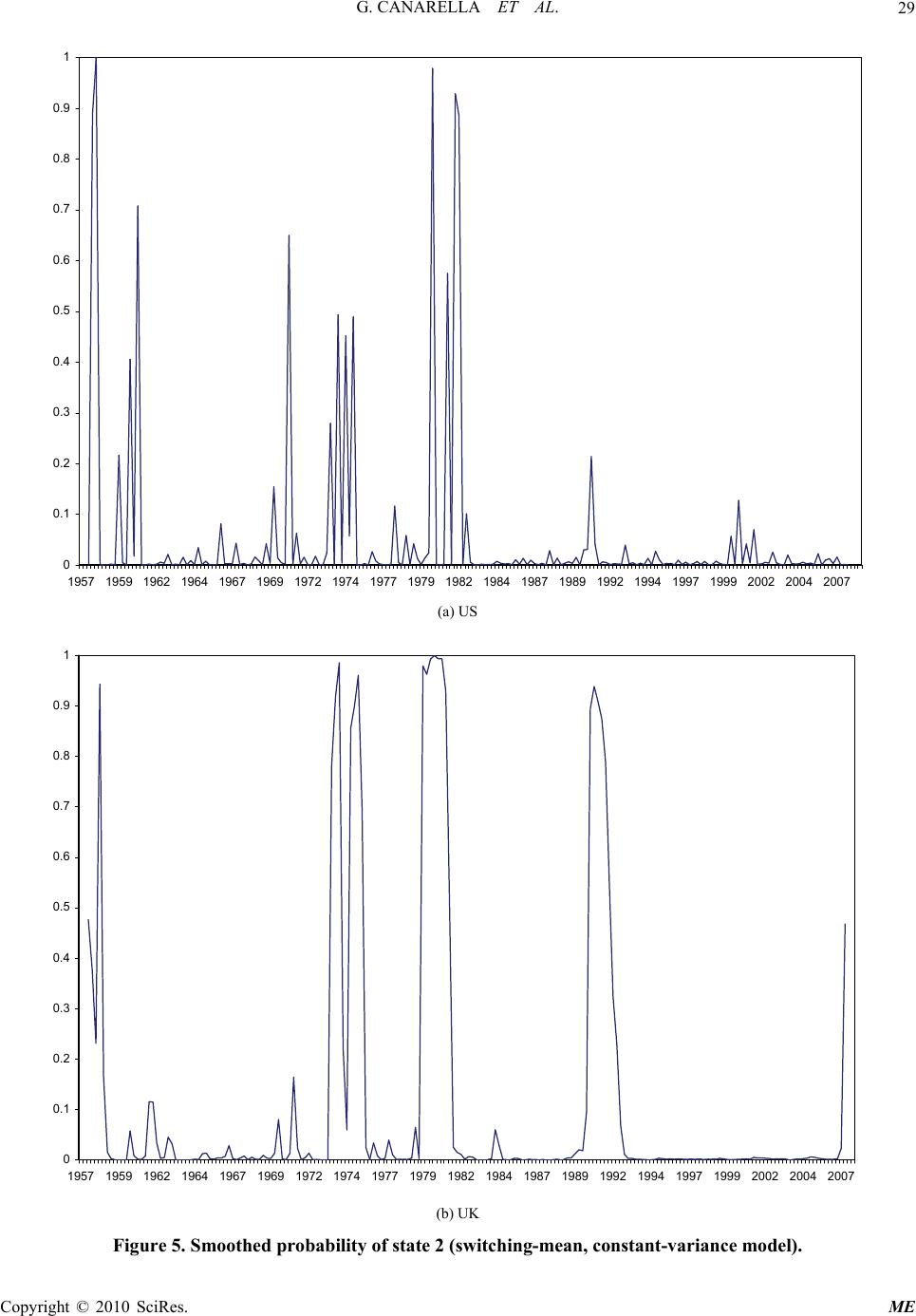

G. CANARELLA ET AL.29
0
0.1
0.2
0.3
0.4
0.5
0.6
0.7
0.8
0.9
1
1957 19591962 1964 1967 1969 1972 1974 19771979 1982 1984 1987 1989 1992 1994 1997 1999 2002 2004 2007
(a) US
0
0.1
0.2
0.3
0.4
0.5
0.6
0.7
0.8
0.9
1
1957 19591962 19641967 1969 19721974 19771979 19821984 19871989 19921994 1997 19992002 20042007
(b) UK
Figure 5. Smoothed probability of state 2 (switching-mean, constant-variance model).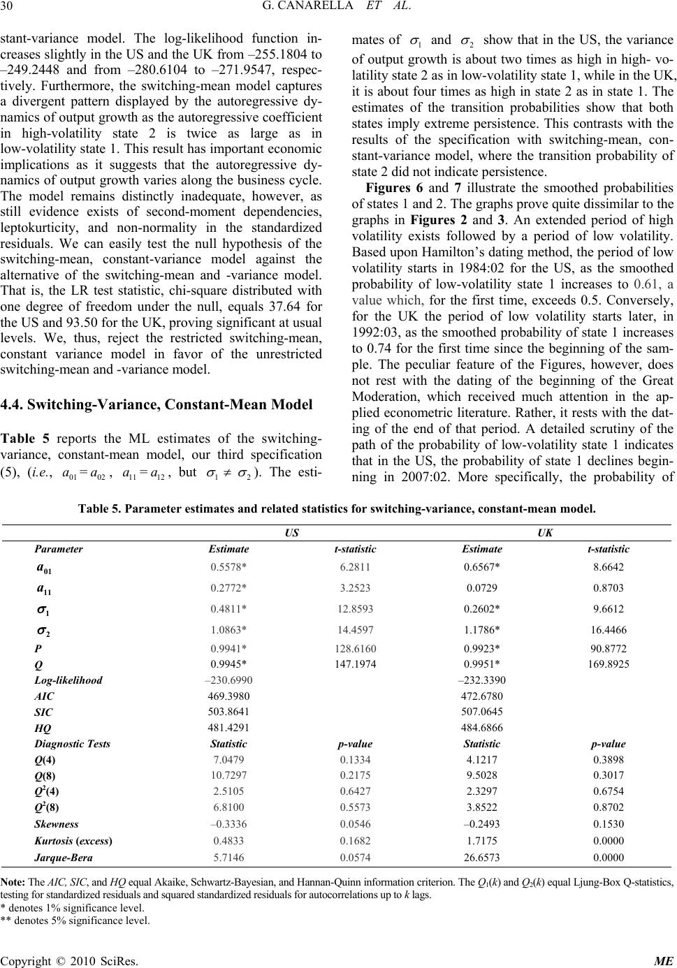

G. CANARELLA ET AL. 30
stant-variance model. The log-likelihood function in-
creases slightly in the US and the UK from –255.1804 to
–249.2448 and from –280.6104 to –271.9547, respec-
tively. Furthermore, the switching-mean model captures
a divergent pattern displayed by the autoregressive dy-
namics of output growth as the autoregressive coefficient
in high-volatility state 2 is twice as large as in
low-volatility state 1. This result has important economic
implications as it suggests that the autoregressive dy-
namics of output growth varies along the business cycle.
The model remains distinctly inadequate, however, as
still evidence exists of second-moment dependencies,
leptokurticity, and non-normality in the standardized
residuals. We can easily test the null hypothesis of the
switching-mean, constant-variance model against the
alternative of the switching-mean and -variance model.
That is, the LR test statistic, chi-square distributed with
one degree of freedom under the null, equals 37.64 for
the US and 93.50 for the UK, proving significant at usual
levels. We, thus, reject the restricted switching-mean,
constant variance model in favor of the unrestricted
switching-mean and -variance model.
4.4. Switching-Variance, Constant-Mean Model
Table 5 reports the ML estimates of the switching-
variance, constant-mean model, our third specification
(5), (i.e., =, =, but
01
a02 a11 a12 a1

2

). The esti-
mates of 1

and 2

show that in the US, the variance
of output growth is about two times as high in high- vo-
latility state 2 as in low-volatility state 1, while in the UK,
it is about four times as high in state 2 as in state 1. The
estimates of the transition probabilities show that both
states imply extreme persistence. This contrasts with the
results of the specification with switching-mean, con-
stant-variance model, where the transition probability of
state 2 did not indicate persistence.
Figures 6 and 7 illustrate the smoothed probabilities
of states 1 and 2. The graphs prove quite dissimilar to the
graphs in Figures 2 and 3. An extended period of high
volatility exists followed by a period of low volatility.
Based upon Hamilton’s dating method, the period of low
volatility starts in 1984:02 for the US, as the smoothed
probability of low-volatility state 1 increases to 0.61, a
value which, for the first time, exceeds 0.5. Conversely,
for the UK the period of low volatility starts later, in
1992:03, as the smoothed probability of state 1 increases
to 0.74 for the first time since the beginning of the sam-
ple. The peculiar feature of the Figures, however, does
not rest with the dating of the beginning of the Great
Moderation, which received much attention in the ap-
plied econometric literature. Rather, it rests with the dat-
ing of the end of that period. A detailed scrutiny of the
path of the probability of low-volatility state 1 indicates
that in the US, the probability of state 1 declines begin-
ning in 2007:02. More specifically, the probability of
Table 5. Parameter estimates and related statistics for switching-variance, constant-mean model.
US UK
Parameter Estimate t-statistic Estimate t-statistic
01
a 0.5578* 6.2811 0.6567* 8.6642
11
a 0.2772* 3.2523 0.0729 0.8703
1

0.4811* 12.8593 0.2602* 9.6612
2

1.0863* 14.4597 1.1786* 16.4466
P 0.9941* 128.6160 0.9923* 90.8772
Q 0.9945* 147.1974 0.9951* 169.8925
Log-likelihood –230.6990 –232.3390
AIC 469.3980 472.6780
SIC 503.8641 507.0645
HQ 481.4291 484.6866
Diagnostic Tests Statistic p-value Statistic p-value
Q(4) 7.0479 0.1334 4.1217 0.3898
Q(8) 10.7297 0.2175 9.5028 0.3017
Q2(4) 2.5105 0.6427 2.3297 0.6754
Q2(8) 6.8100 0.5573 3.8522 0.8702
Skewness –0.3336 0.0546 –0.2493 0.1530
Kurtosis (excess) 0.4833 0.1682 1.7175 0.0000
Jarque-Bera 5.7146 0.0574 26.6573 0.0000
Note: The AIC, SIC, and HQ equal Akaike, Schwartz-Bayesian, and Hannan-Quinn information criterion. The Q1(k) and Q2(k) equal Ljung-Box Q-statistics,
testing for standardized residuals and squared standardized residuals for autocorrelations up to k lags.
* denotes 1% significance level.
** denotes 5% significance level.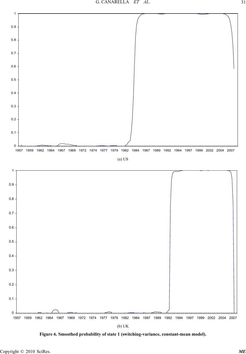

G. CANARELLA ET AL.31
0
0.1
0.2
0.3
0.4
0.5
0.6
0.7
0.8
0.9
1
1957 1959 1962 1964 1967 1969 1972 1974 1977 1979 1982 1984 1987 1989 1992 1994 1997 1999 2002 2004 2007
(a) US
0
0.1
0.2
0.3
0.4
0.5
0.6
0.7
0.8
0.9
1
1957 1959 1962 19641967 1969 1972 1974 1977 19791982 1984 1987 19891992 1994 1997 1999 2002 20042007
(b) UK
Figure 6. Smoothed probability of state 1 (switching-variance, constant-mean model).

G. CANARELLA ET AL. 32
0
0.1
0.2
0.3
0.4
0.5
0.6
0.7
0.8
0.9
1
1957195919621964 196719691972197419771979 19821984 1987198919921994 1997 1999200220042007
(a) US
0
0.1
0.2
0.3
0.4
0.5
0.6
0.7
0.8
0.9
1
195719591962 196419671969 19721974 19771979 1982 19841987 1989199219941997 1999 20022004 2007
(b) UK
Figure 7. Smoothed probability of state 2 (switching-variance, constant-mean model).

G. CANARELLA ET AL. 33
4.5. Regime-Switching Stationarity Tests
low volatility goes from 0.91 in 2007:01 to 0.85 in
2007:02, to 0.75 in 2007:03, and to 0.58 in 2007:04. In
the UK, the evidence that “Great Moderation” ended
appears even more striking. The probability of low vari-
ability in 2006:04 equals 0.94, but in 2007:01 it drops to
0.76, and in 2007:02 to 0.00.
Table 6 reports the estimation results for the switching
regime ADF test (8) for q = 0 (i.e., a switching regime
DF test). Strong evidence emerges to support locally
stationary output growth in both the US and the UK. The
estimates of and both prove negative in the
high and low volatility regimes, and the associated t-
values far exceed in absolute value the Dickey-Fuller
statistics. Note, however, that these t-values do not fol-
low the Dickey-Fuller distribution. In [43] Monte-Carlo
methods are used to calculate the p-values for the
t-statistics. We do not pursue this approach for two rea-
sons. First, we strongly reject the single-regime ADF in
favor of Markov switching ADF. The maximized values
of likelihood function for the single regime ADF equals
–255.18 and –280.61 for the US and the UK, respectively.
Consequently, the LR test statistic equals 51.68 for the
US, while for the UK, it equals 114.48. Thus, we can
clearly reject the null in both cases even after invoking
Davies’ upper bound. Second, both regimes prove locally
stationary, vastly different from the results obtained by
[32]. Furthermore, our main interest lies in dating the
two regimes. From this viewpoint, the results of the
Markov switching ADF regressions corroborate the dat-
ing evidence on the Great Moderation previously ob-
tained. Figures 8 and 9 plot the smoothed probabilities.
11
b12 b
Unlike the switching-mean, constant-variance model,
we cannot reject the restricted switching-variance, con-
stant-mean model in the US case in favor of the unre-
stricted switching-mean and -variance model. The LR
test statistic, chi-square distributed with two degree of
freedom under the null, equals 0.5556, which is not sig-
nificant. In the UK, however, the LR test statistic equals
14.2754, which is significant at usual levels. Thus, we
can reject the switching-mean, constant- variance model
for both the US and the UK in favor of the switch-
ing-mean and -variance model, but we can only reject the
switching-variance, constant-mean only for the UK.
The results of our analysis suggest that the growth of
real GDP for the US and the UK exhibit Markov-
switching behavior. Based on the evidence of a two-state
Markov-switching dynamics, the issue, however, arises
with respect to the stationarity of the two growth-rate
series. According to the single-regime standard ADF test
statistics, the two series prove stationary. The ADF sta-
tistics (with intercept and 0 lags on the differences) equal
–10.53258 and –15.00517, respectively, for the US and
the UK.
Table 6. Parameter estimates and related statistics for the markov-switching unit-root model.
US UK
Parameter Estimate t-statistic Estimate t-statistic
01
a 0.5715* 6.6226 0.2724* 4.7169
02
a 0.5975* 4.5554 0.6951* 6.1209
11
b –0.7633* –7.1754 –0.4037* –5.0967
12
b –0.7008* –7.5390 –1.1131* –13.0996
1

0.4781* 12.4593 0.2758* 12.2513
2

1.0867* 14.0693 1.1697* 17.9006
p 0.9941* 138.5665 0.9932* 115.0833
q 0.9945* 174.948 0.9952* 164.9087
Log-likelihood –229.3400 –223.3798
AIC 470.6801 458.7598
SIC 522.3196 510.2792
HQ 478.6999 466.7569
Diagnostic Tests Statistic p-value Statistic p-value
Q(4) 2.2451 0.6908 6.3642 0.1735
Q(8) 8.1799 0.4161 15.3955 0.0519
Q2(4) 13.7143 0.0083 17.3847 0.0016
Q2(8) 28.3926 0.0004 20.7653 0.0078
Skewness 3.9664 0.0000 0.3083 0.0772
Kurtosis (excess) 19.7141 0.0000 3.7843 0.0000
Jarque-Bera 3800.7748 0.0000 122.5144 0.0000
Note: The AIC, SIC, and HQ equal Akaike, Schwartz-Bayesian, and Hannan-Quinn information criterion. The Q1(k) and Q2(k) equal Ljung-Box Q-statistics,
testing for standardized residuals and squared standardized residuals for autocorrelations up to k lags.
* denotes 1% significance level.
** denotes 5% significance level.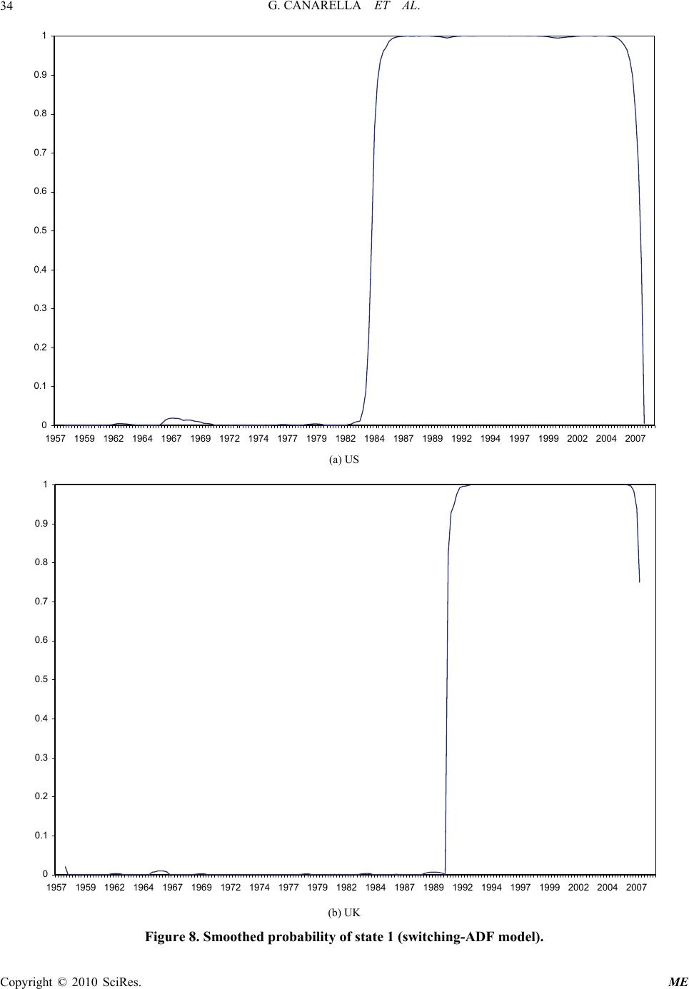

G. CANARELLA ET AL. 34
0
0.1
0.2
0.3
0.4
0.5
0.6
0.7
0.8
0.9
1
1957 195919621964 1967196919721974 1977 197919821984198719891992199419971999200220042007
(a) US
0
0.1
0.2
0.3
0.4
0.5
0.6
0.7
0.8
0.9
1
1957 1959196219641967196919721974 19771979 1982198419871989 1992 19941997199920022004 2007
(b) UK
Figure 8. Smoothed probability of state 1 (switching-ADF model).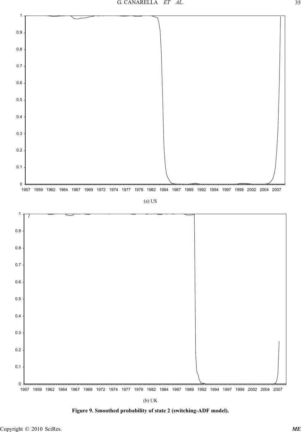

G. CANARELLA ET AL.35
0
0.1
0.2
0.3
0.4
0.5
0.6
0.7
0.8
0.9
1
1957 19591962 19641967 196919721974 1977197919821984 1987198919921994 199719992002 20042007
(a) US
0
0.1
0.2
0.3
0.4
0.5
0.6
0.7
0.8
0.9
1
1957 195919621964 196719691972197419771979198219841987198919921994 1997 1999200220042007
(b) UK
Figure 9. Smoothed probability of state 2 (switching-ADF model).

G. CANARELLA ET AL. 36
each regime and allow the conditional variances to fol-
low a switching ARCH (2) process-SWARCH(2), our
fifth specification (9). We use the AIC criterion to
choose the SWARCH (2) structure. Table 7 reports the
estimates for the single-regime version of the model. The
autoregressive parameters nearly match those reported
for the constant variance regime-switching model. The
conditional-variance parameters prove statistically sig-
nificant, as expected. For the US, however, the sum of
the ARCH estimates + falls significantly below
unity, which satisfies the stationarity assumption. Con-
versely, for the UK, a Wald test supports the violation of
the stationarity assumption, whereby the conditional va-
riance follows an integrated ARCH and + = 1.
The Wald test statistic, distributed chi-square(1) under
the null, equals 0.066, which proves insignificant at any
usual level (p-value = 0.7971).
1
b2 b
1
b2 b
They also show ample evidence for regime changes in
the real GDP growth rate. Such changing-persistence
behavior would not emerge from the standard unit-root
tests, which assume persistence remains constant through
the sample sub-periods.
The dates of the beginning and ending of the Great
Moderation nearly match those obtained using the Mar-
kov-switching models. Based upon Hamilton’s dating
method, the period of low volatility starts for the US in
1984:03, as the smoothed probability of state 1 increases
to 0.76 and ends in 2007:03 as the smoothed probability
of low variability decreases to 0.41. This decline is im-
mediately followed in 2007:04 by a further sharp de-
crease to 0.0052. For the UK, instead, the dates of the
beginning and ending of the Great Moderation are
slightly different from the ones detected by the Markov-
switching model. The Markov switching ADF regression
places the beginning of the Great Moderation on the last
quarter of 1990 rather than the third quarter of 1992. The
Markov-switching ADF regression does not date the end
of the Great Moderation in the UK, but hints at it, as the
probability of low variability declines from 0.94 in
2007:01 to 0.74 in 2007:02.
Table 8 reports estimates of the regime-switching AR
(1)-ARCH (2) model. Results remain virtually un-
changed for higher ARCH (3) or lower ARCH (1) lags of
the ARCH process. The striking feature of the results
suggests that although the states remain highly persistent,
the underlying fundamental ARCH (2) process does not.
That is, the volatility effects as revealed by the switching
ARCH estimates do not exhibit high persistence. This
reflects the estimates of the decay parameter,

=
+ of the ARCH processes. The volatility effects for
1
b
2
b
4.6. Autoregressive Conditional Heteroskedastic
Variance Markov Regime-Switching Model
We now relax the assumption of constant variance within
Table 7. Parameter estimates and related statistics for the single-regime, AR (1)-ARCH (2) model.
US UK
Parameter Estimate t-statistic Estimate t-statistic
0
a 0.5969* 7.1186 0.5854* 6.7926
1
a 0.3307* 4.7919 0.1393 1.2009
0
b 0.2955* 4.8300 0.2858* 4.3675
1
b 0.2249* 2.6940 0.5764* 3.2228
2
b 0.4765* 3.2284 0.4802** 2.2408
Log-likelihood –240.7973 –261.8643
AIC 491.5946 533.7286
SIC 534.6772 576.7117
HQ 501.6257 543.7372
Diagnostic Tests Statistic p-value Statistic p-value
Q1(4) 8.2489 0.0829 7.4829 0.1125
Q1(8) 12.6372 0.1250 18.1080 0.0204
Q2(4) 5.1937 0.2680 3.4514 0.4853
Q2(8) 14.3546 0.0730 11.2561 0.1876
Skewness –0.1916 0.2696 0.0484 0.7813
Kurtosis (excess) 1.3780 0.0000 3.6587 0.0000
Jarque-Bera 17.2194 0.0001 111.6327 0.0000
Note: The AIC, SIC, and HQ equal Akaike, Schwartz-Bayesian, and Hannan-Quinn information criterion. The Q1(k) and Q2(k) equal Ljung-Box
Q-statistics, testing for standardized residuals and squared standardized residuals for autocorrelations up to k lags.
* denotes 1% significance level.
** denotes 5% significance level.

G. CANARELLA ET AL.37
Table 8. Parameter estimates and related statistics for the markov regime-switching AR (1)-ARCH (2) model.
US UK
Parameter Estimate t-statistic Estimate t-statistic
0
a
a
0.5663* 7.0196 0.6320* 10.0572
1
b
0.3050* 3.9860 0.0960 1.1875
0
b
0.1775* 3.8577 0.0433* 2.9659
1
b
0.0741 0.8184 0.2324 1.8457
2
p
0.1666 1.1977 0.1504 1.3099
0.9942* 68.7670 0.9919* 33.9063
q 0.9945* 108.7333 0.9948* 226.9010
2

5.2573* 3.5984 22.3155* 3.3458
Log-likelihood –228.8731 –228.7725
AIC 469.7462 469.5451
SIC 521.4454 521.1248
HQ 477.7773 477.5536
Diagnostic Tests Statistic p-value Statistic p-value
Q1(4) 7.3931 0.1165 4.4542 0.3480
Q1(8) 10.5687 0.2274 11.3292 0.1837
Q2(4) 1.2823 0.8644 2.4926 0.6460
Q2(8) 7.9561 0.4378 3.9427 0.8622
Skewness –0.1409 0.4167 0.1413 0.4179
Kurtosis (excess) 0.2589 0.4602 2.0608 0.0000
Jarque-Bera 1.2338 0.5396 36.0588 0.0000
Note: The AIC, SIC, and HQ equal Akaike, Schwartz-Bayesian, and Hannan-Quinn information criterion. The Q1(k) and Q2(k) equal Ljung-Box Q-statistics,
testing for standardized residuals and squared standardized residuals for autocorrelations up to k lags.
* denotes 1% significance level.
** denotes 5% significance level.
the US switching ARCH model die out in about 3 quar-
ters (), while those of the single-regime
ARCH model persist for more than three years
(). Conversely, the volatility effects for the
UK switching ARCH model die out in about 4 quarters
().
30.0139
 
0.0141
0.0214
12

4
 
We note, however, that the ARCH terms in the single-
regime model prove highly significant while in the
switching-regime model, they lose their significance. In
the switching-ARCH model of (9), changes in the regime
do not affect the dynamics of the process, just the scale
[31,54,55], which reflects the 2

parameter. The esti-
mates of this parameter indicate that for the UK, the
conditional variance in the high volatility state exceeds
the low-volatility state by more than 22 times. For the
US, instead, this ratio equals about 5. The residual diag-
nostics clearly indicate that no evidence exists of second-
moment nonlinear dependencies in the standardized re-
siduals.
In fact, the autoregressive coefficients for the ARCH(2)
models in both regimes prove insignificantly different
from zero. This suggests a homoskedastic error process,
which matches the findings of [6]. They report that the
GARCH and ARCH processes disappear once dummy
variables capture the shift from high to low-volatility
regimes.
A LR test rejects the single-regime constant-variance
model in favor of the single-regime ARCH model. The
LR test statistic, distributed as chi-squared with two de-
grees of freedom under the null, equals 28.7662 in the
US and 37.4922 in the UK, which proves significant at
any usual level. The regime-switching AR(1)-ARCH(2)
model yields significantly higher log likelihood values
than the single-regime AR(1)-ARCH(2). So, we unam-
biguously reject the null of no Markov switching by the
Davies upper-bound test. The LR test statistics, distrib-
uted as chi-squared with one degree of freedom under the
null, equal 23.8484 and 66.1836 for the US and the UK,
respectively. These values, even after invoking Davies’s
upper-bound adjustment, prove highly significant. Thus,
while the application of the single-regime ARCH model
leads to nearly non-stationary variance processes, the use
of the Markov-switching ARCH model substantially
improves the results.
The results of the SWARCH model further confirm
the previous dates of the beginning and end of the Great
Moderation. The smoothed probabilities for the low- and
high-volatility regimes (states 1 and 2, respectively) fol-
low very closely the results found without the ARCH
component. Figures 10 and 11 illustrate this point.
Based on Hamilton’s dating method, the switching-
ARCH model captures reasonably well the period of the
Great Moderation. The low-volatility regime starts in the
S in 1984:02, as the smoothed probability increases to U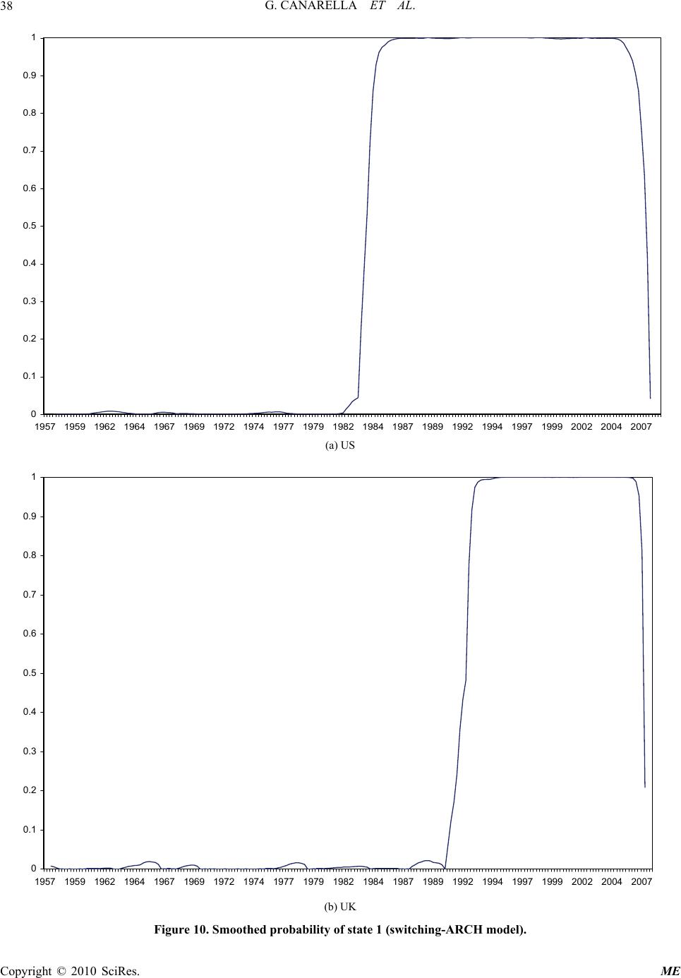

G. CANARELLA ET AL. 38
0
0.1
0.2
0.3
0.4
0.5
0.6
0.7
0.8
0.9
1
1957 195919621964196719691972197419771979 1982198419871989199219941997 1999200220042007
(a) US
0
0.1
0.2
0.3
0.4
0.5
0.6
0.7
0.8
0.9
1
1957 1959 19621964 1967 1969 1972 1974 1977 1979 1982 1984 19871989 1992 1994 1997 19992002 2004 2007
(b) UK
Figure 10. Smoothed probability of state 1 (switching-ARCH model).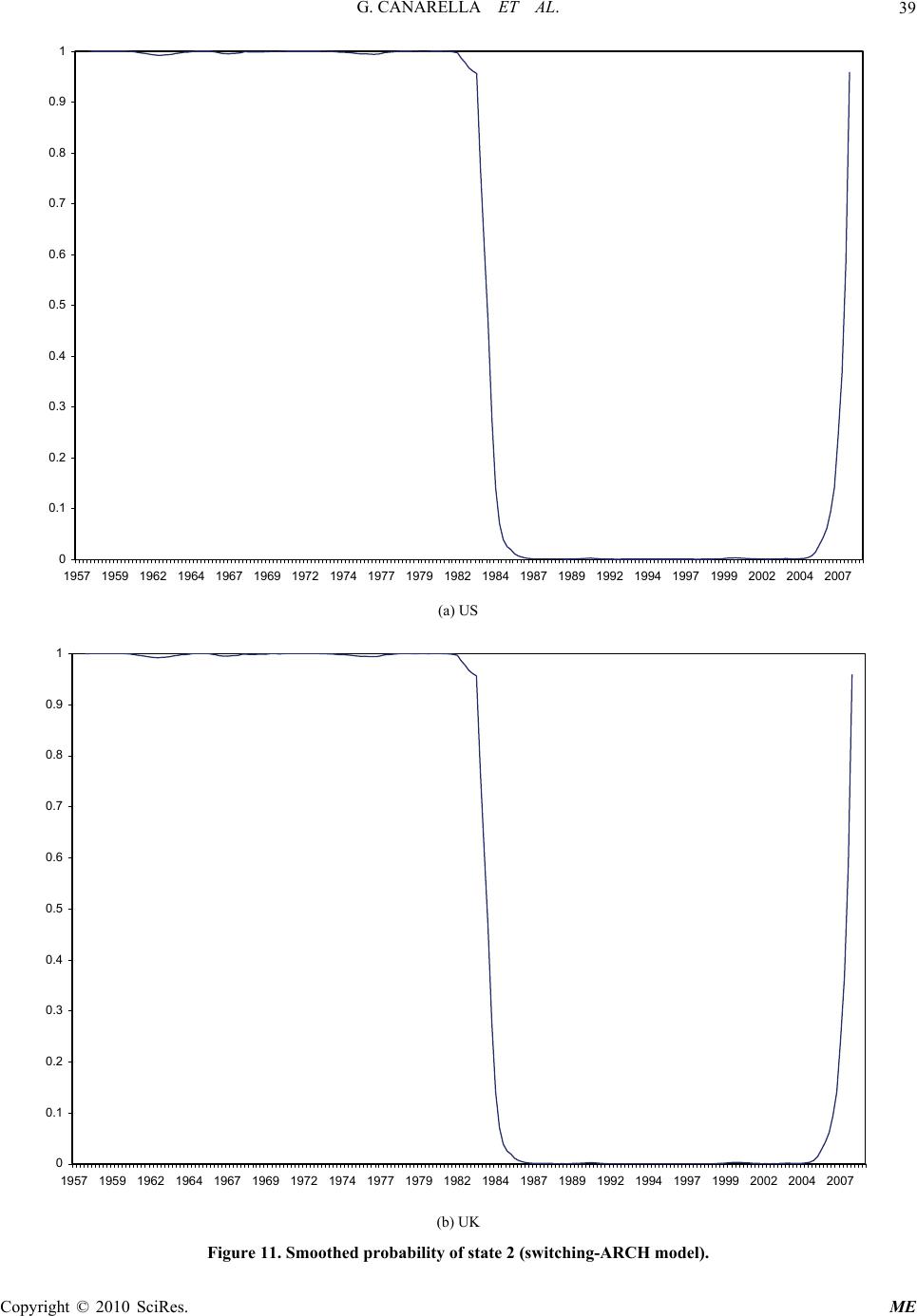

G. CANARELLA ET AL.39
0
0.1
0.2
0.3
0.4
0.5
0.6
0.7
0.8
0.9
1
1957 1959 196219641967 1969 197219741977 1979 198219841987 1989 199219941997 1999 200220042007
(a) US
0
0.1
0.2
0.3
0.4
0.5
0.6
0.7
0.8
0.9
1
1957 1959 1962 196419671969 19721974 19771979 198219841987 198919921994 1997 1999200220042007
(b) UK
Figure 11. Smoothed probability of state 2 (switching-ARCH model).

G. CANARELLA ET AL. 40
0.72, and ends in 2007:03, as the smoothed probability of
low variability decreases to 0.41. This decline is imme-
diately followed in 2007:04 by a further sharp decrease
to 0.0414. Similarly, for the UK, the low-volatility re-
gime starts in 1992:03, as the smoothed probability rises
to 0.77 and ends in 2007:02 as the smoothed probability
of low-variability declines to 0.20.
5. Conclusions
The Great Moderation, the significant decline in the va-
riability of economic activity, provides a most remark-
able feature of the macroeconomic landscape in the last
twenty years. A number of papers document the begin-
ning of the Great Moderation in the US and the UK (e.g.,
[11-17]). In this paper, we use the Markov regime-
switching models of [10] and [31] to document the end
of the Great Moderation. The analysis uses quarterly
rates of growth of real GDP from 1957:02 to 2007:04 for
the US and from 1957:02 to 2007:02 for the UK. Our
results place the end of the Great Moderation in 2007.
The Great Moderation in the US and the UK begin at
different point in time. In the US the Great Moderation
starts in 1983. In the UK, instead, it begins almost 10
years later.5 The explanations for the Great Moderation
fall into generally three different categories—good mon-
etary policy, improved inventory management, or good
luck. According to [16], a combination of good monetary
policy and better inventory management led to the Great
Moderation.
The end of the Great Moderation, however, occurs at
approximately the same time in both the US and the UK.
The end of the Great Moderation may reflect different
reasons, and one may conjecture about reasons for the
end. It seems unlikely that good monetary policy would
turn into bad policy or that better inventory management
would turn into worse management. Rather, the likely
explanation comes from bad luck. Two likely culprits
exist—energy price and housing price shocks.6 We leave
this conjecture about the end of the Great Moderation for
future research as more data become available with
which to address the question.
Relating directly to the comments in the prior para-
graph, Reference [56] compares the current sub-prime
crisis in the US to 18 bank-centered financial crises.
Striking similarities exist between the current US situa-
tion and those of the 18 financial crises examined, in-
cluding the run up and collapse of housing and equity
prices, the current level of the current account deficit to
GDP, the pattern of changes in real GDP per capita
growth, and the rise in the public debt’s share of GDP.
They also state that a similar situation exists in the UK.
In sum, the US situation, and the situation in the UK,
provide “stunning quantitative and qualitative parallels
across a number of standard financial crisis indicators.”
Besides the Great Moderation issue, another reason
exists to investigate regime changes in the volatility of
economic activity. The well-known autoregressive con-
ditionally heteroskedastic models, based on the seminal
work by [1] and [2], play an important role in the estima-
tion of volatilities. Problems associated with estimating
such models, however, may arise if the underlying vola-
tility process incorporates structural breaks, especially
shifts in the overall level of volatility.7 In this paper, we
show that the variance process is (almost) non-stationary.
The high persistence that we find in single-regime mod-
els may merely reflect the disregarding the problem of
regime changes (i.e., the high persistence may simply
occur because of a misspecified model). We find persis-
tence. The persistence, however, does not reside in the
shocks, but rather in the regimes.
We must confess in conclusion that we did not expect
our finding of the possible end to the Great Moderation.
That finding came as a complete surprise. Is it true?
Time will tell. Before concluding, we offer some caveats
about our finding. First, the reliability of our data series
probably deteriorates at the end of the sample, where
data revisions may still occur. Such data revisions could
reverse our finding. Second, if the Great Moderation
largely reflects better monetary policy, then will not the
central banks engage in the appropriate actions that will
lead to a false signal? That is, will monetary policy mak-
ers neutralize those factors that signal a return to the high
volatility regime? Third, the added worldwide demand
coming from China, India, and other countries may con-
stitute an added dose of “bad luck,” especially when
combined with the energy and housing market shocks. In
sum, we conclude that the empirical evidence signals the
end of the Great Moderation. Nonetheless, we still carry
some reservations about our finding.
5Our findings on the beginning of the Great Moderation, using different
methodologies, match those reported in [20]. The methodology em-
p
loyed by [6], however, cannot identify the end of the Great Modera-
tion, except with the passage of time.
6The reasons why the effects of oil price shocks differ so much be-
tween the 1970s and the 2000s are considered by [13], using data
through 2005: 4. According to [13] four different factors help to ex-
p
lain the differences -“(a) good luck (i.e., lack of concurrent adverse
shocks), (b) smaller share of oil in production, (c) more flexible labor
markets, and (d) improvements in monetary policy.” (p. 1). We note
that since 2005:4, the oil price shock worsened dramatically and the
housing market crisis in the US and the UK appeared, another concur-
rent adverse shock.
7In this regard, our findings confirm those of [6], who use a different
methodology. They find that introducing dummy variables to capture
the regime switches in the volatility of real GDP growth eliminates the
GARCH and ARCH processes for the volatility processes in each sub-
p
eriod. Table 8 reports similar results in that the autoregressive coeffi-
cients in the ARCH (2) processes in the Markov regime-switching AR
(1)-ARCH (2) model prove insignificantly different from zero. In other
words, a homoskedastic error process exists for the high-and low-
volatility regimes.

G. CANARELLA ET AL.41
6
. References
[1] R. F. Engle, “Autoregressive Conditional Heteroscedasticity
with Estimates of the Variance of United Kingdom
Inflation,” Econometrica, Vol. 50, No. 4, 1982, pp. 987-
1007.
[2] T. Bollerslev, “Generalized Autoregressive Conditional
Heteroskedasticity,” Journal of Econometrics, Vol. 31,
No. 3, 1986, pp. 307-327.
[3] Klaassen, “Improving GARCH Volatility Forecasts with
Regime-Switching GARCH,” Empirical Economics, Vol.
27, No. 2, 2002, pp. 363-394.
[4] C. G. Lamoureux and W. D. Lastrapes, “Persistence in
Variance, Structural Change and the GARCH Model,”
Journal of Business and Economic Statistics, Vol. 8, No.
2, 1990, pp. 225-234.
[5] A. Timmerman, “Moments of Markov Switching Models,”
Journal of Econometrics, Vol. 96, No. 1, 2000, pp. 75-
111.
[6] W. Fang, S. M. Miller and C. Lee, “Cross-Country
Evidence on Output Growth Volatility: Nonstationary
Variance and GARCH Models,” Scottish Journal of
Political Economy, Vol. 55, No. 4, 2008, pp. 509-541.
[7] A. Sansó, V. Arragó and J. L. Carrion, “Testing for
Change in the Unconditional Variance of Financial Time
Series,” Revista de Economiá Financiera, Vol. 4, No. 4,
2004, pp. 32-53.
[8] W. Fang and S. M. Miller, “The Great Moderation and
the Relationship between Output Growth and its
Volatility,” Southern Economic Journal, Vol. 74, No. 3,
2008, pp. 819-838.
[9] J. D. Hamilton, “Rational-Expectations Econometric
Analysis of Changes in Regime: An Investigation of the
Term Structure of Interest Rates,” Journal of Economic
Dynamics and Control, Vol. 12, No. 2-3, 1988, pp. 385-
423.
[10] J. D. Hamilton, “A New Approach to the Economic
Analysis of Nonstationary Time Series and the Business
Cycle,” Econometrica, Vol. 57, No. 2, 1989, pp. 357-384.
[11] J. Kim and C. R. Nelson, “Has the U.S. Economy
Become More Stable? A Bayesian Approach Based on a
Markov-Switching Model of the Business Cycle,” Review
of Economics and Statistics, Vol. 81, No. 4, 1999, pp.
608-616.
[12] M. M. McConnell and G. Perez-Quiros, “Output Fluctua-
tions in the United States: What has Changed since the
Early 1980’s?” American Economic Review, Vol. 90, No.
5, 2000, pp. 1464-1476.
[13] O. J. Blanchard and J. Galí, “The Macroeconomic Effects
of Oil Price Shocks: Why are the 2000s So Different
from the 1970s?” MIT Department of Economics
Working Paper No. 07-21, 2007.
[14] O. J. Blanchard and J. Simon, “The Long and Large
Decline in U. S. Output Volatility,” Brookings Papers on
Economic Activity, Vol. 2001, No. 1, 2001, pp. 135-164.
[15] T. C. Mills and P. Wang, “Have Output Growth Rates
Stabilized? Evidence from the G-7 Economies,” Scottish
Journal of Political Economy, Vol. 50, No. 3, 2003, pp.
232-246.
[16] P. M. Summers, “What Caused the Great Moderation?
Some Cross-Country Evidence,” Economic Review,
Federal Reserve Bank of Kansas City, 2005, pp. 5-32.
[17] J. H. Stock and M. W. Watson, “Understanding Changes
in International Business Cycle Dynamics,” Journal of
the European Economic Association, Vol. 3, No. 5, 2005,
pp. 968-1006.
[18] C. Kent, K. Smith and J. Holloway, “Declining Output
Volatility: What Role for Structural Change?” In: C. Kent
and D. Norman, Eds., The Changing Nature of the
Business Cycle, Reserve Bank of Australia, 2005, pp.
146-180.
[19] S. G. Cecchetti, A. Flores-Lagunes and S. Krause,
“Assessing the Sources of Changes in the Volatility of
Real Growth,” In: C. Kent and D. Norman, Eds., The
Changing Nature of the Business Cycle, Reserve Bank of
Australia, 2005, pp. 115-138.
[20] J. H. Stock and M. W. Watson, “Has the Business Cycle
Changed? Evidence and Explanations,” Monetary Policy
and Uncertainty: Adapting to a Changing Economy,
Proceedings of Symposium sponsored by Federal Reserve
Bank of Kansas City, Jackson Hole, Wyoming, 2003, pp.
9-56.
[21] S. Ahmed, A. Levin and B. A. Wilson, “Recent U.S.
Macroeconomic Stability: Good Policies, Good Practices,
or Good Luck?” Review of Economics and Statistics, Vol.
86, No. 3, 2004, pp. 824-832.
[22] R. Clarida, J. Galí and M. Gertler, “Monetary Policy
Rules and Macroeconomic Stability: Evidence and Some
Theory,” Quarterly Journal of Economics, Vol. 115, No.
1, 2000, pp. 147-180.
[23] B. S. Bernanke, “The Great Moderation,” Speech at Eas-
tern Economic Association, Washington, February 20
2004.
[24] J. H. Stock and M. W. Watson, “Has the Business Cycle
Changed and Why?” In: M. Gertler and K. Rogoff, Eds.,
NBER Macroannual 2002, MIT Press, Cambridge, 2002,
pp. 159-218.
[25] G. E. Primiceri, “Time Varying Structural Vector Autore-
Gressions and Monetary Policy,” Review of Economic
Studies, Vol. 72, No. 3, 2005, pp. 821-852.
[26] C. Sims and T. Zha, “Were There Regime Switches in U.S.
Monetary Policy?” American Economic Review, Vol. 96,
No. 1, 2006, pp. 54-81.
[27] L. Gambetti, E. Pappa and F. Canova, “The Structural
Dynamics of US Output and Inflation: What Explains the
Changes?” Journal of Money, Credit and Banking, Vol.
40, No. 2-3, 2006, pp. 369-388.
[28] T. Lubik and F. Schorfheide, “Testing for Indeterminacy:
An Application to U. S. Monetary Policy,” American
Economic Review, Vol. 94, No. 1, 2004, pp. 190-217.
[29] J. Boivin and M. Giannoni, “Has Monetary Policy
Become More Effective?” The Review of Economics and
Statistics, Vol. 88, No. 3, 2006, pp. 445-462.
[30] L. Benati and P. Surico, “VAR Analysis and the Great

G. CANARELLA ET AL. 42
Moderation, European Central Bank,” Working Paper #
866, February 2008.
[31] J. D. Hamilton and R. Susmel, “Autoregressive Condi-
Tional Heteroskedasticity and Changes in Regime,”
Journal of Econometrics, Vol. 64, No. 1-2, 1994, pp.
307-333.
[32] J. Kim, C. R. Nelson and R. Startz, “Testing for Mean
Reversion in Heteroskedastic Data Based on Gibbs
Sampling Augmented Randomization,” Journal of Empir-
ical Finance, Vol. 5, No. 2, 1998, pp. 131-154.
[33] R. Bhar and S. Hamori, “Alternative Characterization of
the Volatility in the Growth Rate of Real GDP,” Japan
and the World Economy, Vol. 15, No. 2, 2003, pp. 223-
231.
[34] F. X. Diebold, “Comments on Modelling the Persistence
of Conditional Variance,” Econometric Reviews, Vol. 5,
No. 1, 1986, pp. 51-56.
[35] R. F. Engle and T. Bollerslev, “Modelling the Persistence
of Conditional Variance,” Econometric Reviews, Vol. 5,
No. 1, 1986, pp. 1-50.
[36] T. Mikosch and C. Stărică, “Non-Stationarities in Financial
Time Series, the Long-Range Dependence, and the
IGARCH Effects,” Review of Economics and Statistics,
Vol. 86, No. 1, 2004, pp. 378-390.
[37] E. Hillebrand, “Neglecting Parameter Changes in
GARCH Models,” Journal of Econometrics, Vol. 129,
No. 1-2, 2005, pp. 121-138.
[38] W. Kramer and B. T. Azamo, “Structural Change and
Estimated Persistence in the GARCH(1,1)-Model,”
Economics Letters, Vol. 97, No. 1, 2007, pp. 17-23.
[39] S. Gray, “Modeling the Conditional Distribution of
Interest Rates as a Regime Switching Process,” Journal
of Financial Economics, Vol. 42, No. 1, 1996, pp. 27-62.
[40] M. Sola and A. G. Timmerman, “Fitting the Moments: A
Comparison of ARCH and Regime-Switching Models for
Daily Stock Returns,” Working Paper, London Business
School, 1994.
[41] R. Fletcher, “A New Approach to Variable Metric
Algorithm,” Computer Journal, Vol. 13, No. 3, 1970, pp.
317-322.
[42] R. B. Davies, “Hypothesis Testing when a Nuisance
Para-Meter is Present Only under the Alternative,”
Biometrika, Vol. 74, No. 1, 1987, pp. 33-43.
[43] Kanas and M. Genius, “Regime (Non)Stationarity in the
US/UK Real Exchange Rate,” Economics Letters, Vol. 87,
No. 3, 2005, pp. 407-413.
[44] L. Ramchand and R. Susmel, “Cross Correlations across
Major International Markets,” Journal of Empirical
Finance, Vol. 5, No. 4, 1998, pp. 397-416.
[45] C. G. Broyden, “The Convergence of a Class of Double-
Rank Minimization Algorithms,” IMA Journal of Applied
Mathematics, Vol. 6, No. 1, 1970, pp. 76-90.
[46] D. Goldfarb, “A Family of Variable Metric Methods
Derived by Variational Means,” Mathematical Computa-
tion, Vol. 24, 1970, pp. 23-26.
[47] D. F. Shanno, “Conditioning of Quasi-Newton Methods
for Function Minimization,” Mathematics of Computa-
tion, Vol. 24, No. 111, 1970, pp. 647-656.
[48] E. K. Berndt, B. H. Hall, R. E. Hall and J. A. Hausmann,
“Estimation and Inference in Nonlinear Structural
Models,” Annals of Economic and Social Measurement,
Vol. 3, No. 4, 1974, pp. 653-665.
[49] D. Brunner, “Conditional Asymmetries in Real GDP: A
Semiparametric Approach,” Journal of Business and
Economic Statistics, Vol. 10, No. 1, 1992, pp. 65-72.
[50] D. Brunner, “On the Dynamic Properties of Asymmetric
Models of Real GDP,” The Review of Economics and
Statistics, Vol. 79, No. 2, 1997, pp. 321-326.
[51] M. V. French and D. Sichel, “Cyclical Patterns in the
Variance of Economic Activity,” Journal of Business and
Economic Statistics, Vol. 11, No. 1, 1993, pp. 113-119.
[52] B. E. Hansen, “The Likelihood Ratio Test Under Non-
standard Conditions: Testing the Markov Switching
Model of GNP,” Journal of Applied Econometrics, Vol. 7,
1992, pp. S61-S82.
[53] R. Garcia, “Asymptotic Null Distribution of the Likeli-
hood Ratio Test in Markov Switching Models,” Interna-
tional Economic Review, Vol. 39, No. 3, 1998, pp. 763-
788.
[54] M. Liu, “Modelling Long Memory in Stock Market
Volatility,” Journal of Econometrics, Vol. 99, No. 1,
2000, pp. 139-171.
[55] C. S. Wong and W. K. Li, “On a Mixture Autoregressive
Conditional Heteroskedastic Model,” Journal of the
American Statistical Association, Vol. 96, No. 455, 2001,
pp. 982-995.
[56] C. M. Reinhart and K. S. Rogoff, “Is the 2007 US Sub-
Prime Financial Crisis So Different? An International
Historical Comparison,” American Economic Review:
Papers and Proceedings, Vol. 98, No. 2, 2008, pp. 339-
344.
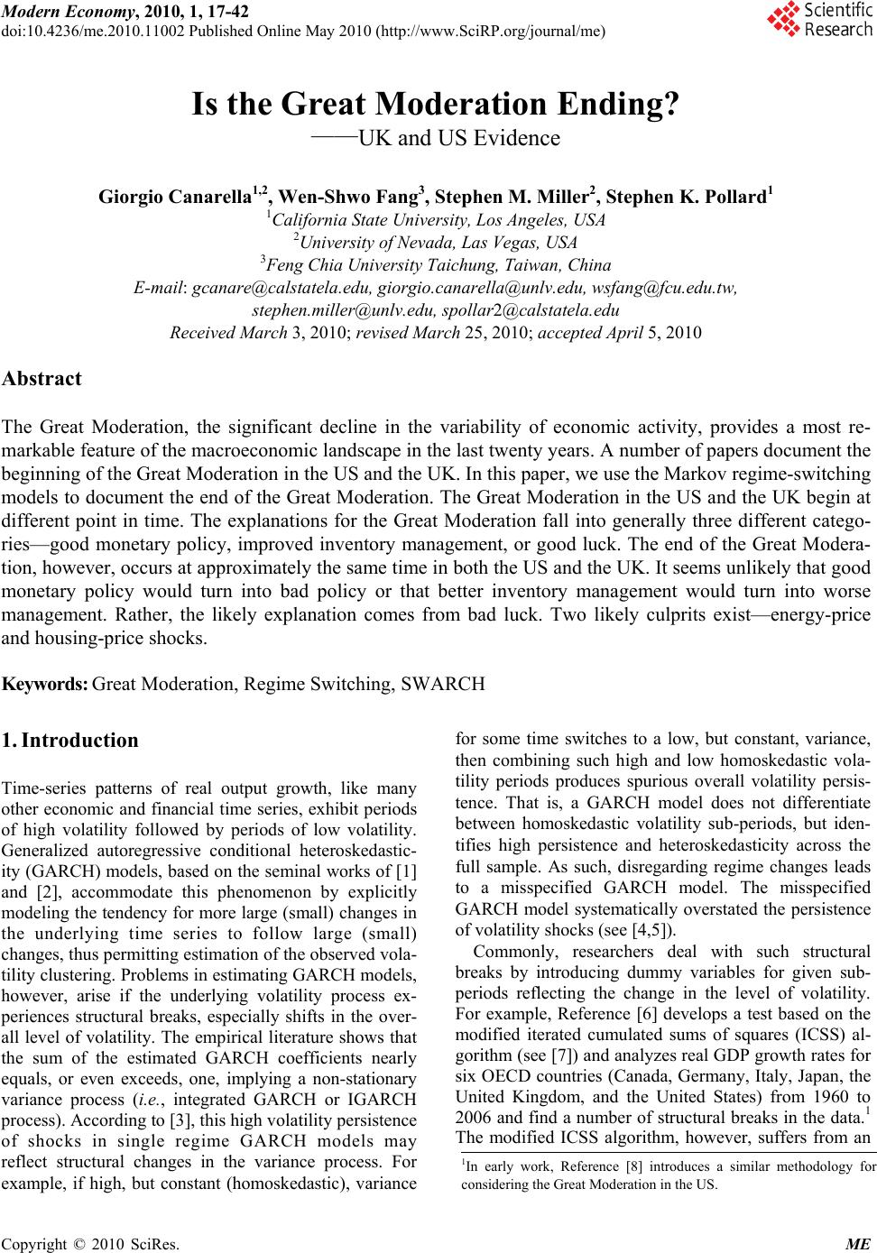