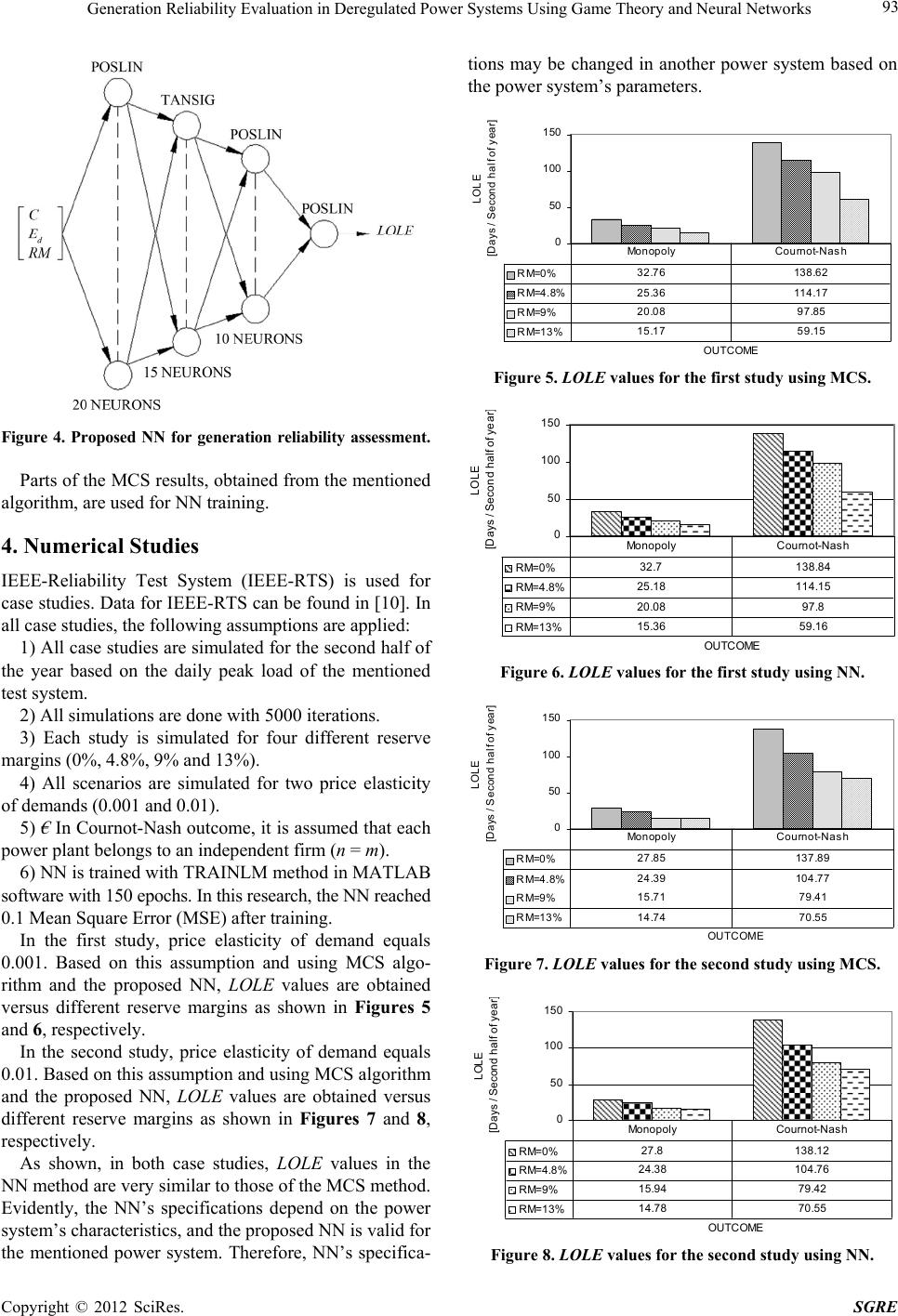
Generation Reliability Evaluation in Deregulated Power Systems Using Game Theory and Neural Networks
Copyright © 2012 SciRes. SGRE
94
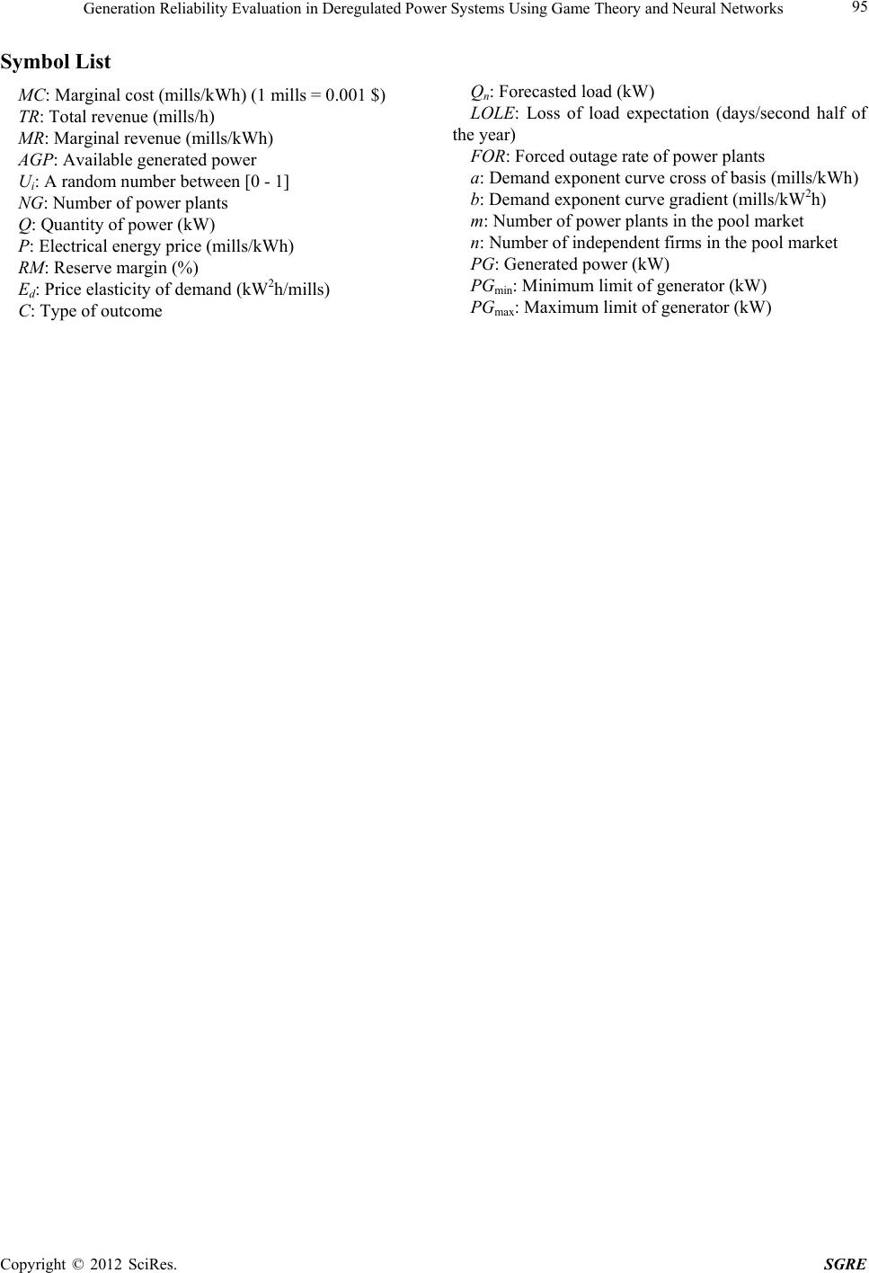
In both case studies, if reserve margin increases, LOLE
will decrease and reliability will improve.
In monopoly market, if price elasticity increases, MR
curve takes less gradient. As a result, intersection of the
power plants’ total offer curve and MR curve occurs at
less demand. This leads to the operation of fewer power
plants. Therefore, in all case studies in monopoly market,
if price elasticity increases, LOLE will decrease.
In Cournot-Nash equilibrium, if price elasticity varies,
the generated power of every power plant varies, too.
Therefore, LOLE will differ based on the share of every
plant’s generated power and FOR.
LOLE values in Cournot-Nash outcome are very big-
ger than those of the monopoly outcome. Because in mo-
nopoly market, only the plants, which are selected by in-
tersection of the total offer and MR curves, are in service
(considering RM), while in Cournot-Nash outcome, all of
the players participate in the market, and the load feeds
based on the plants’ optimum generated power. Therefore,
in monopoly market, at every time period, only a few
plants are in service, while in Cournot-Nash ou tcome, all
of the power plants are in service based on their optimum
generation. Since the number of in-service plants in
Cournot-Nash outcome is very bigger than in monopoly
market, generation reliability in monopoly market is bet-
ter than in Cournot-Nash outcome.
It is worth noting that, since available capacity of hy-
dro plants in IEEE-RTS are different in the first and the
second halves of the year, therefore, in the present work,
simulations were done for the second half of the year.
Evidently, the proposed method can be utilized for every
simulation time.
5. Conclusions
This research deals with generation reliability assessment
in power pool market using GT. Due to the stochastic
behavior of market and generators’ FOR, MCS was used
for simulations. Also, for creation of a unique structure
for reliability assessment, a NN was used, which its out-
puts were very similar to the MCS results.
Based on the players’ cooperation conditions, two out-
comes (Monopoly and Cournot-Nash equilibrium) were
considered. LOLE was used as generation reliability in-
dex, and it was shown that generation reliability in mo-
nopoly market is better than Cournot-Nash model.
Also, in monopoly market, if price elasticity increases,
LOLE will improve. On the other hand , in Cournot-Nash
model, if the price elasticity of demand varies, the power
plants’ generated powers will vary too, and that is why
LOLE changes.
REFERENCES
[1] R. Billinton and R. Allan, “Relia bility Evaluation of Power
Systems,” 2nd Edition, Plenum Press, New York, 1996,
pp. 1, 10, 372.
[2] L. Salvaderi, “Electric Sector Restructuring in Italy,” IEEE
Power Engineering Review, Vol. 20, No. 4, 2000, pp. 12-
16. doi:10.1109/39.833009
[3] H. B. Puttgen, D. R. Volzka and M. I. Olken, “Restructur-
ing and Reregulation of The US Electric Utility Industry,”
IEEE Power Engineering Review, Vol. 21, No. 2, 2001,
pp. 8-10. doi:10.1109/39.896811
[4] R. Azami, A. H. Abbasi, J. Shakeri and A. F. Fard, “Impact
of EDRP on Composite Reliability of Restructured Power
Systems,” IEEE PowerTech, Bucharest, 28 June-2 July
2009, pp. 1-8. doi:10.1109/PTC.2009.5281812
[5] P. Wang, Y. Ding and L. Goel, “Reliability Assessment
of Restructured Power Systems Using Optimal Load Shed-
ding Technique,” Generation, Transmission & Distribu-
tion, Vol. 3, No. 7, 2009, pp. 628-640.
[6] K. Leyton-Bro wn and Y. Shoham, “Essentials of Game The-
ory,” Morgan & Claypool Publishers, USA, p. 11.
[7] R. S. Pindyck and D. L. Rubinfeld, “Microeconomics,”
5th Edition, Prentice Hall, Saddle River, 2001.
[8] S. Borenstein, “Understanding Competitive Pricing and
Market Power in Wholesale Electricity Market,” Energy
Institute, University of California, Berkeley, 1999.
[9] International Energy Agency (IEA), “Security of Supply
in Electricity Markets—Evidence and Policy Issues,” IEA,
Paris, 2002, p. 16.
[10] IEEE Reliability Test System Task Force of Application
of Probability Methods Subcommittee, “IEEE Reliability
Test System,” IE EE Transactio ns on Powe r Appa ratus an d
Systems, Vol. 98, No. 6, 1979, pp. 2047-2054.