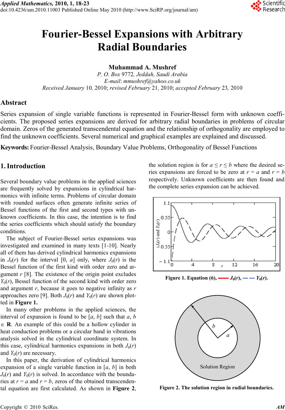Applied Mathematics, 2010, 1, 18-23
doi:10.4236/am.2010.11003 Published Online May 2010 (http://www.SciRP.org/journal/am)
Fourier-Bessel Expansions with Arbitrary
Radial Boundaries
Muhammad A. Mush ref
P. O. Box 9772, Jeddah, Saudi Arabia
Received January 10, 2010; revised February 21, 2010; accepted February 23, 20 10
Abstract
Series expansion of single variable functions is represented in Fourier-Bessel form with unknown coeffi-
cients. The proposed series expansions are derived for arbitrary radial boundaries in problems of circular
domain. Zeros of the generated transcendental equation and the relationship of orthogonality are employed to
find the unknown coefficients. Several numerical and graphical examples are explained and discussed.
Keywords: Fourier-Bessel Analysis, Boundary Value Problems, Orthogonality of Bessel Functions
1. Introduction
Several boundary value problems in the applied sciences
are frequently solved by expansions in cylindrical har-
monics with infinite terms. Problems of circular domain
with rounded surfaces often generate infinite series of
Bessel functions of the first and second types with un-
known coefficients. In this case, the intention is to find
the series coefficients which should satisfy the boundary
conditions.
The subject of Fouri er -B esse l series expansions was
investigated and examined in many texts [1-10]. Nearly
all of them has derived cylindrical harmonics expansions
in J0(r) for the interval [0, a] only, where J0(r) is the
Bessel function of the first kind with order zero and ar-
gument r [8]. The existence of the origin point excludes
Y0(r), Bessel function of the second kind with order zero
and argument r, because it goes to negative infinity as r
approaches zero [9]. Both J0(r) and Y0(r) are shown plot-
ted in Figure 1.
In many other problems in the applied sciences, the
interval of expansion is found to be [a, b] such that a, b
∈ R. An example of this could be a hollow cylinder in
heat conduction problems or a circular band in vibrations
analysis solved in the cylindrical coordinate system. In
this case, cylindrical harmonics expansions in both J0(r)
and Y0(r) are necessary.
In this paper, the derivation of cylindrical harmonics
expansion of a single variable function in [a, b] in both
J0(r) and Y0(r) is solved. In accordance with the bounda-
ries at r = a and r = b, zeros of the obtained transce nd e n-
tal equation are first calculated. As shown in Figure 2,
the solution region is for a ≤ r ≤ b where the desired se-
ries expansions are forced to be zero at r = a and r = b
respectively. Unknown coefficients are then found and
the complete series expansion can be achieved.
Figure 1. Equation (6), ▬▬ J0(r), ▬ ▬ Y0(r).
Figure 2. The solution region in radial boundaries.
Solution Region
b
a
r
J0(r) and Y0(r)

M. A. MUSHREF 19
Copyright © 2010 SciR es. AM
2. Formulation and Solution
The Bessel differential equation of order zero is well
known as [1, 4]:
0)()()(
2
2
2
=++ rrfrf
dr
d
rf
dr
d
r
α
(1)
∀
α and r ∈ R and a ≤ r ≤ b.
The general solution to Equation (1) for real values of
 is known to be [2, 3]:
∑
∞
=
+=
0
00
)()()(
n
nn
rYBrJArf αα
(2)
As in Equation (1), the assumed boundary conditions
at r = a and r = b are of Dirichlet type as f(a) = 0 and f(b)
= 0 respectively. Both An and Bn are then related as:
nn
B
aJ
aY
A)(
)(
0
0
α
α
−=
(3)
nn
B
bJ
bY
A)(
)(
0
0
α
α
−=
(4)
Going after the elimination method, the transcendental
equation can be obtained as:
0)()()()(
0000
=− aYbJbYaJ αααα
(5)
In order for Equation (5) to be satisfied, there exist
many zeros or values of  to be calculated. Thus, in all
former and coming equations  can be replaced by n
which are the zeros obtained from the transcendental
equation ∀ n ∈ I. That is:
0)()()()(
0000
=− aYbJbYaJ
nnnn
αααα
(6)
The orthogonality feature of Bessel functions can be
applied to Equation (2) by multiplying both sides by
[ ]
)()(
00
rYBrJAr
mmmm
αα +
and integrating it over all
possible values of r from a to b as:
∫
∑∫
=
∞
=
b
a
m
n
b
a
mn
drrfrrCdrrCrrC )()()()(
0
(7)
where,
)()()( 00 rYBrJArC mmmmm
αα +=
(8)
)()()(
00
rYBrJArC
nnnnn
αα +=
(9)
The terms under the summation in the left side of Eq-
uation (7) are zeros for all values of m ≠ n [5, 6, 7].
Hence, Equation (7) can be simplified to:
{ }
∫
=−
b
a
nn
drrfrCrrC0)()()(
(10)
Either Equation (3) or (4) can help. Using Equation (3)
we can obtain the Bn coefficients as:
[ ]
∫
∫
=
b
a
n
b
a
n
n
drrSr
drr frrS
B
2
0
0
)(
)()(
α
α
(11)
where, S0(nr) is given by:
)(
)(
)(
)()(
0
0
0
00
rJ
aJ
aY
rYrS
n
n
n
nn
α
α
α
αα −=
(12)
By Equation (3) or (4), the An coefficients can also be
found. Once the coefficients An and Bn are calculated, the
function f(r) can be expanded as in Equation (2).
3. Numerical Examples
The transcendental expression in Equation (6) shows a
gradual decay as  increases which mean small magni-
tudes between high zeros. This leads to the convergence
of the series in Equation (2) above as n increases. As a
consequence, a finite number of terms in Equation (2)
can be sufficient for numerical approximations.
The zeros are first evaluated using the transcendental
cross product Bessel functions equation for the interval
[a, b]. A graph of Equation (6) is shown in Figure 3 for
the solution regions [0.65, 2.5] and [0.65, 5]. Table 1
shows the first 50 zeros of Equation (6) for a = 0.65 and
b = 2.5. Zeros obtained from the transcendental equation
changes according to the values of a and b assumed for
the solution region. The data presented in Table 1 indi-
cates that the calculated zeros are not periodic and should
be calculated using a proper numerical technique.
Let’s assume that the function f(r) to be expanded as
in Equation (2) is sin(r) with a radial solution region in
[0.65, 2.5]. The coefficients Bn can be evaluated from
Equation (11) and the An coefficients are then obtained
by Equation (3). Both coefficients are shown in Tables 2
and 3 respectively for n = 0 to 49.
Figure 3. Equation (6), ▬▬ [0.65, 2.5], ▬ ▬ [0.65, 5].
J0(
α
na)Y0(
α
nb) – J0(
α
nb)Y0(
α
na)
α

20 M. A. MUSHREF
Copyright © 2010 SciR es. AM
Many variations can be noticed for the numerical val-
ues of An and Bn with a general absolute scale of < 1 ex-
cept for B0 = 2.328. Some coefficients are in the order of
×10-3 meaning that their associated terms are very small
such as B4 and A31 in Tables 2 and 3 respectively.
The function sin(r) and its approximate expansions are
plotted in Figure 4. Summation over the first 10 terms
produced an acceptable estimation in the interval [0.65,
2.5] with some apparent oscillations around the exact
function. An improved approximate expansion is also
plotted for n = 0 to 49 with less fluctuations in the same
radial domain.
Table 1. First fifty zeros of Equation (6) in [0.65, 2.5].
n
α
n
n
α
n
n
α
n
n
α
n
n
α
n
0
1
2
3
4
5
6
7
8
9
1.663
3.376
5.08
6.782
8.4815
10.182
11.881
13.579
15.279
16.977
10
11
12
13
14
15
16
17
18
19
18.676
20.374
22.073
23.771
25.47
27.168
28.866
30.564
32.263
33.961
20
21
22
23
24
25
26
27
28
29
35.659
37.358
39.056
40.754
42.452
44.151
45.849
47.547
49.245
50.943
30
31
32
33
34
35
36
37
38
39
52.642
54.34
56.038
57.736
59.434
61.133
62.831
64.529
66.227
67.925
40
41
42
43
44
45
46
47
48
49
69.624
71.322
73.02
74.718
76.416
78.115
79.813
81.511
83.209
84.907
Table 2. First fifty Bn for f(r) = sin(r) in [0.65, 2.5].
n
B
n
n
B
n
n
B
n
n
B
n
n
B
n
0
1
2
3
4
5
6
7
8
9
2.328
–0.101
–0.703
0.234
–4.8E-3
–0.181
0.455
0.030
–0.478
0.105
10
11
12
13
14
15
16
17
18
19
0.154
–0.138
0.228
0.064
–0.385
0.048
0.231
–0.110
0.082
0.081
20
21
22
23
24
25
26
27
28
29
–0.300
7.1E-3
0.267
–0.082
–0.030
0.087
–0.212
–0.024
0.272
–0.054
30
31
32
33
34
35
36
37
38
39
–0.114
0.084
–0.123
–0.047
0.250
–0.025
–0.173
0.074
–0.036
–0.061
40
41
42
43
44
45
46
47
48
49
0.206
1.3E-3
–0.205
0.057
0.042
–0.068
0.148
0.024
–0.212
0.037
Table 3. First fifty An for f(r) = sin(r) in [0.65, 2.5].
n
A
n
n
A
n
n
A
n
n
A
n
n
A
n
0
1
2
3
4
5
6
7
8
9
–0.475
0.462
–0.547
–0.114
0.675
–0.092
–0.338
0.170
–0.143
–0.111
10
11
12
13
14
15
16
17
18
19
0.424
–0.016
–0.346
0.111
0.021
–0.110
0.279
0.025
–0.333
0.070
20
21
22
23
24
25
26
27
28
29
0.126
–0.102
0.159
0.052
–0.297
0.034
0.193
–0.087
0.054
0.069
30
31
32
33
34
35
36
37
38
39
–0.242
2.1E-3
0.229
–0.067
–0.036
0.075
–0.174
–0.024
0.236
–0.044
40
41
42
43
44
45
46
47
48
49
–0.109
0.074
–0.099
–0.044
0.218
–0.019
–0.160
0.064
–0.023
–0.057
Table 4. First fifty Bn for f(r) = cos(r) in [0.65, 2.5].
n
Bn
n
Bn
n
Bn
n
Bn
n
Bn
0
1
2
3
4
5
6
7
8
9
–0.129
0.338
0.286
–0.919
2.0E-3
0.732
–0.196
–0.122
0.207
–0.433
10
11
12
13
14
15
16
17
18
19
–0.067
0.571
–0.099
–0.264
0.167
–0.199
–0.100
0.457
–0.036
–0.338
20
21
22
23
24
25
26
27
28
29
0.131
–0.030
–0.116
0.342
0.013
–0.364
0.092
0.100
–0.118
0.223
30
31
32
33
34
35
36
37
38
39
0.050
–0.351
0.053
0.195
–0.109
0.105
0.075
–0.306
0.016
0.256
40
41
42
43
44
45
46
47
48
49
–0.090
–5.5E-3
0.089
–0.237
–0.018
0.281
–0.064
–0.100
0.092
–0.153
In addition, f(r) = cos(r) is expanded as in Equation (2)
and the first fifty coefficients are listed in Tables 4 and 5
for the Bn and An respectively. Similar to the sin(r), the
cos(r) coefficients go through several variations with a
general absolute scale of < 1 except A1 = −1.550. Also,
only four coefficients are in the order of ×10-3 implying
that their related terms in the series are extremely small
such as B4 and A41 in Tables 4 and 5 respectively.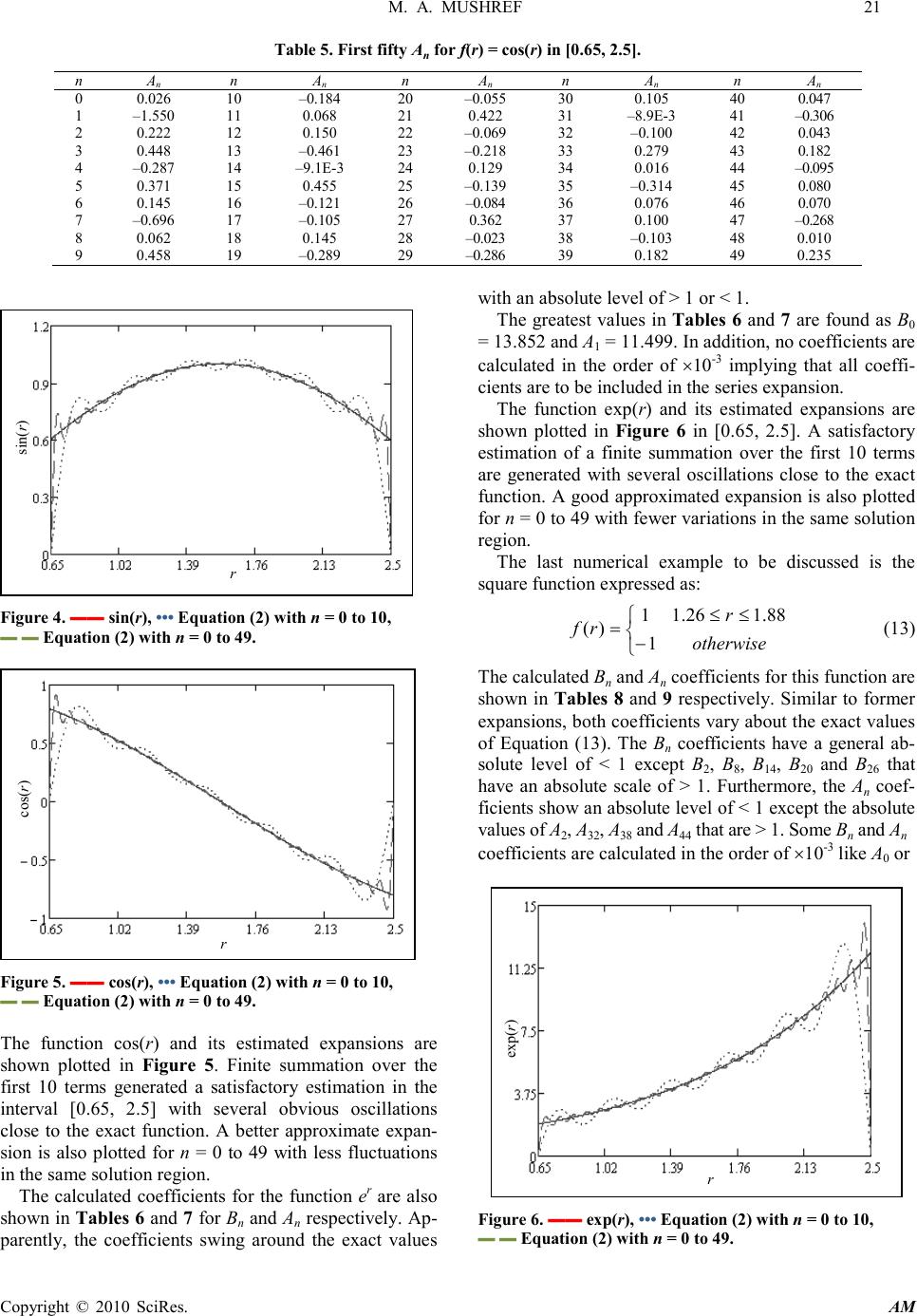

M. A. MUSHREF 21
Table 5. First fifty An for f(r) = cos(r) in [0.65, 2.5].
n
A
n
n
A
n
n
A
n
n
A
n
n
A
n
0
1
2
3
4
5
6
7
8
9
0.026
–1.550
0.222
0.448
–0.287
0.371
0.145
–0.696
0.062
0.458
10
11
12
13
14
15
16
17
18
19
–0.184
0.068
0.150
–0.461
–9.1E-3
0.455
–0.121
–0.105
0.145
–0.289
20
21
22
23
24
25
26
27
28
29
–0.055
0.422
–0.069
–0.218
0.129
–0.139
–0.084
0.362
–0.023
–0.286
30
31
32
33
34
35
36
37
38
39
0.105
–8.9E-3
–0.100
0.279
0.016
–0.314
0.076
0.100
–0.103
0.182
40
41
42
43
44
45
46
47
48
49
0.047
–0.306
0.043
0.182
–0.095
0.080
0.070
–0.268
0.010
0.235
Figure 4. ▬▬ s i n(r), ••• Equation (2) with n = 0 to 10,
▬ ▬ Equation (2) with n = 0 to 49.
Figure 5. ▬▬ cos(r), ••• Equation (2) with n = 0 to 10,
▬ ▬ Equation (2) with n = 0 to 49.
The function cos(r) and its estimated expansions are
shown plotted in Figure 5. Finite summation over the
first 10 terms generated a satisfactory estimation in the
interval [0.65, 2.5] with several obvious oscillations
close to the exact function. A better approximate expan-
sion is also plotted for n = 0 to 49 with less fluctuations
in the same solution region.
The calculated coefficients for the function er are also
shown in Tables 6 and 7 for Bn and An respectively. Ap-
parently, the coefficients swing around the exact values
with an absolute level of > 1 or < 1.
The greatest values in Tables 6 and 7 are found as B0
= 13.852 and A1 = 11.499. In addition, no coefficients are
calculated in the order of ×10-3 implying that all coeffi-
cients are to be included in the series expansion.
The function exp(r) and its estimated expansions are
shown plotted in Figure 6 in [0.65, 2.5]. A satisfactory
estimation of a finite summation over the first 10 terms
are generated with several oscillations close to the exact
function. A good approximated expansion is also plotted
for n = 0 to 49 with fewer variations in the same solution
regio n.
The last numerical example to be discussed is the
square function expressed as:



−
≤≤
=otherwise
r
rf 1
88.126.11
)(
(13)
The calculated Bn and An coefficients for this function are
shown in Tables 8 and 9 respectively. Similar to former
expansions, both coefficients vary about the exact values
of Equation (13). The Bn coefficients have a general ab-
solute level of < 1 except B2, B8, B14, B20 and B26 that
have an absolute scale of > 1. Furthermore, the An coef-
ficients show an absolute level of < 1 except the absolute
values of A2, A32, A38 and A44 that are > 1. Some Bn and An
coefficients are calculated in the order of ×10-3 like A0 or
Figure 6. ▬▬ exp(r), ••• Equation (2) with n = 0 to 10,
▬ ▬ Equation (2) with n = 0 to 49.
cos(r)
r
sin(r)
r
exp(r)
r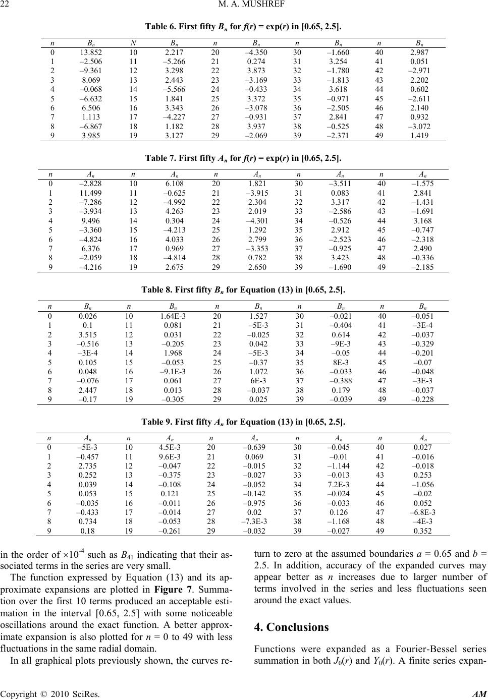

22 M. A. MUSHREF
Table 6. First fifty Bn for f(r) = exp( r) in [0.65, 2.5].
n
B
n
N
B
n
n
B
n
n
B
n
n
B
n
0
1
2
3
4
5
6
7
8
9
13.852
–2.506
–9.361
8.069
–0.068
–6.632
6.506
1.113
–6.867
3.985
10
11
12
13
14
15
16
17
18
19
2.217
–5.266
3.298
2.443
–5.566
1.841
3.343
–4.227
1.182
3.127
20
21
22
23
24
25
26
27
28
29
–4.350
0.274
3.873
–3.169
–0.433
3.372
–3.078
–0.931
3.937
–2.069
30
31
32
33
34
35
36
37
38
39
–1.660
3.254
–1.780
–1.813
3.618
–0.971
–2.505
2.841
–0.525
–2.371
40
41
42
43
44
45
46
47
48
49
2.987
0.051
–2.971
2.202
0.602
–2.611
2.140
0.932
–3.072
1.419
Table 7. First fifty An for f(r) = exp( r) in [0.65, 2.5].
n
A
n
n
A
n
n
A
n
n
A
n
n
A
n
0
1
2
3
4
5
6
7
8
9
–2.828
11.499
–7.286
–3.934
9.496
–3.360
–4.824
6.376
–2.059
–4.216
10
11
12
13
14
15
16
17
18
19
6.108
–0.625
–4.992
4.263
0.304
–4.213
4.033
0.969
–4.814
2.675
20
21
22
23
24
25
26
27
28
29
1.821
–3.915
2.304
2.019
–4.301
1.292
2.799
–3.353
0.782
2.650
30
31
32
33
34
35
36
37
38
39
–3.511
0.083
3.317
–2.586
–0.526
2.912
–2.523
–0.925
3.423
–1.690
40
41
42
43
44
45
46
47
48
49
–1.575
2.841
–1.431
–1.691
3.168
–0.747
–2.318
2.490
–0.336
–2.185
Table 8. First fifty Bn for Equation (13) in [0.65, 2.5].
n Bn n Bn n Bn n Bn n Bn
0
1
2
3
4
5
6
7
8
9
0.026
0.1
3.515
–0.516
–3E-4
0.105
0.048
–0.076
2.447
–0.17
10
11
12
13
14
15
16
17
18
19
1.64E-3
0.081
0.031
–0.205
1.968
–0.053
–9.1E-3
0.061
0.013
–0.305
20
21
22
23
24
25
26
27
28
29
1.527
–5E-3
–0.025
0.042
–5E-3
–0.37
1.072
6E-3
–0.037
0.025
30
31
32
33
34
35
36
37
38
39
–0.021
–0.404
0.614
–9E-3
–0.05
8E-3
–0.033
–0.388
0.179
–0.039
40
41
42
43
44
45
46
47
48
49
–0.051
–3E-4
–0.037
–0.329
–0.201
–0.07
–0.048
–3E-3
–0.037
–0.228
Table 9. First fifty An for Equation (13) in [0.65, 2.5].
n
An
n
An
n
An
n
An
n
An
0
1
2
3
4
5
6
7
8
9
–5E-3
–0.457
2.735
0.252
0.039
0.053
–0.035
–0.433
0.734
0.18
10
11
12
13
14
15
16
17
18
19
4.5E-3
9.6E-3
–0.047
–0.375
–0.108
0.121
–0.011
–0.014
–0.053
–0.261
20
21
22
23
24
25
26
27
28
29
–0.639
0.069
–0.015
–0.027
–0.052
–0.142
–0.975
0.02
–7.3E-3
–0.032
30
31
32
33
34
35
36
37
38
39
–0.045
–0.01
–1.144
–0.013
7.2E-3
–0.024
–0.033
0.126
–1.168
–0.027
40
41
42
43
44
45
46
47
48
49
0.027
–0.016
–0.018
0.253
–1.056
–0.02
0.052
–6.8E-3
–4E-3
0.352
in the order of ×10-4 such as B41 indicating that their as-
sociated terms in the series are very small.
The function expressed by Equation (13) and its ap-
proximate expansions are plotted in Figure 7. Summa-
tion over the first 10 terms produced an acceptable esti-
mation in the interval [0.65, 2.5] with some noticeable
oscillations around the exact function. A better approx-
imate expansion is also plotted for n = 0 to 49 with less
fluctuations in the same radial domain.
In all graphical plots previously shown, the curves re-
turn to zero at the assumed boundaries a = 0.65 and b =
2.5. In addition, accuracy of the expanded curves may
appear better as n increases due to larger number of
terms involved in the series and less fluctuations seen
around the exact values.
4. Conclusions
Functions were expanded as a Fourie r-Bessel ser ie s
summation in both J0(r) and Y0(r). A finite series expan-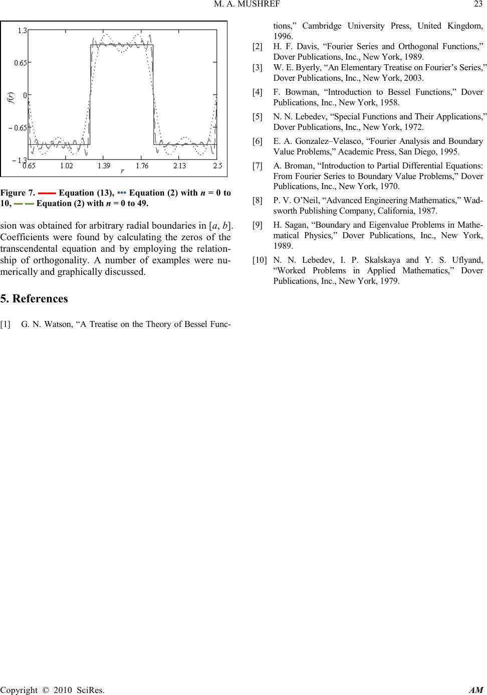

M. A. MUSHREF 23
Copyright © 2010 SciR es. AM
Figure 7. ▬▬ Equation (13), ••• Equation (2) with n = 0 to
10, ▬ ▬ Equation (2) with n = 0 to 49.
sion was obtained for arbitrary radial boundaries in [a, b].
Coefficients were found by calculating the zeros of the
transcendental equation and by employing the relation-
ship of orthogonality. A number of examples were nu-
merically and graphically discussed.
5. References
[1] G. N. Watson, “A Treatise on the Theory of Bessel Func-
tions,” Cambridge University Press, United Kingdom,
1996.
[2] H. F. Davis, “Fourier Series and Orthogonal Functions,”
Dover Publications, Inc., New York, 1989.
[3] W. E. Byerly, “An Elementary Treatise on Fourier’s Series,”
Dover Publications, Inc., New York, 2003.
[4] F. Bowman, “Introduction to Bessel Functions,” Dover
Publications, Inc., New York, 1958.
[5] N. N. Lebedev, “Special Functions and Their Applications,”
Dover Publications, Inc., New York, 1972.
[6] E. A. Gonzalez–Velasco, “Fourier Analysis and Boundary
Value Problems,” Academic Press, San Diego, 1995.
[7] A. Broman, “Introduction to Partial Differential Equations:
From Fourier Series to Boundary Value Problems,” Dover
Publications, Inc., New York, 1970.
[8] P. V. O’Neil, “Advanced Engineering Mathematics,” Wad-
sworth Publishing Company, California, 1987.
[9] H. Sagan, “Boundary and Eigenvalue Problems in Mathe-
matical Physics,” Dover Publications, Inc., New York,
1989.
[10] N. N. Lebedev, I. P. Skalskaya and Y. S. Uflyand,
“Worked Problems in Applied Mathematics,” Dover
Publications, Inc., New York, 1979.
r
f(r)