Journal of Modern Physics
Vol.4 No.1(2013), Article ID:27253,10 pages DOI:10.4236/jmp.2013.41019
Testing Some f(R,T) Gravity Models from Energy Conditions
1Department of Natural Science, Federal University of Espirito Santo, Sao Mateus, Brazil
2Institute of Mathematics and Physical Sciences (IMSP), Porto-Novo, Benin
Email: sthoundjo@yahoo.fr
Received August 17, 2012; revised October 28, 2012; accepted November 18, 2012
Keywords: Modified Gravity; Energy Conditions; Cosmological Stability
ABSTRACT
We consider  theory of gravity, where
  is the curvature scalar and T is the trace of the energy momentum tensor. Attention is attached to the special case,
  and two expressions are assumed for the function
 ,
,  and
and , where
 ,
,  ,
,  ,
,  ,
,  ,
,  ,
,  ,
,  and
and  are input parameters. We observe that by adjusting suitably these input parameters, energy conditions can be satisfied. Moreover, an analysis of the perturbations and stabilities of de Sitter solutions and power-law solutions is performed with the use of the two models. The results show that for some values of the input parameters, for which energy conditions are satisfied, de Sitter solutions and power-law solutions may be stables.
1. Introduction
It is well known that General Relativity (GR) based on the Einstein-Hilbert action (without taking into account the dark energy) can not explain the acceleration of the early and late universe. Therefore, GR does not describe precisely gravity and it is quite reasonable to modify it in order to get theories that admit ination and imitate the dark energy. The first tentative in this way is substituting Einstein-Hilbert term by an arbitrary function of the curvature scalar R, this is the so-called  theory of gravity. This theory has been widely studied and interesting results have been found [1,2]. In the same way, other alternative theory of modified gravity has been introduced, the so-called Gauss-Bonnet gravity,
  , as a general function of the Gauss-Bonnet invariant term
  [3]. Other combinations of scalars are also used as the generalised
  and
and  [4,5], where
  and
and  (here
(here  and
and  are the Ricci tensor the Riemann tensor, respectively).
In this present paper, attention is attached to a type of the so-called  theory of gravity, where
  denotes the trace of the energy momentum tensor. This generalization of
  gravity has been made first by Harko et al. [6]. In [7], the cosmological reconstruction of describing transition from matter dominated phase to the late accelerated epoch of the universe is performed. Also in the same way for exploring cosmological scenarios based on this theory,
  function has been numerically reproduced according to holographic dark energy [8]. Moreover it is shown that dust reproduces
 , phantom-non-phantom and the phantom cosmology with
  theory [9]. The general technique for performing this reproduction of
  model in FRW’s metric cosmological evolution is widely developed in [4,10]. The
  models that are able to reproduce the fourth known types of future finite-time singularities have been investigated [11].
Note that singularities appear when energy conditions are violated. Our task in this paper is to check the viability of some models of  according to the energy conditions. The energy conditions are formulated by the use of the Raychaudhuri equation for expansion and is based on the attractive character of the gravity. We refer the readers to Refs. [12-17], where energy conditions are widely analyzed for the cosmology settings, in
  and
and  gravities.
In this paper, we assume a special form of , that is,
  , the usual Einstein-Hilbert term plus a
  dependent function
 . Two expressions of
 ,
,  and
and  are investigated.
In order to reach the acceptable cosmological models, we analyse the perturbations and stabilities of de Sitter solutions and power-laws solutions in the framework of the special  gravity, by using the two models proposed in this work. We observe that for some values of the input parameters, for both models, the stabilities of de Sitter solutions and power-law solutions are realized and compatibles with some energy conditions and the late time acceleration of the universe.
The paper is outlined as follows. In Section 2, we briefly present the general formalism of the theory, putting out the general equations of motion for a  gravity, where
  and
and  and are respectively function of the curvature scalar and the trace of the energy momentum tensor. The Section 3 is devoted to the general aspects of the energy conditions. The
  gravity is assumed in the Section 4, where the two functions considered for
  are studied, putting out the conditions on the input parameters for obtaining some viable models of
 . The perturbations and stabilities of de Sitter and power-law solutions are investigated in the Sections 5. Discussions and perspectives are presented in the Section 6.
2. General Formalism
Let us assume the modified gravity replacing the Ricci scalar  in Einstein gravity by an arbitrary function
 , and writing the total action as
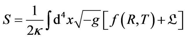 , (1)
, (1)
where ,
,  being the gravitational constant and
 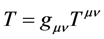 the trace of the matter energy momentum tensor which is defined by
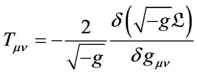 (2)
(2)
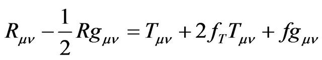
This modified gravity theory has been considered first in [6] and the equations of motion, using the metric formalism, have been explicitly obtained as
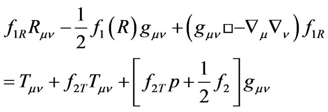 (3)
(3)
3. Energy Conditions
The energy conditions are essentially based on the Raychaudhuri equation that describes the behaviour of a congruence of timelike, spacelike or lightlike curves. For the purposes of this work we will just consider the timelike and space-like curves for which the Raychaudhuri equation reads, respectively [18,19]
 (4)
(4)
 (5)
(5)
where  is the expansion scalar describing the expansion of volume,
  and
and  are positive parameters used to describe the curved of the congruence,
  the shear tensor which measures the distortion of the volume,
  the vorticity tensor which measures the rotation of the curves, and
  and
and  are respectively timelike and lightlike vectors tangent to the curves. In this work, we are interested to the situation for small distortions of the volume, without rotation, in such a way that the quadratic terms in the Raychaudhuri equation may be disregarded (they are like second order corrections). Then, the equation can be integrated given the scalar of expansion as a function of the Ricci tensor:
 (6)
(6)
The condition for attractive gravity is , imposing
  and
and . These two conditions are called the strong and null energy conditions, respectively.
For equivalence to GR, by just dividing by  (different from zero), one can cast Equation (3) in the following form
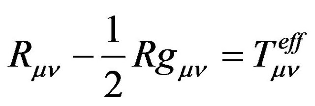 (7)
(7)
where the effective energy momentum tensor  is defined by
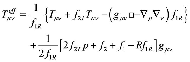 (8)
(8)
Thus, the null energy condition for the effective perfect fluid reduces to
 . (9)
. (9)
For the strong energy conditions, one has

 . (10)
The weak energy condition for the effective perfect fluid reads
 ,
,  , (11)
and the the dominant energy condition results in
 ,
,  ,
, . (12)
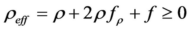
Therefore, the energy conditions, as known in GR, can also be applied in this modified theory of gravity by substituting the ordinary energy density ρ and pressure p in GR by the effective ones,  and
and .
.
In what follows, we will consider models of type , i.e., the usual Einstein-Hilbert term plus trace depending term
 . This amounts to consider
  and
and . The factor 2 is used just for letting the field equations more easier to be treated. We will also assume that the ordinary content of the universe is pressureless and satisfies the energy conditions (just
 ).
).
4. Testing Some  Models from Energy Conditions
In this section we will present the conditions required on  and the algebraic function
  for realizing each type of energy conditions. For this end, we first need to establish the respective expression of the effective energy density
  and effective pressure
 . According to the assumptions made at the end of the previous section, Equation (7) becomes
 . (13)
Considering the at FRW space-time described by the metric
 (14)
(14)
where a(t) is the scale factor. The 00 and ii components of (22) can be written as
 , (15)
 , (16)
where the effective energy density and pressure are defined as
 , (17)
 . (18)
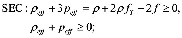
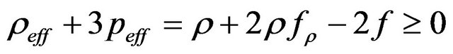
By using the above expressions of the effective energy density and pressure, we get the null energy condition (NEC), the weak energy condition (WEC), the strong energy condition (SEC) and the dominant energy condition (DEC) by NEC: ; (19)
WEC: ,
, ; (20)
 (21)
(21)
 (22)
(22)
and  is assumed to be positive and non-null. This form is chosen due to its interesting aspect, in curing the big rip [11].
4.1. Studing the Case 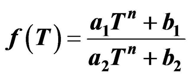
Our task here is to put out the constraints on the input parameters in order to get a  type model that satisfies the energy conditions. According to the sign of the parameter
 , and assuming that
  and
and  cannot be identically null, the model can be cast into two different forms. In fact, for the late time stage of the universe, by dividing the parameters of the model by
  and
and , one gets respectively the models
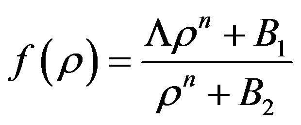 and
and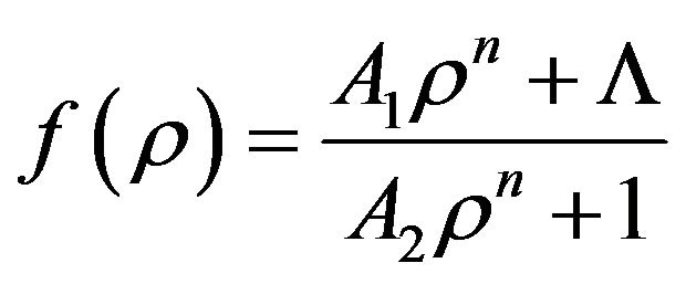 , where the cosmological constant is characterized by
  (for
(for ), and
  (for
(for ), and
 ,
, ,
,  and
and . In this case, the model which initially was four parameters dependent, under the cosmological constraints, becomes three parameters dependent,
  ,
, and
and  for
for , and
, and ,
,  and
and  for
for . Since the cosmological constant is known [14], the model turns into two parameters dependent.
The first derivative of  with respect to
  (or the derivative of
  with respect to
 ) reads
 (23)
(23)
4.1.1. The NEC
Since we have assumed that the ordinary content of the universe satisfies all the energy conditions, the condition (19) reduces to , (or
, (or ). One can calculate
  as
as
 (24)
(24)
 (25)
(25)
whose the sign can just be characterized by that of the numerator, since the denominator is always positive. If we take the numerator as a function of the ordinary energy density  and the input parameters, we just need to analyze the sign of this latter. The evident conditions for which the numerator is positive are presented as follows:
* ,
,  ,
,  for
for *
* ,
,  ,
,  for
for *
* ,
,  , for
, for *
* ,
,  , for
, for .
.
Indeed, the above conditions lead to the positivity
 for
for 
and
 for
for .
.
Observe that there are still situations in which the above quantities are negative but the numerators in (25) continuing positive, i.e.*  and
and 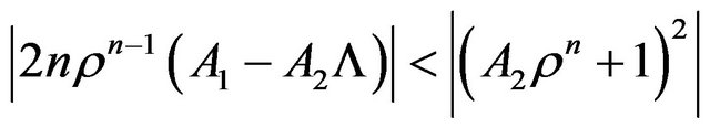 for
for *
*  and
and 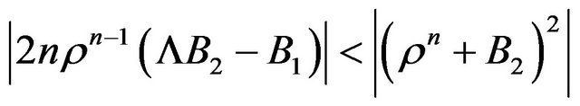 for
for .
.
In these cases, one can plot the function in terms of two of the parameters, fixing the other. Despite knowing the sign of the considered parameters with what respect the function may be plotted, the important here is their rank, i.e. the interval to which they must belong in order to produce the positivity of the function. Some examples are presented in Figure 1.
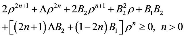
4.1.2. The WEC
This condition is realized when the NEC is, plus the condition . Note that the complete expression and condition of the NEC read
 , (26)
 . (27)
These expressions are obtained by multiplying the numerators in (25) by . We didn’t need to use this complete expression for determining the conditions on the input parameters in the case of the NEC, since the
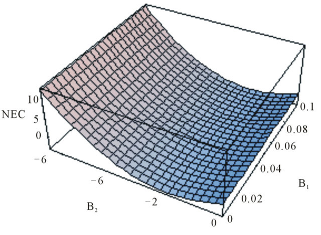
Figure 1. The graph representing the NEC in functions of  and
and  with
with ,
,  ,
, .
.
ordinary energy density is assumed as positive quantity. Besides to (26) and (27), the second condition for satisfying the WEC is
 , (28)
having in mind that the ordinary content is assumed as pressure-less. By using , according to the functions in (23), (28) becomes
 (29)
(29)
 (30)
(30)
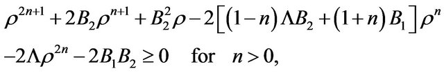
Note here that we just use the numerator of the fractions whose the denominators are always positives. By combining (26) with (29) and (30), one gets for the WEC
 (31)
(31)
 (32)
(32)
We address here the evident conditions for which the WEC is satisfied as follows:
* 
 for
for 
* 
 for
for .
.
It is obvious that these conditions are not unique. For n > 0 (n < 0), the necessity of plotting the function
 (33)
(33)
 (34)
(34)
varying two of the input parameters. We present some examples of these cases in Figure 2.
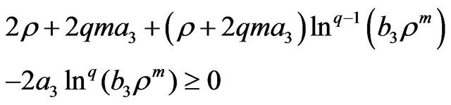
4.1.3. The SEC
The strong energy condition is realized by combining the NEC with . This latter reads,
 . (35)
Making use of the expressions in (23), one obtains a fraction whose the denominator is always positive and the numerator reads
 (36)
(36)
 (37)
(37)
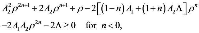
Figure 2. The graph of WEC in terms of suitable values of  and
and  with
with ,
,  ,
, .
.
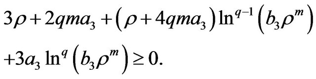
Now, combining (36) and (37) with the NEC, on gets the following conditions for the SEC
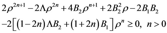 (38)
(38)
 . (39)
In this case, there is any obvious condition for satisfying the SEC. However, values can be found, by plotting the corresponding functions in terms of two of the parameters. Some examples for illustrating some of these cases are presented in Figure 3.
4.1.4. The DEC
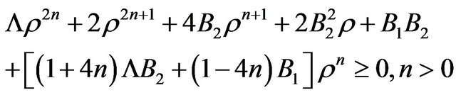
The dominant energy condition is characterized by the WEC combined with . Following the same steps as in the previous cases, one easily obtains the DEC as
 (40)
(40)
 (41)
(41)
The evident conditions read ,
,  and
and . Evidently, other conditions may lead to the accomplishment of the DEC, but, only plotting the functions in (40) and (41). We present some of these cases in Figure 4.
4.2. Studying the Case 
Here we will work with the fundamental conditions for which the model allows the avoidance of the Big Rip. So,

Figure 3. The graph of the SEC in functions of  and
and , setting
 ,
,  and
and .
.
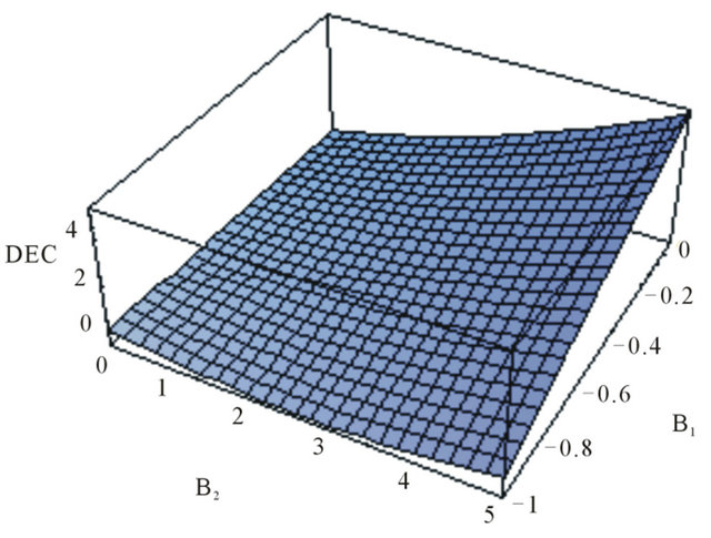
Figure 4. The graph representing the DEC in functions of  and
and  with
with ,
,  ,
, .
.
we propose to check if the range of parameters for which the singularity may be cured can also make the model satisfying the energy conditions. Here, the first derivative of  also plays an important role. Deriving
  with respect to the energy density
 , one gets
 (42)
(42)
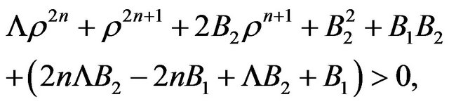
We believe that each step of constructing the four energy conditions is now clear and we simply present the results and comments as follows:
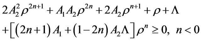
4.2.1. The NEC
 . (43)
The evident conditions for obtaining this are ,
,  ,
, , with
 . It is important to note that this list is not exhaustive, since in other conditions different from the above ones, the NEC could still be realized. This situation requires knowing some intervals to which the parameters must belong. We present this feature by plotting the function corresponding to the expression (43) in terms of some of the input parameters fixing the other. See Figure 5.
4.2.2. The WEC
 (44)
(44)
In this case by plotting the function (44), the WEC can be realized graphically. This is the set of situations where one of the terms in the sum (44) is negative, but it absolute value is less that the absolute value of the sum of the other. See Figure 6.
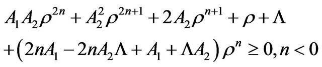
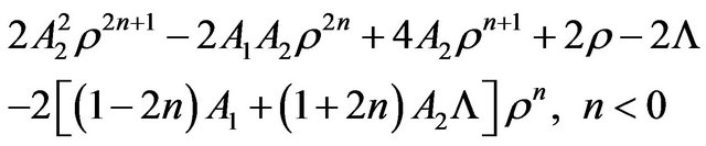
4.2.3. The SEC
 (45)
(45)
In this case, evident constraints on the input parameters in order to realize this energy conditions are presented as follows: ,
,  ,
,  , with
 . As presented in the previous cases, other conditions may also realize this energy conditions. This can be observed by plotting the function in (45) in terms of some input parameters, fixing the other. See Figure 7.
4.2.4. The DEC
 (46)
(46)
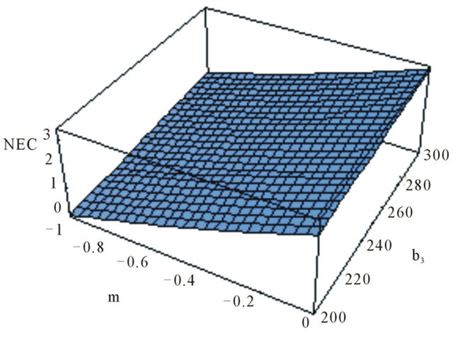
Figure 5. The graph representative of the NEC in terms of m and , with
 ,
,  and
and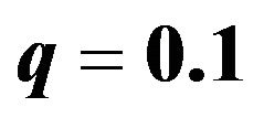 .
.
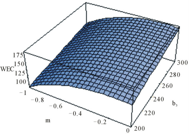
Figure 6. The graph of the WEC in functions of m and b3, using ,
,  and
and .
.
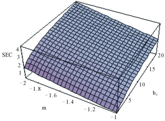
Figure 7. The graph of the SEC in functions of  and
and , using
 ,
,  and
and .
.
Here, constraints may also lead to the DEC, but this is clear by plotting the function (46), as in the previous cases. We present an illustrative example in Figure 8.
We mention that for all the graphs, the parameters are normalized to  Planck units. Remark that the current value of the cosmological constant is about
  and the energy density of the usual matter is about
  [14]. Then, with the normalization, we get
  and
and  for the cosmological constant and the energy density of the usual matter respecttively, which are the values used for plotting the graph in the figures.
5. Perturbations and Stabilities in R + 2f(T) Gravity
In this section we propose to study the perturbations around the models used in this work. We can start establishing the perturbed equations for the case ,
,
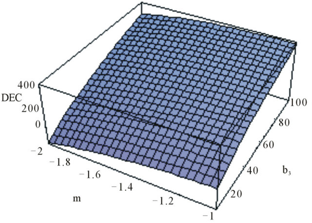
Figure 8. The graph of the WEC in functions of m and b3, with ,
,  and
and .
.
but the two models will be studied as specific cases.
For this purpose, let us assume a general solution for the cosmological background of FRW metric, which is given by a Hubble parameter  that satisfies the background Equation (17) using (15), for
  gravity. The evolution of the matter energy density can be expressed in terms of this particular solution by solving the continuity equation around
 ,
,
 , (47)
yielding
 . (48)
We recall that we are considering that the ordinary content of the universe is pressure-less. Since we are interesting in studying the perturbations around the solutions , we will consider small deviations from the Hubble parameter and the energy density, i.e., we can write the Hubble parameter and the ordinary energy density as [20]
 . (49)
In order to study the behavior of these perturbations in the linear regime, we expand the function  in powers of
  (or
(or ) evaluated at the solution
 , as
, as
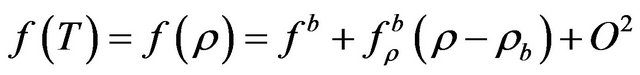 , (50)
where the superscript b refers to the background values of  and its derivatives evaluated at
  (or
(or ). Here, the O term includes all the terms proportional to the square or higher powers of
  (or
(or ). Then, only the linear terms of the induced perturbations will be considered. Hence, by making use of the expression (50) in the Equations (15) and (17), one gets the equation for the perturbation δ(t) in the linear approximation,
 (51)
(51)
On the other hand, there is a second perturbed equation from the matter continuity equation,
 . (52)
By combining Equations (51) and (52) one gets the following equation for the matter perturbation
 , (53)
from which we obtain
 , (54)
where C1 is an integration constant. By using the relation (52), the perturbation δ reads
 . (55)
Let us now consider two cosmological solutions and analyze their stability by the use of the models treated in this work: de Sitter solutions and power law solutions.
5.1. Stability of de Sitter Solutions
In de Sitter solutions, the Hubble parameter is constant and one has
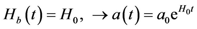 , (56)
where  is constant.
With this scale factor, the energy density of the background becomes , with which one has
 . By using this, one can cast the integral in (55) into
 . (57)
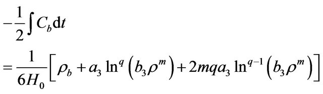
5.1.1. Treating the Model 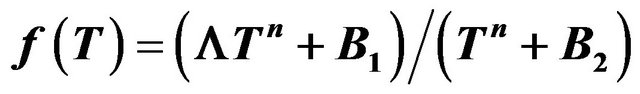
This case corresponds to n > 0, and the integral (55) can be expressed as
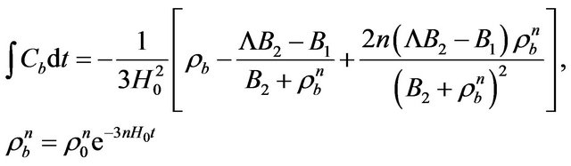 (58)
(58)
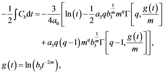
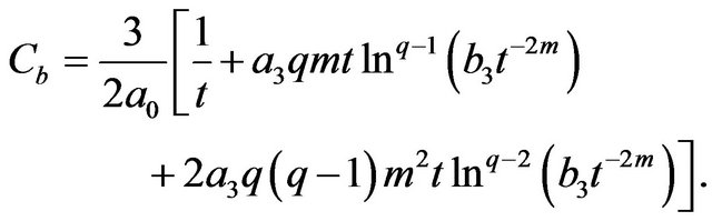
and Cb is written as
 (59)
(59)
We see from (58) and (59) that for , and as the time evolves, the stability of de Sitter solutions requires
 . In other word, for the initial model, de Sitter solutions are stables if and only if
  and
and .
.
5.1.2. Testing the Model 
This case corresponds to , and the integral (57), multiplied by
 , can be expressed as
 (60)
(60)
and Cb is written as
 (61)
(61)
Here, for , as the time evolves, both (60) and (61) tend to
 . Thus the perturbation will grow exponentially, and this particular de Sitter solution becomes unstable. Note that this result does not depend on any of the parameters
  or
or .
.
5.1.3. Treating the Model 
With this model, the integral (57), multiplied by , can be performed and one gets
 (62)
(62)
with the corresponding expression of  being
being
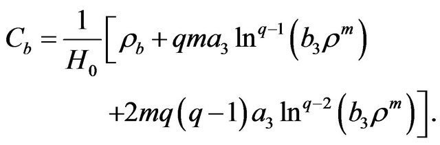 (63)
(63)
Let us recall that this model , leads to the avoidance of the Big Rip for
  and
and , where
 , as we have previously shown. These conditions also allow the model to satisfy the energy conditions. Now, let us check what happens about the stability with these conditions. First, note that the relation
  can be cast into
  , showing that
  because of
 . By choosing
 , we see that, within the conditions
  and
and , the expressions (62) and (63) tend to
  as the time evolves, and this ensures the decay of the perturbation, leading to the stability of de Sitter solutions with this model. Thus, regarding to the stability of de Sitter solutions, the energy conditions and the late time acceleration, provided with the conditions
 ,
,  ,
, and
and , we can conclude that the model may be cosmologically acceptable.
5.2. Stability of Powerlaw Solutions
As we are dealing with dust as ordinary content of the universe, we will be interested to the scale factor
 . (64)
5.2.1. Treating the Model 
In this case,  , and one can perform the integral
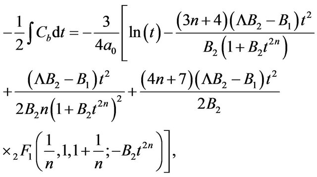 (65)
(65)
with
 , (66)
where we have set , and
, and  is the hypergeometric function defined by
 , (67)
with
 . (68)
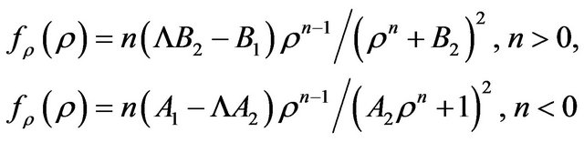
As the time evolves, conditions are required for guaranteeing the decay of the perturbation. For , it is necessary to have
 , which means that
  can be positive, or negative but with
 . In the case where
  one may observe two sub-cases, i.e., for an even
 , and an odd
 . For an even
 , as the time evolves, the necessary condition for guaranteeing the decay of the perturbation is
 , meaning that the parameter B1 can be negative, or positive. On the other hand, for an odd r, the requirement for getting the decay of the perturbation is
 , meaning that
 .
.
5.2.2. Treating the Model 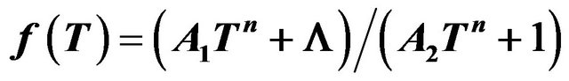
Here,  , and the integral can be performed as
 , (69)
with
 (70)
(70)
As the time evolves, the argument of the hypergeometric function tends to zero and the hypergeometric function tends to 1. Thus, the dominant term in (77) reads
 . (71)
Here, one can distinguish two cases: ( and
and ) and (
 and
and ). In the first case, one gets
  meaning that A2 can be positive, or negative but with
 . When
 ,
,  can be positive or negative, due to the relation
 , while for
 ,
,  is necessarily negative. In the second case, one gets
 , meaning that
 , which allows
  to be positive, due to the relation
 .
.
We observe that some of the conditions for which the stability occurs, are also compatible with some energy conditions. This shows that for some values of the input parameters, acceptable models can be obtained, at least regarding to the energy conditions, the stability, the late time acceleration of the universe and the avoidance of the Big Rip.
5.2.3. Treating the Model .
.
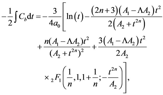
As we have done in the previous cases, the integral can be performed, yielding
 (72)
(72)
with
 (73)
(73)
As we have previously mentioned, this model cures the Big Rip for  and
and . With these conditions, as the time evolves, only the term
  grows. Since
  is negative for large value of the time, it is easy to observe that the perturbation decays, and this corresponds to the stability of the power law solutions with this model. Observe that in this case, the constraints on the parameters
  and
and  for which all the energy conditions are satisfied, leads to the stability of the power-law solutions. Thus, regarding to the stability, the energy conditions, the late time acceleration of the universe and the avoidance of the Big Rip, we can conclude that this model can be cosmologically acceptable for
 ,
,  ,
,  and
and .
.
6. Discussions
We studied the viability of two  models according to energy conditions. A special attention is attached to the models of type
 . For the two models of
  considered, it is shown that for some values of the input parameters, energy conditions are satisfied. Moreover, we showed that there exist values of the inputs parameters for which the four energy conditions may be satisfied simultaneously, for the two models.
An interesting feature of these models is that there fill well with the observations data. Therefore, the graph representing each energy conditions in plotted for both models under study.
Moreover, in order to make a consistent analysis of the stability of the models, we studied the stability of de Sitter and power-law solutions within the two models by considering the perturbation around them. We see that the de Sitter solutions present stability for two models. However, for the power-law solutions, the stability can be observed for each model under some conditions. We also see that for the conditions for which the stability is realized, the late-time cosmic acceleration and the avoidance of the big rip are always satisfied. We conclude that, in the frame work of  gravity the two models can be viable.
7. Acknowledgements
M. J. S. Houndjo thanks Prof. S. D. Odintsov for useful suggestions and also CNPq/FAPES for financial support. A. V. Monwanou thanks IMSP-UAC for financial support. The authors also thank very much the referees for useful suggestions for the reorganization of the manuscript.
REFERENCES
- S. Nojiri and S. D. Odintsov, “Introduction to Modified Gravity and Gravitational Alternative for Dark Energy,” International Journal Geometrical Method Modern Physics, Vol. 4, No. 1, 2007, p. 115. doi:10.1142/S0219887807001928
- S. Nojiri and S. D. Odintsov, arXiv: 0801.4843 [astro-ph]. arXiv: 0807.0685 [hep-th].
- S. Nojiri, S. D. Odintsov and P. V. Tretyakov, “From Inflation to Dark Energy in the Non-Minimal Modified Gravity,” Progress of Theoritical Physics Supplement, No. 172, 2008, pp. 81-89. doi:10.1143/PTPS.172.81
- A. de la Cruz-Dombriz and D. Seaz-Gomez.
- S. Nojiri and S. D. Odintsov, “Modified Gauss-Bonnet Theory as Gravitational Alternative for Dark Energy,” Physical Letter B, Vol. 613, No. 1-2, 2005, pp. 1-6. doi:10.1016/j.physletb.2005.10.010
- T. Harko, F. S. Lobo, S. Nojiri and S. D. Odintsov, “f(R,T) Gravity,” Physical Review D, Vol. 84, No. 2, 2011, Article ID: 024020. doi:10.1103/PhysRevD.84.024020
- M. J. S. Houndjo, “Reconstruction of f(R,T) Gravity Describing Matter Dominated and Accelerated Phases,” International Journal of Modern Physics D, Vol. 21, 2012, Article ID: 1250003.
- M. J. S. Houndjo and O. F. Piattella, “Reconstructing f(R, T) Gravity from Holographic Dark Energy,” International Journal of Modern Physics D, Vol. 21, No. 3, 2012, Article ID: 1250024. doi:10.1142/S0218271812500241
- M. Jamil, D. Momeni, M. Reza and R. Myrzakulov, “Reconstruction of Some Cosmological Models in f(R,T) Gravity,” European Physics Journal C, Vol. 72, 2012, p. 1999. doi:10.1140/epjc/s10052-012-1999-9
- S. Nojiri, S. D. Odintsov and D. Saez-Domez, “Cosmological Reconstruction of Realistic Modified F(R) Gravities,” Physical Letter B, Vol. 681, No. 1, 2009, pp. 74-80. doi:10.1016/j.physletb.2009.09.045
- M. J. S. Houndjo, C. E. M. Batista, J. P. Campos and O. F. Piattella, “Finite-Time Singularities in f(R,T) and the Effect of Conformal Anomaly,” arXiv: 1203.6084 [gr-qc].
- J. Santos, J. S. Alcaniz, N. Pires and M. J. Reboucas, “Energy Conditions and Cosmic Acceleration,” Physical Review D, Vol. 75, No. 8, 2007, Article ID: 083523. doi:10.1103/PhysRevD.75.083523
- S. E. Perez Bergliaffa, “Constraining f(R) Theories with the Energy Conditions,” Physical Letter B, Vol. 642, No. 4, 2006, pp. 311-314. doi:10.1016/j.physletb.2006.10.003
- J. D. Barrow and D. J. Shaw, “The Value of the Cosmological Constant,” General Relativity and Gravitation, Vol. 43, No. 10, 2011, pp. 2555-2560. doi:10.1007/s10714-011-1199-1
- J. Santos and J. S. Alcaniz, Physical Letter B, Vol. 619, 2005, p. 11; M. Visser, Science, Vol. 276, 1997, p. 88; Physical Review D, Vol. 56, 1997, p. 7578.
- D. Brown, “Action Functional for Relativistic Perfects Fluids,” Classical and Quantum Gravity, Vol. 10, No. 8, 1993, pp. 1579-1606. doi:10.1088/0264-9381/10/8/017
- N. M. García, T. Harko, F. S. N. Lobo and J. P. Mimoso, “Energy Conditions in Modified Gauss-Bonnet Gravity,” Physical Review D, Vol. 83, 2011, Article ID: 104032.
- S. W. Hawking and G. F. R. Ellis, “The Large Structure of Space-Time,” Cambridge University Press, Cambridge 1999.
- M. O. Tahim, R. R. Landim and C. A. S. Almeida, “Spacetime as a Deformable Solid,” arXiv: 0705.4120 [gr-qc].
- A. de la Cruz-Dombriz and D. Saez-Gomez.