Journal of Modern Physics
Vol.3 No.8(2012), Article ID:21669,12 pages DOI:10.4236/jmp.2012.38105
Majorana Neutrino Oscillations in Vacuum
1Escuela de Física, Universidad Pedagógica y Tecnológica de Colombia, Tunja, Colombia
2Departamento de Fsica, Universidad Nacional de Colombia, Ciudad Universitaria, Bogotá D.C., Colombia
Email: yuber.perez@uptc.edu.co, cjquimbayh@unal.edu.co
Received May 23, 2012; revised June 19, 2012; accepted July 3, 2012
Keywords: Majorana Fermions; Majorana Neutrino Oscillations; Transition Probability; Non-Relativistic and Ultra-Relativistic Approximations
ABSTRACT
In the context of a type I seesaw scenario which leads to get light left-handed and heavy right-handed Majorana neutrinos, we obtain expressions for the transition probability densities between two flavor neutrinos in the cases of lefthanded and right-handed neutrinos. We obtain these expressions in the context of an approach developed in the canonical formalism of Quantum Field Theory for neutrinos which are considered as superpositions of mass-eigenstate plane waves with specific momenta. The expressions obtained for the left-handed neutrino case after the ultra-relativistic limit is taking lead to the standard probability densities which describe light neutrino oscillations. For the right-handed neutrino case, the expressions describing heavy neutrino oscillations in the non-relativistic limit are different respect to the ones of the standard neutrino oscillations. However, the right-handed neutrino oscillations are phenomenologically restricted as is shown when the propagation of heavy neutrinos is considered as superpositions of mass-eigenstate wave packets.
1. Introduction
Neutrino physics is a very active area of research which involves some of the most intriguing problems in particle physics. The nature of neutrinos and the origin of the small mass of neutrinos are two examples of these kinds of problems. Since neutrinos are electrically neutral, the nature of these elementary particles can be Majorana or Dirac fermions. The first possibility, i.e. neutrinos being Majorana fermions was introduced by Etore Majorana [1] when he suggested that massive neutral fermions with specific momenta have associated only two helicity states implying that neutrinos and anti-neutrinos are the same particles. The second possibility implies that Dirac neutrinos are described by four-component spinorial fields which are different from spinorial fields describing antineutrinos. In this work, we will consider neutrinos as Majorana fermions which is favored by simplicity because they have only two degrees of freedom [2,3].
Direct and indirect experimental evidences show that neutrinos are massive fermions with masses smaller than 1 eV [4]. The most accepted way to generate neutrino masses is by mean of the seesaw mechanism [5]. Mass for neutrinos is a necessary ingredient to understand the oscillations between neutrino flavor states which have been observed experimentally [4]. Neutrino oscillations are originated by the interference between mass states whose mixing generates flavor states. This phenomenon means that a neutrino created in a weak interaction process with a specific flavor can be detected with a different flavor. Neutrino oscillations were first described by Pontecorvo [6] as an extension for the leptonic sector of the strange oscillations observed in the neutral Kaon system. Neutrino oscillations can be described in context of Quantum Mechanics [7-11] as an application of the two level system [12].
Description of neutrino oscillations in the context of Quantum Field Theory (QFT) is a very well studied topic [13-20]. In the literature it is possible to find two kinds of QFT models describing neutrino oscillations: intermediate models and external models [17]. In the framework of intermediate models Sassaroli developed a model based in an interacting Lagrangian density which includes the coupling between two flavor fields [21-23]. This model was framed by Beuthe as a hybrid model owing to it goes half-a-way to QFT [17]. Sassaroli model was first developed for a coupled system of two Dirac equations [21, 22] and then it was extended for a coupled system of two Majorana ones [23]. The probability amplitude of transition between two neutrino flavor states for these two systems [21-23] was obtained starting from flavor states which are used on the standard treatment of neutrino oscillations.
The standard definition of flavor states can originate some possible limitations in the description of neutrino oscillations as was observed by Giunti et al. [24]. Specifically, in reference [24] it was shown that flavor states can define an approximate Fock space of weak states in the following two cases: 1) In the extremely relativistic limit, i.e. if neutrino momentum is much larger than the maximum mass eigenvalue of a neutrino mass state; 2) for almost degenerated neutrino mass eigenvalues, i.e. if the differences between neutrino mass eigenvalues are much smaller than the neutrino momentum. The first case leads to the standard definition of flavor states. The second case has associated a real mixing matrix which is restricted to a specific interaction process. Additionally these authors have proposed that oscillations can be described appropriately for ultra-relativistic and non-relativistic neutrinos by defining appropriate flavor states which are superpositions of mass states weighted by their transitions amplitudes in the process under consideration [24].
By considering the limitations mentioned in the last paragraph it was set down by Beuthe in [17] that Sassaroli hybrid model can only be applied consistently if lepton flavor wave functions are considered as observable and the ultra-relativistic limit is taken into account. On the other hand, the Sassaroli model describing Majorana neutrino oscillations [21,22] was developed without considering the four-momentum conservation for neutrinos which implies the existence of a specific momentum for every neutrino mass state.
The main goal of this work is to study neutrino oscillations in vacuum between two flavor states considering neutrinos as Majorana fermions and to obtain the probability densities of transition for left-handed neutrinos (ultra-relativistic limit) and for right-handed neutrinos (non-relativistic limit). This work is developed in the context of a type I seesaw scenario which leads to get light left-handed and heavy right-handed Majorana neutrinos. In this context, we perform an extension of the model developed by Sassaroli in which the Majorana neutrino oscillations are obtained for the case of flavor states constructed as superpositions of mass states [21, 22]. Our extension consists in considering neutrino mass states as plane waves with specific momenta. The model that we consider in this work, which is developed in the canonical formalism of Quantum Field Theory, has the advantage that in the same theoretical treatment it is possible to study neutrino oscillations for light neutrinos and for heavy neutrinos. To do this, we first perform the canonical quantization procedure for Majorana neutrino fields of definite masses and then we write the neutrino flavor states as superpositions of mass states using quantum field operators. Next we calculate the probability amplitude of transition between two different neutrino flavor states for the light and heavy neutrino cases and we establish normalization and boundary conditions for the probability density. These probability densities for the left-handed neutrino case after the ultra-relativistic limit is taking lead to the standard probability densities which describe light neutrino oscillations. For the righthanded neutrino case, the expressions describing heavy neutrino oscillations in the non-relativistic limit are different respect to the ones of the standard neutrino oscillations. However, the right-handed neutrino oscillations are phenomenologically restricted as is shown when the propagation of heavy neutrinos is considered as superpositions of mass-eigenstate wave packets [25]. The oscillations do not take place in this case because the coherence is not preserved: in other words, the oscillation length is comparable or larger than the coherence length of the neutrino system [25].
The content of this work has been organized as follows: In Section 2, after establishing the Majorana condition, we obtain and solve the two-component Majorana equation for a free fermion; in Section 3, we consider a type I seesaw scenario which leads to get light left-handed neutrinos and heavy right-handed neutrinos; in Section 4, we obtain the Majorana neutrino fields with definite masses, then we carry out the canonical quantization procedure of these Majorana neutrino fields and we obtain relation between neutrino flavor states and neutrino mass states using operator fields; in Section 5, we determine the probability density of transition between two left-handed neutrino flavor states, additionally we establish normalization and boundary conditions and then we obtain left-handed neutrino oscillations for ultra-relativistic light neutrinos; in Section 6, we study the right-handed neutrino oscillations for non-relativistic heavy neutrinos; finally, in Section 7 we present some conclusions.
2. Two-Component Majorana Equation
In 1937 Ettore Majorana proposed a symmetric theory for electron and positron through a generalization of a variational principle for fields which obey Fermi-Dirac statistics [1]. When this theory is applied to a neutral fermion which has a specific momentum then there exist only two helicity states. The Majorana theory implies that it does not exist antiparticles associated to these fermions, i.e. Majorana fermions are their own antiparticles. For convenience we study the equation of motion for neutral fermions but using the two-component theory developed by Case in [26].
In contrast with a Dirac fermion, a Majorana fermion can only be described by a two-component spinor. To show it we consider a free relativistic fermionic field  of mass m described by the Dirac equation
 , where Dirac matrixes
  obey the anticonmutation relations
  and metric tensor satisfies
 . Using the chirality matrix given by
 , the leftand right-handed chiral projections of the fermion field ψare
 , respectively. If we write the Dirac matrixes projected on the chiral subspace as
 , we obtain that the coupled equations for the chiral components of the fermionic field
  are given by
 (1)
(1)
 (2)
(2)
We introduce the charge conjugation operation that will allow us to describe Majorana fermions. The charged conjugated field (or conjugated field)  is defined as
 (3)
(3)
where the charge conjugation operator  satisfies the properties
 ,
,  ,
,  [3]. Using these properties we find that the conjugated field
  obeys the Dirac equation
 . As
. As  describes a fermion with a specific charge, its conjugated field
  represents a fermion with an opposite charge and with the same mass, i.e.
  describes the antifermion of
 . The Dirac equation for
  should be projected on the chiral subspace and for this reason it is necessary to remember that
  [3]. So the coupled equations for the chiral components of the conjugated field
  are
are
 (4)
(4)
 (5)
(5)
We observe that the chiral components of the fermionic field  under charge conjugation
 ,
,  and the chiral components of the conjugated field
 ,
,  are related by
 ,
, 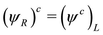 showing how the charge-conjugation operation changes the chirality of fields.
We define the Majorana condition by taking the fermionic field as proportional to the conjugated field
 (6)
(6)
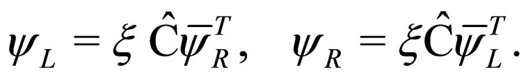
where the proportional constant is a complex phase factor of the form  which plays an important role on applications of Majorana theory. The Equality (6) implies that Majorana fermions are their own antiparticles. Now the chiral components of the Majorana field satisfy
 (7)
(7)
So we can write Equations (1) and (2) in the form
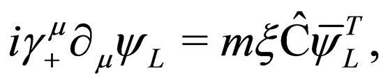 (8)
(8)
 (9)
(9)
If we apply the Majorana condition (7) into the Equations (4) and (5), we obtain Equations (8) and (9). Additionally we can observe that Equations (8) and (9) are related to themselves by means of a complex conjugation. In this way, we have gone from four coupled equations describing a fermion and its antifermion to two decoupled equations describing a left-handed chiral field  and a right-handed chiral field
 . Due to the fact that the right-handed chiral field can be constructed from the left-handed chiral field [26], as it is shown in (7), now we have only an independent field given by
 . For the last fact, we will be able to describe Majorana fermion by means of field
  which now has two components. To verify this sentence we rewrite Equation (8) as
 (10)
(10)
If we define
 (11)
(11)
and if we take , then Equation (10) can be written as
 (12)
(12)
which is known as the Majorana equation. This equation in which a particle is indistinguishable from its antiparticle has two components because the matrixes  are projected on the chiral subspaces of two components. The matrixes
  are called Majorana matrixes and these should not be confused with the Dirac matrixes written in Majorana representation.
Now we are interested in knowing the kind of relations that Majorana matrixes  obey. So we first apply definition (11) into Equation (9) and we obtain
 , with
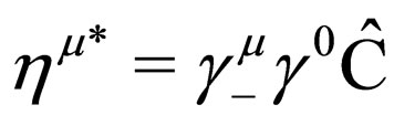 . Then we apply
  into (12) and we have
 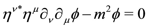 or its equivalent
 where we have used
 . Accordingly, Majorana matrixes should satisfy relations
 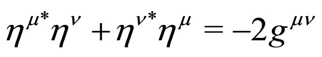 and then the field
  is satisfying the Klein-Gordon equation given by
 .
.
In this work we have taken a particular representation of matrixes  which has permitted us to write the twocomponent Majorana equation in the form given by (12). Now we can consider a matrix
  which satisfies the following relations [26]
 (13)
(13)
where  represents Pauli matrixes in a given representation. We take
 , where
  being
being  the unit matrix
  and
and  Pauli matrixes. Since
  satisfies properties (13), we have taken
  So the Equation (12) can be written as
 (14)
(14)
This equation is the well known two-component Majorana equation [27,28], which will be solved in next subsection.
Canonical Quantization for Majorana Field
With the purpose of studying the canonical quantization for the Majorana field we will obtain the free-particle solution of Equation (14). On the outset, we consider bispinors  which obey the following relations
 (15)
(15)
 (16)
(16)
where these bi-spinors correspond to helicity eigenstates. If we take the momentum in spherical coordinates , then the helicity operator has the form
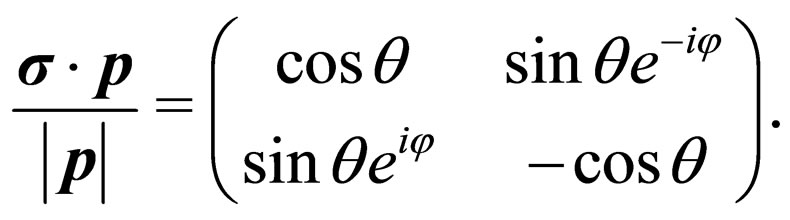 (17)
(17)
We choose the following representation for these bispinors
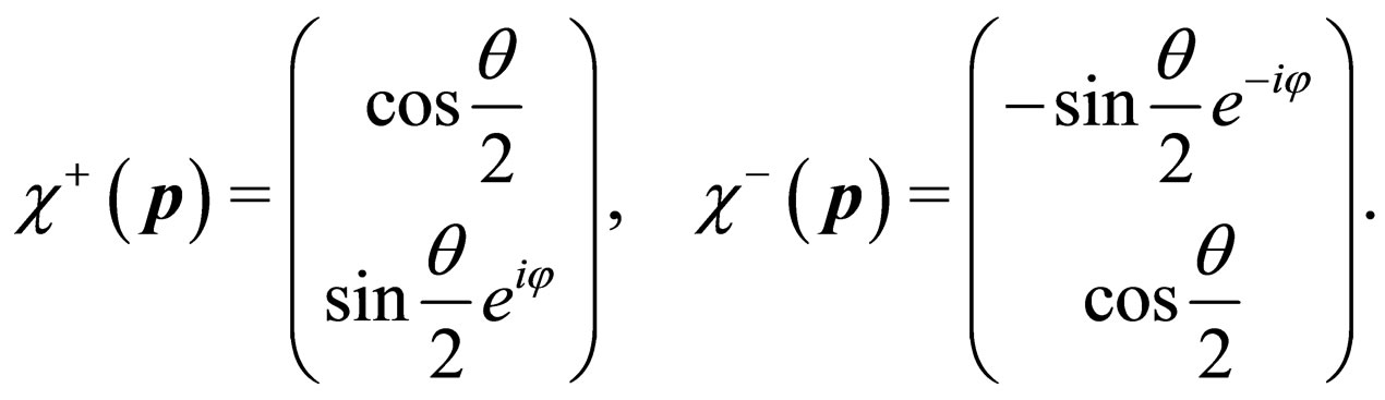 (18)
(18)
We can prove that the following solution satisfies the two-component Majorana Equation (14)
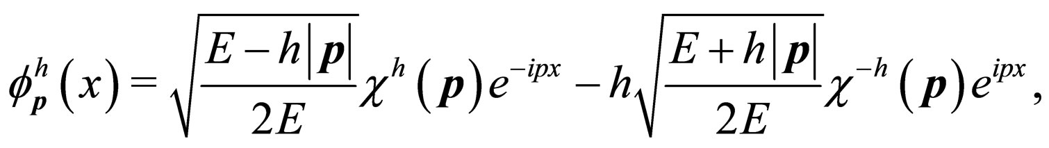 (19)
(19)
with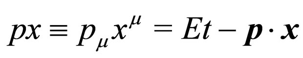 . We observe that Majorana field can be written as superposition of positive and negative energy states.
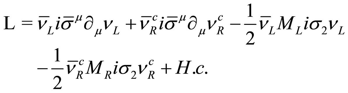
The Lagrangian density which describes a free twocomponent Majorana field is given by
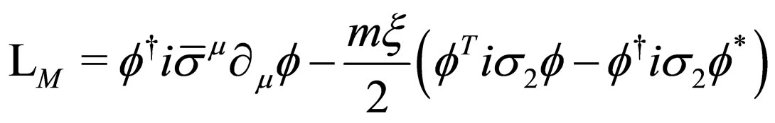 (20)
(20)
where the two-component Majorana field  and its conjugated field
  behave as Grassmann variables. It is very easy to prove that the two-component Majorana Equation (14) can be obtained from the Lagrangian density (20) using the Euler-Lagrange equation. Additionally, we can obtain the following energy-momentum tensor from (20),
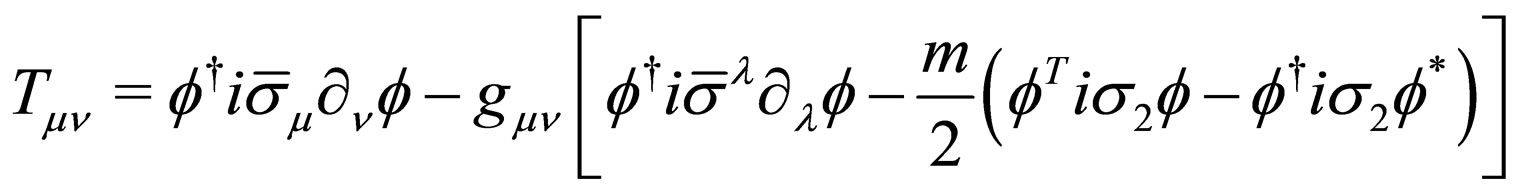 .
.
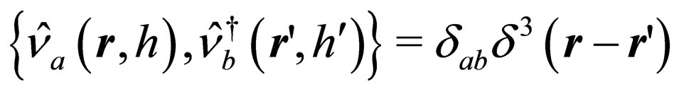
Following the standard canonical quantization procedure, we now consider the Majorana field  and its conjugated field
  as operators which satisfy the usual canonical anticonmutation relations given by
 ,
,
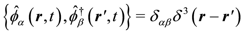 where
where . Using the Heisenberg equation for the Majorana field
 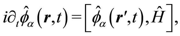 we can obtain its corresponding Majorana Equation (14). By means of the energy-momentum tensor it is possible to prove that the Hamiltonian operator can be written as
 .
.
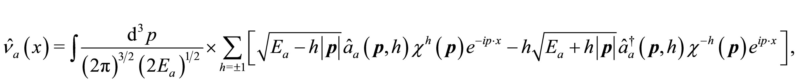
The expansion in a Fourier series for the Majorana field operator is [24-26] (see Equation (21)).
where we have used the free-particle solution (19) and operators ,
,  which satisfy the anticonmutation relations
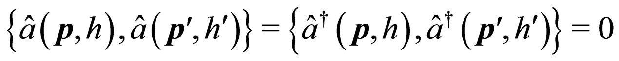 ,
,
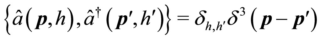 .
.
Then we can identify  as the annihilation operator and
  as the creation operator of a Majorana fermion with momentum
  and helicity h.
3. Masses for Majorana Neutrino Fields
The most accepted way to generate neutrino masses is through the seesaw mechanism. In this section we consider a type I seesaw scenario which leads to get light left-handed neutrinos and heavy right-handed neutrinos. For the case of two neutrino generations, a Dirac-Majorana mass term is given by [29]
 (22)
(22)
where  represents the hermitic conjugate term,
  is the vector of flavor neutrino fields written as
 (21)
(21)
 (23)
(23)
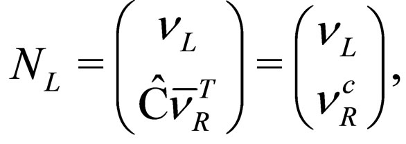
where  represents a doublet of left-handed neutrino fields active under the weak interaction and
  represents a doublet of right-handed Majorana neutrino fields non active (sterile) under the weak interaction. These doublets are given by
 (24)
(24)
In the Dirac-Majorana term (22),  is a
is a  non-diagonal matrix of the form
 (25)
(25)
where ,
,  and
and  are
are  matrixes. The vector of neutrino fields with definite masses
  can be written by mean of a unitary matrix
  as follows
 (26)
(26)
where  has the form
 (27)
(27)
The unitary matrix  is chosen in such a way that the non-diagonal matrix
  can be diagonalized through the similarity transformation
 (28)
(28)
where  is a diagonal matrix which is defined by
 , where
 . The masses of the neutrino fields of definite masses
  are
are , with
 .
.
The seesaw scenario is established imposing the following conditions into the matrix (25):
 ,
,  , thus the matrix
  is diagonalized as
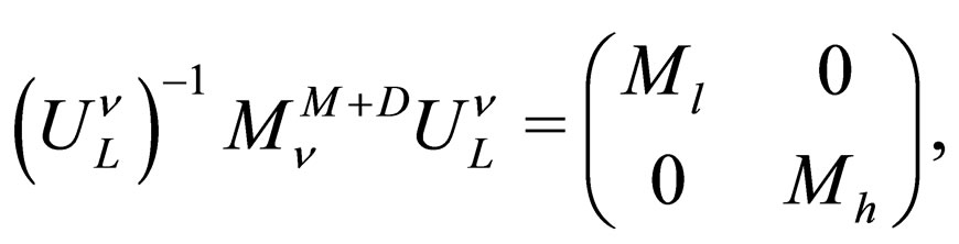 (29)
(29)
where  is the light neutrino mass matrix and
  is the heavy neutrino mass matrix. If the unitary matrix
  is expanding considering terms until of the order
 , the light and heavy neutrino mass matrixes can be written as
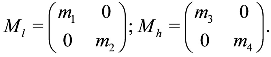 (30)
(30)
The Dirac-Majorana mass term (22) can be written in terms of the neutrino fields of definite masses  as
as
 (31)
(31)
where the matrixes  and
and  are given by (30) and the doublets
  and
and  are written as
 (32)
(32)
The neutrino fields of definite masses  and
and  have associate respectively the light masses
 and
and 
and the neutrino fields of definite masses  and
and  have associate respectively the heavy masses
  and
and , where
 ,
,  are Yukawa couplings,
  is the electron mass and
  is the muon mass.
As it will be shown in the next section, starting from the Dirac-Majorana mass term
 (33)
(33)
where  and
and  are the flavor doublets of non-definite masses given by (24), while
  and
and  are
are  non-diagonal matrixes, it will be possible to obtain the Dirac-Majorana mass term (31) after the diagonalization of the matrixes
  and
and .
.
4. Mass and Flavor Neutrino States
In the next we suppose that the Majorana fields  and
and  describe the active light left-handed neutrinos that are produced and detected in the laboratory, while the Majorana fields
  and
and  describe the sterile heavy right-handed neutrinos which there exist in a type I seesaw scenario.
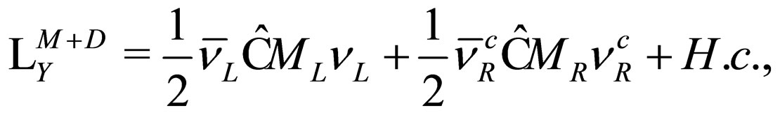
In the Section (2) we have presented a lagrangian density (20) which describes a free Majorana fermion. This lagrangian density can be extended to describe a system of two flavor left-handed neutrinos and two flavor righthanded neutrinos with non-definite masses. Using the Dirac-Majorana mass term given by (33), the lagrangian density describing this system is given by
 (34)
(34)
where the non-diagonal mass matrixes  and
and  are written as
 (35)
(35)
 (36)
(36)
We observe that the form of the matrixes  and
and  is the same. In the next, we will restrict to the lefthanded Majorana neutrinos, but the results are directly extended to the right-handed Majorana neutrinos. From the Euler-Lagrange equations we obtain that the coupled equation of motion for the flavor left-handed neutrino fields
  and
and  are
are
 (37)
(37)
 (38)
(38)
respectively. We observe that flavor neutrino fields are coupled by means of the parameter . With the purpose of decoupling the equations of motion for the flavor left-handed neutrino fields, now we consider the most general unitary matrix
  given by
 (39)
(39)
where the phases  and
and  appear as a consequence of the Majorana condition (7). The definite-mass neutrino field doublet
  given by (32) is related to the flavor left-handed neutrino doublet
  given by (24) by mean of
 (40)
(40)
Without a lost of generality, we can change the phases of the flavor left-handed neutrino fields by means of and
and . Thus there is just a phase
  that can not be eliminated. So the matrix
  can be rewritten as
 (41)
(41)
Now the diagonalization of the mass matrix (35) given by
 (42)
(42)
is valid for
with
 (43)
(43)
and thus the neutrino fields with definite masses  and
and  have respectively the following masses
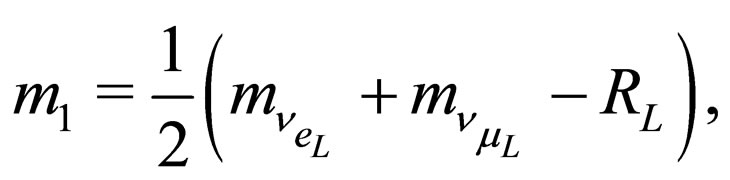 (44)
(44)
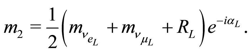 (45)
(45)
We observe that in the expression for  appears the factor
  which suggest that this mass could be complex. However the diagonalization given by (42) is not completely right because
  is a symmetric matrix. So from (42) the diagonalization should be of the form
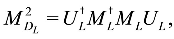 (46)
(46)
where we have considered that this matrix is hermitic, i.e. . So the values
  and
and  are the quadratic roots of the eigenvalues of
 . This last result implies that these eigenvalues can be multiplied by a complex phase.
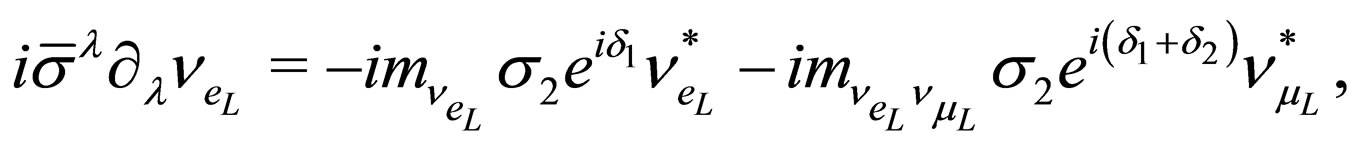
The expression (40) gives the mixing of the flavor neutrino fields in terms of the neutrino fields with definite masses. The neutrino fields with definite masses  and
and  obey Majorana field equations of the form
 (47)
(47)
 (48)
(48)
with the purpose of eliminating the phase  from the last equation of motion, we can make the following phase transformation
 . Now the unitary matrix can be written as
 (49)
(49)
We observe that the phase  was eliminated from the last equation of motion but not from the unitarian matrix
 . So it proves that this phase is physical and should be involved in some processes. This phase could play an important role in the case of doublet beta decay process.
Following a similar procedure for the right-handed Majorana neutrinos, we find that the definite-mass neutrino field doublet  given by (32) is related to the flavor right-handed neutrino doublet
  given by (24) by mean of
 (50)
(50)
where the unitary matrix  is given by
 (51)
(51)
where  is given by
 (52)
(52)
Next we consider the canonical quantization of the neutrino fields with definite mass by stating the anticonmutation relations given by
 ,
,
 and
and
where  represent neutrino mass states. Each one of the definite-mass neutrino field operators
  obeys a Majorana equation. It is possible to expand each one of these field operators on a plane-wave basis set as was shown in (21) (see Equation (53)).
where  is the energy of the neutrino field with definite mass which is tagged by
 .
.
The flavor neutrino field operators tagged by  are defined as superposition of the definite-mass neutrino field operators
  given by (53) through the expression
 (54)
(54)
where U is the unitarian matrix defined by (49) for left-handed neutrinos and by (51) for right-handed neutrinos, meanwhile neutrino flavor states  are defined in terms of the neutrino mass states
  as
as
 (55)
(55)
Thus we have found a relation between neutrino flavor states and neutrino mass states using operator fields. As flavor states are physical states since they could be detected in interaction processes, flavor states are non-stationary. So their temporal evolution gives the probability of transition between them. Therefore, this probability describes Majorana neutrino oscillations studied as follows.
5. Left-Handed Neutrino Oscillations
Now we will focuss our interest in the description of lefthanded neutrino oscillations in vacuum from a cinematical point of view. For this reason we will not consider in detail the weak interaction processes involved in the creation and detection of left-handed neutrinos. However, these processes are manifested when boundary conditions are imposed in the probability amplitude of transition between two neutrino flavor states. We suppose that a neutrino with a specific flavor is created in a point of space-time  as a result of a certain weak interaction process. We will determine the probability amplitude to find out the neutrino with another flavor in a different point of space-time
 . We assume that neutrinos are created under the same production process with different values of energy and momentum. These dynamical quantities are related among themselves under the specific production process.
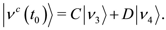
The initial left-handed neutrino flavor state in the production time ( ) corresponds to the following superposition of neutrino mass states
 (56)
(56)
where . Each of these neutrino mass states has associated a specific four-momentum. We assume that in the production point it was created a left-handed electronic neutrino with each massive field having a four-momentum given by
 , with
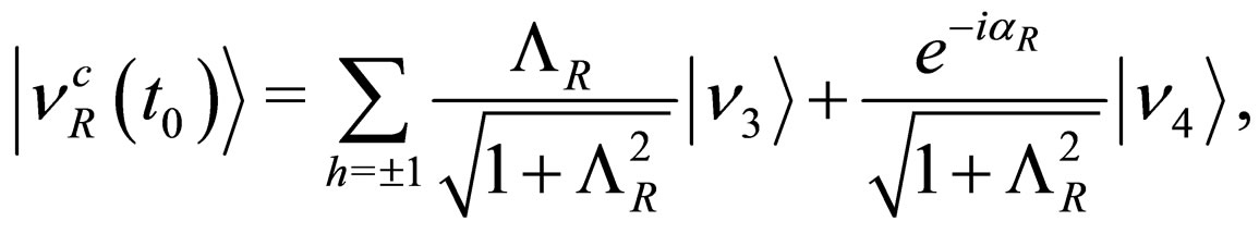
  The initial left-handed electronic neutrino state satisfying the condition
  is written as
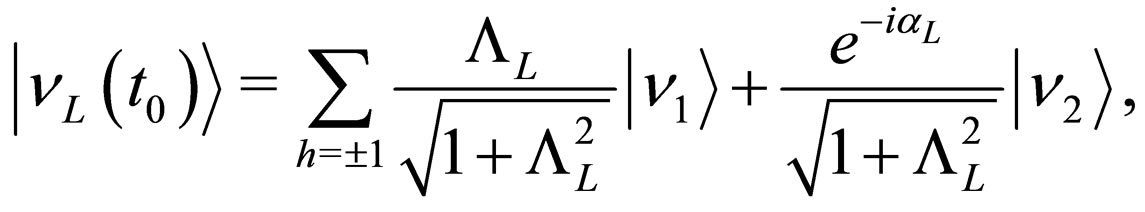 (57)
(57)
where the sum over helicities is taken over the neutrino mass states. This sum over helicities must be considered to describe appropriately the initial left-handed neutrino flavor state because the helicity is a property which is not directly measured in the experiments. The manner as the electronic left-handed neutrino state has been built in the production point is in agreement with the experimental fact that left-handed neutrinos are ultra-relativistic.
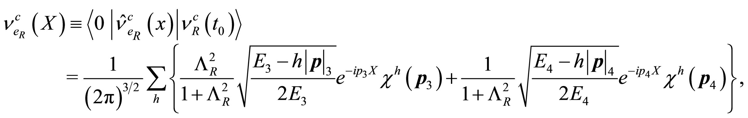
The neutrino mass states involve in the superposition given by (57) are obtained from the vacuum state as
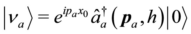
where we have included thephase factor .
.
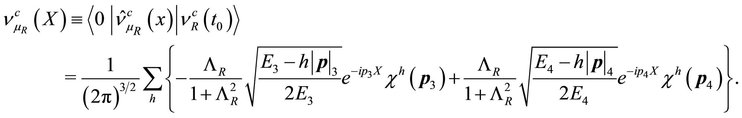
This phase factor gives us information about the fourspace time where the left-handed neutrino was created. The probability amplitudes for transitions to electronic and muonic left-handed neutrinos are respectively given by
 (53)
(53)
 (58)
(58)
 (59)
(59)
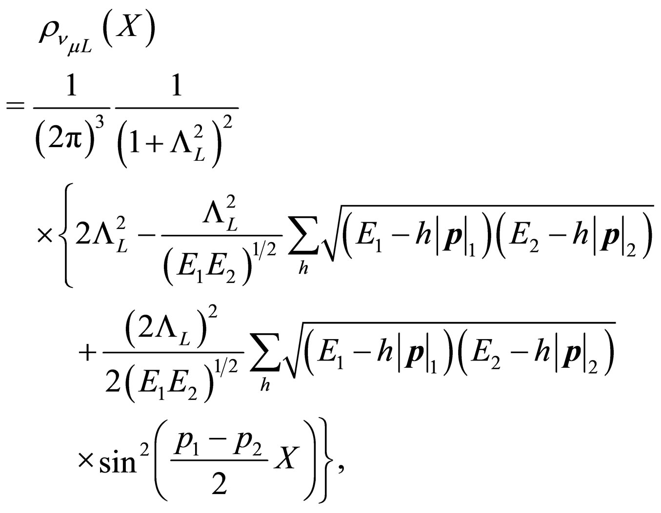
where we have used some expansions over the Majorana fields and we have taken  which corresponds to a four-vector associated to the distance and time of neutrino propagation. The probability densities
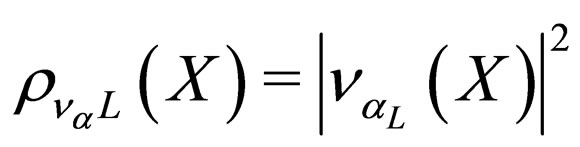
respectively are
 (60)
(60)
 (61)
(61)
where we have taken into account that spinors  and
and  are the same because vectors
  and
and  are co-linear. The probability densities (60) and (61) that we have found present a serious problem. If we fix
  into (60) and (61) we find that
 (62)
(62)
 (63)
(63)
and we observe that the probability density (63) can be different from zero, i.e. it can exist a muonic neutrino in the production point which disagrees with the initial conditions. The origin of this problem is related to the weak state definition (55) that we have used before. As it was previously mentioned into the introduction, the flavor definition (55) is not complectly consistent and it is necessary to define appropriate flavor states [24].
Ultra-Relativistic Limit: Left-Handed Neutrino Oscillations
This problem can be solved by taking an approximation in the probability densities (60) and (61) based on the fact that left-handed neutrinos are ultra-relativistic particles because their masses are very small. Here we consider energy and momentum different for every mass state. In general we can write
 (64)
(64)
 (65)
(65)
where the parameters  and
and  are determined in the production process and E is the energy for the case in which neutrinos were massless. For instance, for the pion decay process we have
 (66)
(66)
 (67)
(67)
where  is the muon mass and
  is the pion mass. Because for the ultra-relativistic limit
 , we can approximate the expressions (64) and (65) to
 (68)
(68)
 (69)
(69)
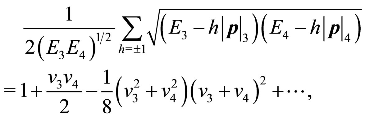
Now it is possible to prove that the right side of the relation
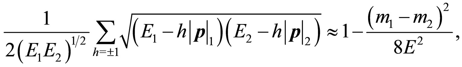 (70)
(70)
can be approximated to the unit because , where
 . On the other hand, neutrino propagation time T is not measured in neutrino experiments [3,9,17]. In this kind of experiments is measured the distance L between the neutrino source and the detector. By this reason, it can be possible to find a analytical expression that establishes a relation between T and the propagation distance
 . In our approach using plane waves, for the ultra-relativistic limit we can write
 (71)
(71)
This relation implies that the propagation distance and the propagation time for neutrinos are approximately equal because in the ultra-relativistic limit a neutrino mass state has a mass too small and its velocity of propagation  is approximately equal to speed velocity
 , i.e.
 . However, a most precise relation between L and T must be described by an expression that should include explicitly the velocities of the two neutrino mass states involved in such a way that this expression for the ultra-relativistic limit should lead to (71).
So for the ultra-relativistic limit the probability densities (60) and (61) can be written as
 (72)
(72)
 (73)
(73)
where we have used  and
and . Under this approximation it is clear that these probability density does not depend from the production process due to that there is no dependence from
 . Thus these probability densities satisfy the boundary conditions that we have imposed.
In the next we will prove that the probability densities (72) and (73) have the form of the standard probability densities for neutrino oscillations. In the context of the standard formalism of neutrino oscillations (assuming CP conservation), for the two generation case considering here, the representation of the unitary matrix  that appears into the expression (40) is given by [30]
 (74)
(74)
where  is the mixing angle. If we compare the unitary matrix given by (49) with the one given by (74), we observe that
  and then it is very easy to obtain that
 (75)
(75)
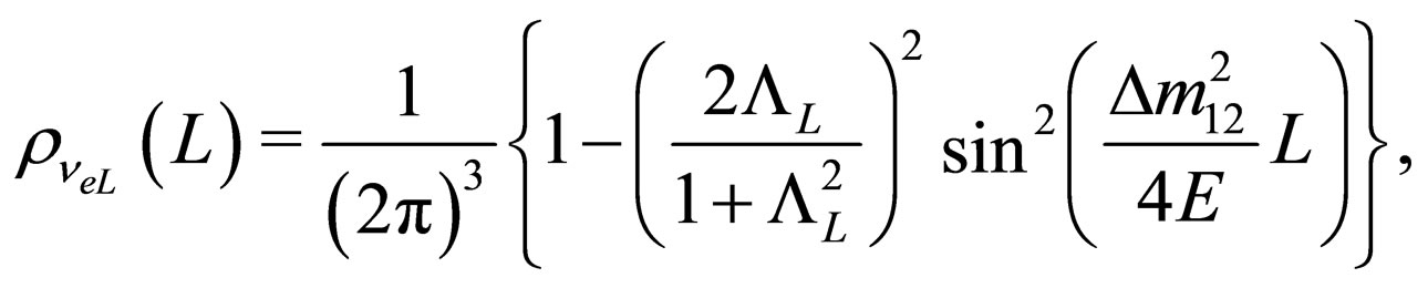
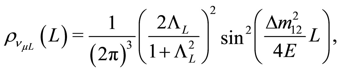
Substituting (75) into (72) and (73), we obtain the expressions
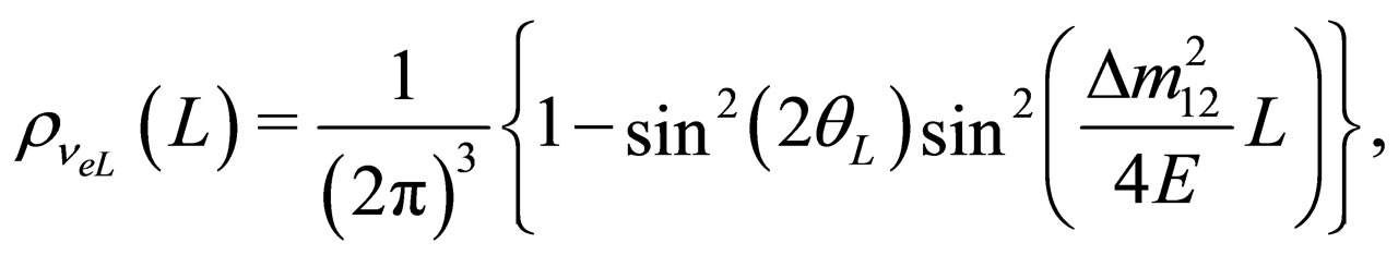 (76)
(76)
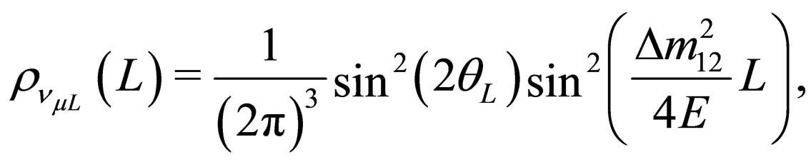 (77)
(77)
which are the standard probability densities for lefthanded neutrino oscillations in the two flavor case [30].
6. Right-Handed Neutrino Oscillations
The initial right-handed neutrino flavor state in the production time ( ) corresponds to the following superposition of neutrino mass states
 (78)
(78)
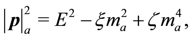
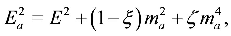
where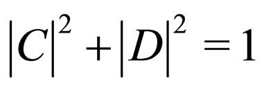 . Each of these neutrino mass states has associated a specific four-momentum. We assume that in the production point it was created a right-handed electronic neutrino with each massive field having a four-momentum given by
 , with
  The initial right-handed electronic neutrino state satisfying the condition
  is written as
 (79)
(79)
where the sum over helicities is taken over the neutrino mass states.
The probability amplitudes for transitions to electronic and muonic right-handed neutrinos are respectively given by
 (80)
(80)
 (81)
(81)
The probability densities 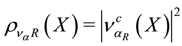 respectively are
 (82)
(82)
 (83)
(83)
where we have taken into account that spinors  and
and  are the same because vectors
  and
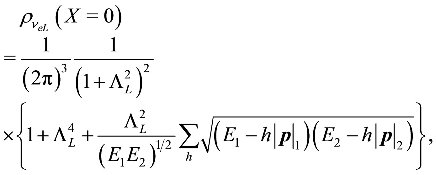
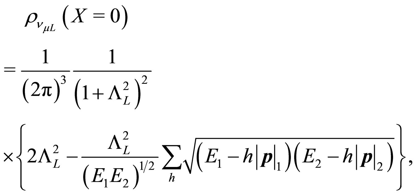
and  are co-linear. The probability densities (82) and (83) that we have found present a serious problem. If we fix X = 0 into (82) and (83) we find that
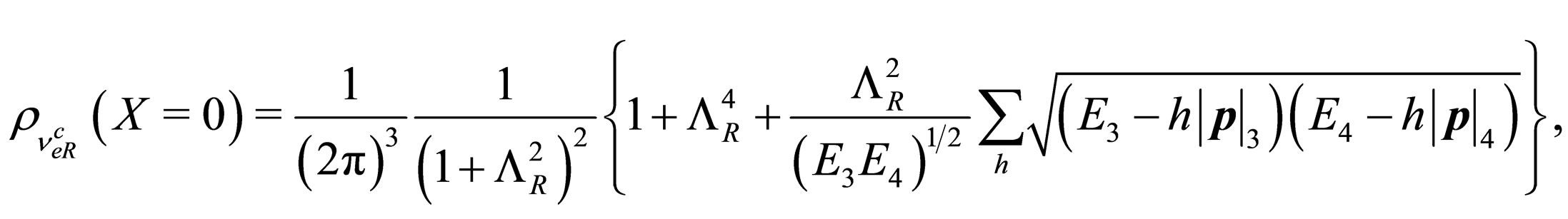 (84)
(84)
 (85)
(85)
and we observe that the probability density (85) can be different from zero.
Non-Relativistic Limit: Right-Handed Neutrino Oscillations
This problem can be solved by taking an approximation in the probability densities (82) and (83) based on the fact that right-handed neutrinos are non-relativistic particles because their masses are very large. By this reason, we take the non-relativistic approximation, i.e.  So we have
 (86)
(86)
Therefore, we suppose that heavy right-handed Majorana neutrinos obey simply the relativistic dispersion relation. So we obtain the following approximation
where the non-relativistic velocity of the neutrino is , meanwhile the phase is approximated to
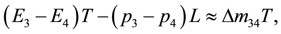 (88)
(88)
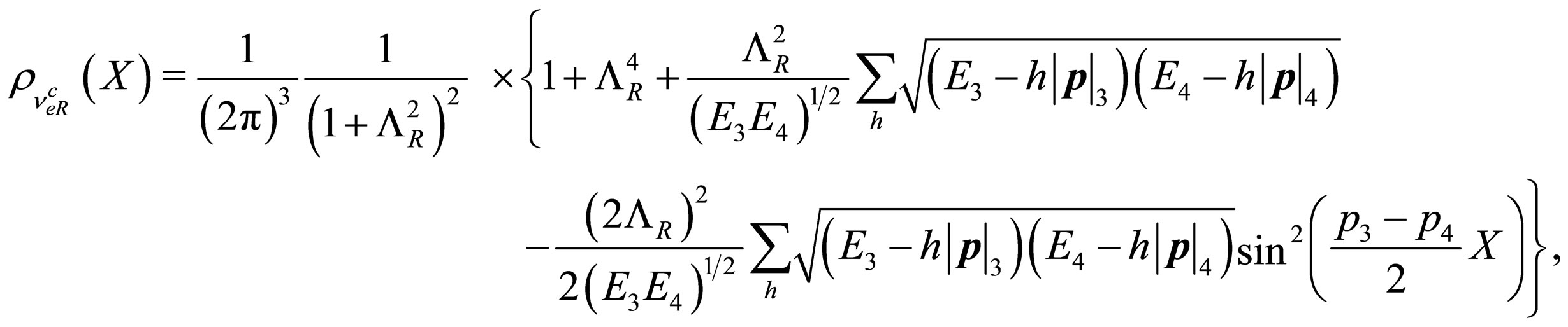
with . So the probability densities of transition are given by
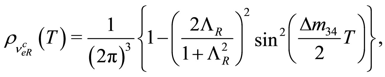 (89)
(89)
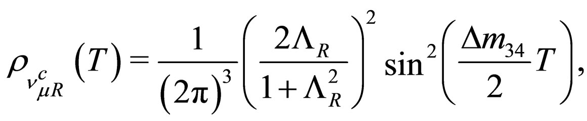 (87)
(87)
where  is given by (52). The last probability densities satisfy the normalization and boundary conditions. Unlikely to the case of left-handed neutrino oscillations described by (60) and (61), the argument of the periodic function for the right-handed neutrino oscillations depends on the linear mass difference
  and the propagation time T. The description of heavy right-handed neutrino oscillations that we present here could be of interest in cosmological problems [31]. As it has been proposed in the literature, heavy-heavy neutrino oscillations could be responsible for the baryon asymmetry of the universe through a leptogenesis mechanism [32-34]. But it should be noted that if the propagation of heavy right-handed neutrinos is considered as superpositions of mass-eigenstate wave packets [25], then the oscillations do not take place because the coherence is not preserved: in other words, the oscillation length is comparable or larger than the coherence length of the right-handed neutrino system [25].
7. Conclusions
In this work we have studied neutrino oscillations in vacuum between two flavor states considering neutrinos as Majorana fermions. We have performed this study for the case of flavor states constructed as superpositions of mass states extending the Sassaroli model which describes Majorana neutrino oscillations by considering neutrino mass states as plane waves with specific momenta. In the context of a type I seesaw scenario which leads to get light left-handed and heavy right-handed Majorana neutrinos, the main contribution of this work has been to obtain in a same formalism the probability densities which describe the oscillations for light lefthanded neutrinos (ultrarelativistic limit) and for heavy right-handed neutrinos (non-relativistic limit). In this work we have performed the canonical quantization procedure for Majorana neutrino fields of definite masses and then we have written the neutrino flavor states as superpositions of mass states using quantum field operators. We have calculated the probability amplitude of transition between two different neutrino flavor states for the light and heavy neutrino cases and we have established normalization and boundary conditions for the probability density. After the ultra-relativistic limit was taken in the probability densities for the left-handed neutrino case lead to the standard probability densities which describe light neutrino oscillations. For the right-handed neutrino case, the expressions describing heavy neutrino oscillations in the non-relativistic limit were different respect to the ones of the standard neutrino oscillations. However, the right-handed neutrino oscillations are phenomenologically restricted as is shown when the propagation of heavy neutrinos is considered as superpositions of mass-eigenstate wave packets [25].
This work establish a framework to study Majorana neutrino oscillations for the case where mass states are described by Gaussian wave packets as will be presented in a forthcoming work [35]. The wave packet treatment is necessary owing to the neutrinos are produced in weak interaction processes without a specific momenta. Additionally the plane wave treatment can not describe production and detection localized processes as occur in neutrino oscillations.
8. Acknowledgements
C. J. Quimbay thanks DIB by the financial support received through the research project “Propiedades electromagnéticas y de oscilación de neutrinos de Majorana y de Dirac”. C. J. Quimbay thanks also Vicerrectoría de Investigaciones of Universidad Nacional de Colombia by the financial support received through the research grant “Teoría de Campos Cuánticos aplicada a sistemas de la Física de Partículas, de la Física de la Materia Condensada y a la descripción de propiedades del grafeno”.
REFERENCES
- E. Majorana, “Teoria simmetrica dell’elettrone e del positrone,” Nuovo Cimento, Vol. 14, 1937, p. 171.
- P. B. Pal and R. N. Mohapatra, “Masive neutrinos in physics and astrophysics,” World Scientific Publishing, Singapore, 2004.
- C. Giunti and Ch. Kim, “Fundamental of neutrinos in physics and astrophysics,” Oxford University Press, New York, 2007.
- K. Nakamura, et al., “Particle Data Group, the review of particle physics,” Journal of Physics G, Vol. 37, 2010, Article ID: 075021.
- A. Bottino, C. W. Kim, H. Nishiura and W. K. Sze, “Model for Lepton Mixing Angles and Majorana neutrino masses,” Physical Review D, Vol. 34, No. 3, 1986, pp. 862-867. doi:10.1103/PhysRevD.34.862
- B. Pontecorvo, “Neutrino experiments and the problem of conservation of leptonic charge,” Soviet Physics— JETP, Vol. 26, 1968, p. 984.
- S. M. Bilenky and B. Pontecorvo, “Lepton mixing and neutrino oscillations,” Physics Reports, Vol. 41, No. 4, 1978, pp. 225-261. doi:10.1016/0370-1573(78)90095-9
- B. Kayser, “On the quantum mechanics of neutrino oscillation,” Physical Review D, Vol. 24, No. 1, 1981, pp. 110-116. doi:10.1103/PhysRevD.24.110
- C. Giunti, C. W. Kim and U. W. Lee, “When Do Neutrinos Really Oscillate? Quantum mechanics of neutrino oscillations,” Physical Review D, Vol. 44, No. 11, 1991, pp. 3635-3640. doi:10.1103/PhysRevD.44.3635
- J. Rich, “The quantum mechanics of Neutrino Oscillations,” Physical Review D, Vol. 48, No. 9, 1993, pp. 4318- 4325. doi:10.1103/PhysRevD.48.4318
- M. Zralec, “From kaons to neutrinos: Quantum mechanics of particle oscillations,” Acta Physica Polonica B, Vol. 29, 1998, pp. 3925-3956.
- E. Sassarolli, “Neutrino oscillations: A relativistic example of a two-level system,” American Journal of Physics, Vol. 67, No. 10, 1999, pp. 869-875. doi:10.1119/1.19140
- M. Blasone and G. Vitiello, “Quantum Field Theory of Fermion Mixing,” Annals of Physics, Vol. 244, No. 2, 1995, pp. 283-311. doi:10.1006/aphy.1995.1115
- E. Alfinito, M. Blasone, A. Iorio and G. Vitiello, “Squeezed neutrino oscillations in Quantum Field Theory,” Physics Letters B, Vol. 362, No. 1-4, 1995, pp. 91-96. doi:10.1016/0370-2693(95)01171-L
- C. Y. Cardall, “Coherence of Neutrino Flavor Mixing in Quantum Field Theory,” Physical Review D, Vol. 61, No. 7, 2000, Article ID: 073006. doi:10.1103/PhysRevD.61.073006
- A. D. Dolgov, “Neutrinos in cosmology,” Physics Reports, Vol. 370, No. 405, 2002, pp. 333-535. doi:10.1016/S0370-1573(02)00139-4
- M. Beuthe, “Oscillations of neutrinos and mesons in Quantum Field Theory,” Physics Reports, Vol. 375, No. 2-3, 2003, pp. 105-218. doi:10.1016/S0370-1573(02)00538-0
- Y. F. Li and Q. Y. Liu, “A Paradox on Quantum Field Theory of Neutrino Mixing and oscillations,” Journal of High Energy Physics, Vol. 2006, 2006, Article ID: 048. doi:10.1088/1126-6708/2006/10/048
- M. Dvornikov and J. Maalampi, “Oscillations of Dirac and Majorana neutrinos in matter and magnetic field,” Physical Review D, Vol. 79, No. 11, 2009, Article ID: 113015. doi:10.1103/PhysRevD.79.113015
- E. Kh. Akhmedova and J. Kopp, “Neutrino oscillations: Quantum Mechanics vs. Quantum Field Theory,” Journal of High Energy Physics, Vol. 2010, No. 4, 2010, p. 8. doi:10.1007/JHEP04(2010)008
- E. Sassaroli, “Flavor oscillations in Field Theory,” http://arxiv.org/abs/hep-ph/9609476v2
- E. Sassaroli, “Neutrino Flavor Mixing and oscillations in field theory,” http://arxiv.org/abs/hep-ph/9805480
- E. Sassaroli, “Two component theory of neutrino flavor mixing,” http://arxiv.org/abs/hep-ph/9710239v1
- C. Giunti, C. W. Kim and U. W. Lee, “Remarks on the Weak States of neutrinos,” Physical Review D, Vol. 45, No. 7, 1992, pp. 2414-2420. doi:10.1103/PhysRevD.45.2414
- C. W. Kim, C. Giunti and U. W. Lee, “Oscillations of Non-Relativistic Neutrinos,” Nuclear Physics B—Proceedings Supplements, Vol. 28, No. 1, 1992, pp. 172-175. doi:10.1016/0920-5632(92)90167-Q
- K. M. Case, “Reformulation of the Majorana theory of neutrino,” Physical Review, Vol. 107, No. 1, 1957, pp. 307-316. doi:10.1103/PhysRev.107.307
- P. B. Pal, “Dirac, Majorana and Weyl Fermions,” American Journal of Physics, Vol. 79, No. 5, 2011, p. 485. doi:10.1119/1.3549729
- E. Marsch, “The Two-Component Majorana EquationNovel Derivations and Known Symmetries,” J. Mod. Phys, Vol. 2, No. 10, 2011, pp. 1109-1114. doi:10.4236/jmp.2011.210137
- S. M. Bilenky and S. T. Petcov, “Massive neutrinos and neutrino oscillations,” Reviews of Modern Physics, Vol. 59, No. 3, 1987, pp. 671-754. doi:10.1103/RevModPhys.59.671
- Ch. W. Kim and A. Pevsner, “Neutrinos in physics and astrophysics,” Harwood Academic Publishers, Basel, 1993.
- S. S. Gershtein, E. P. Kuznetsov and V. A. Ryabov, “Reformulation of the Majorana theory of neutrino,” Physics-Uspekhi, Vol. 40, No. 8, 1997, p. 773. doi:10.1070/PU1997v040n08ABEH000272
- E. K. Akhmedov, V. A. Rubakov and A. Yu. Smirnov, “Baryogenesis via neutrino oscillations,” Physical Review Letters, Vol. 81, No. 7, 1998, pp. 1359-1362. doi:10.1103/PhysRevLett.81.1359
- R. R. Volkas, “Neutrinos in cosmology, with some significant digressions,” Particle Physics and Cosmology: Third Tropical Workshop on Particle Physics and Cosmology—Neutrinos, Branes, and Cosmology, San Juan, 19-23 August 2002, pp. 220-239. doi:10.1063/1.1543502
- A. D. Dolgov, “CP violation in cosmology.” http://arxiv.org/abs/hep-ph/0511213v2
- Y. F. Pérez and C. J. Quimbay, “Temporal dispersion effects of Majorana’s wave packets for neutrino oscillations in vacuum,” reprinted in preparation.