Applied Mathematics
Vol.05 No.17(2014), Article ID:51011,25 pages
10.4236/am.2014.517270
Stratified Convexity & Concavity of Gradient Flows on Manifolds with Boundary
Gabriel Katz
5 Bridle Path Circle, Framingham, MA, USA
Email: gabkatz@gmail.com
Copyright © 2014 by author and Scientific Research Publishing Inc.
This work is licensed under the Creative Commons Attribution International License (CC BY).
http://creativecommons.org/licenses/by/4.0/


Received 18 July 2014; revised 16 August 2014; accepted 2 September 2014
ABSTRACT
As has been observed by Morse [1] , any generic vector field v on a compact smooth manifold X with boundary gives rise to a stratification of the boundary
 by compact submanifolds
 , where
 . Our main observation is that this stratification reflects the stratified convexity/concavity of the boundary
 with respect to the
 -flow. We study the behavior of this stratification under deformations of the vector field
 . We also investigate the restrictions that the existence of a convex/concave traversing
 -flow imposes on the topology of X. Let
 be the orthogonal projection of
 on the tangent bundle of
 . We link the dynamics of the
 -flow on the boundary with the property of
 in X being convex/concave. This linkage is an instance of more general phenomenon that we call “holography of traversing fields”―a subject of a different paper to follow.
Keywords:
Morse Theory, Gradient Flows, Convexity, Concavity, Manifolds with Boundary

1. Introduction
This paper is the first in a series that investigates the Morse Theory and gradient flows on smooth compact manifolds with boundary, a special case of the well-developed Morse theory on stratified spaces (see [2] -[4] ). For us, however, the starting point and the source of inspiration is the 1929 paper of Morse [1] .
We intend to present to the reader a version of the Morse Theory in which the critical points remain behind the scene, while shaping the geometry of the boundary! Some of the concepts that animate our approach can be found in [5] , where they are adopted to the special environment a 3 D-gradient flows. These notions include stratified convexity or concavity of traversing flows in connection to the boundary of the manifold. That concavity serves as a measure of intrinsic complexity of a given manifold
 with respect to any traversing flow. Both convexity and concavity have strong topological implications.
Another central theme that will make its first brief appearance in this paper is the holographic properties of traversing flows on manifolds with boundary. The ultimate aim here is to reconstruct (perhaps, only partially) the bulk of the manifold and the dynamics of the flow on it from some residual structures on the boundary, thus the name “holography”.
In Section 2, for so-called boundary generic fields
 on
on
 (see Definition 2.1), we explore the Morse stratification
 of the boundary
 (see Formula (1) and [1] ), induced by the vector field
 on
on .
.
In Section 3, we investigate the degrees of freedom to change this stratification by deforming a given vector field within the space of gradient-like fields (Theorem 3.2, Corollary 3.2, and Corollary 3.3).
In Section 4, for vector fields on compact manifolds, we introduce the pivotal notion of boundary
 -convexity/
 -concavity,
 (see Definition 4.1). Then we explore some topological implications of the existence of a boundary
 -convex/
 -concave traversing field on
 (see Lemma 4.2, Corollary 4.2, Corollary 4.3, and Corollary 4.4).
Let
 denote the orthogonal projection of the field
 on the bundle
 tangent to the boundary. Occasionally, we can determine whether a given field
 is convex/concave just by observing the behavior of the
 -trajectories on the boundary
 (Theorem 4.1, Theorem 4.2). We view the possibility of such determination as an instance of a more general phenomenon, which we call “holography”. This phenomenon will occupy us fully in a different paper.
The Eliashberg surgery theory of folding maps [6] [7] helps us to describe the patterns of Morse stratifications for traversing 3-concave and 3-convex fields (Theorem 5.1, Conjecture 5.1, and Corollary 5.1).
2. The Morse Stratification

Inspired by [1] , we start by introducing some basic notions and constructions that describe the way in which generic vector fields on a compact smooth manifold interact with its boundary.
Let
 be a compact smooth
 -dimensional manifold with a boundary
 . Let v be a smooth vec- tor field on
 which does not vanish on the boundary
 . As a rule, we assume that X is properly contained in a
 -dimensional manifold
 and that the field v extends to a field
 on
on
 so that
 . In fact, we always treat the pair
 as a germ of a space and a field in the vicinity of the given pair
 .
.
Often we will consider vector fields only with the isolated Morse-type singularities (zeros) located away from the boundary. This means that v, viewed as a section of the tangent bundle , is transversal its zero section. In other words, in the vicinity of each singular point, there is a local system of coordinates
 such that the field v can be represented as
 , where all
 .
.
To achieve some uniformity in our notations, let
 and
and .
.
The vector field v gives rise to a partition
 of the boundary
 into two sets: the locus
 , where the field is directed inward of
 , and
, and , where it is directed outwards. We assume that
 , viewed as a section of the quotient line bundle
 over
over , is transversal to its zero section. This assumption implies that both sets
 are compact manifolds which share a common boundary
 . Evidently,
 is the locus where
 is tangent to the boundary
 .
.
Morse has noticed that, for a generic vector field ν, the tangent locus
 inherits a similar structure in con- nection to
 , as
, as
 has in connection to
 (see [1] ). That is,
 gives rise to a partition
 of
of
 into two sets: the locus
 , where the field is directed inward of
 , and
, and , where it is directed outward of
 . Again, let us assume that v, viewed as a section of the quotient line bundle
 over
over , is transversal to its zero section.
For generic fields, this structure replicates itself: the cuspidal locus
 is defined as the locus where v is tangent to
 ;
;
 is divided into two manifolds,
 and
and . In
. In , the field is directed inward of
 , in
, in , outward of
 . We can repeat this construction until we reach the zero-dimensional stratum
 (see Figure 1 and Figure 2 which depict these strata for fields in
 ).
).
These considerations motivate
Definition 2.1 We say that a smooth field v on
 is boundary generic if:
・
 ,
,
・
 , viewed as a section of the tangent bundle
 , is transversal to its zero section,
・ for each , the
, the
 -generated stratum
 is a smooth submanifold of
 ,
,
・ the field , viewed as section of the quotient 1-bundle
 ,
,
is transversal to the zero section of
 for all
 .
.
We denote the space of smooth boundarygeneric vector fields on
 by the symbol
 .
.

Thus a boundary generic vector field
 on
on
 gives rise to two stratifications:
 (1)
(1)
, the first one by closed submanifolds, the second one―by compact ones. Here
 .
.
For simplicity, the notations “ ” do not reflect the dependence of these strata on the vector field
 . When the field varies, we use a more accurate notation “
 ”.
”.
Remark 2.1. Replacing
 with
with
 affects the Morse stratification according to the formula:

where
 when
when , and
, and
 otherwise.

We will postpone the proof of the theorem below until the second paper in this series of articles (see [8] , Theorem 3.4, an extension of Theorem 2.1 below). There we will develop the needed analytical tools.
Theorem 2.1 Boundary generic vector fields form an open and dense subset
 in the space
 of all smooth fields on
 .
.


Figure 1. The Morse stratification generated by the horizontal field
 on a solid
 bounded by the saddle surface
 .
.

Figure 2. A generic field v in the vicinity of a cusp point on the boundary of a solid
 generates the Morse stratification
 (the left diagram) or the Morse stratification
 (the right diagram).
Definition 2.2 We say that a smooth vector field
 on
on
 is of the gradient type (or gradient-like) for a smooth function
 if:
if:
・ the differential
 and the field
 vanish on the same locus
 ,
,
・ the function
 in
in ,
,
・ in the vicinity of , there exist a Rimannian metric
 on
on
 so that
 , the gradient field of
 in the metric
 .
.

Definition 2.3 A smooth function
 is called Morse function if its differential
 , viewed as a section of the cotangent bundle
 , is transversal to the zero section.

Recall that, for a Morse function
 on a compact
 -manifold X, the critical set

is finite, and each point
 has special local coordinates
 such that
 , where
 for all
 (for example, see [9] ).
Definition 2.4 Let
 be a smooth function and
 its gradient-like vector field. We say that the pair
 is boundary generic if the field
 is boundary generic in the sense of Definition 2.1 and the res- trictions of
 to each stratum
 are Morse functions for all
 .
.

Lemma 2.1 Let
 be a compact smooth manifold, and
 a smooth manifold which is stratified by sub- manifolds
 . Let
. Let
 be the space of smooth maps
 which are transversal to each stratum
 . Put
. Put . Next consider the space
 of pairs
 such that

and
 has the property:
 are Morse functions for all
 . Then
 is open and dense in the
space .
.
Proof. Consider the space , where
 denotes the cotangent bundle of
 . The property
 is equivalent to the property of the section
 of the bundle

to be transversal to each (transversal) intersection of the
 -graph
 with each stratum
 . The latter property defines a open set in
 .
.
In order to validate density of
 in
in , we first perturb a given map
 to make it transversal to each stratum
 , and then perturb a given function
 to make the section
 of
of
 transversal to each manifold
 .
.

Theorem 2.2 The boundary generic1 Morse pairs
 on a compact manifold
 form an open and dense subset in the space of all smooth functions
 and their gradient-like fields
 .
.
Proof. By Theorem 2.1, the boundary generic fields
 form an open and dense set in the space of all fields.
Let
 be a complete flag in
 , formed by subspaces
 of codimension j. In the proof of Theorem 3.4 [8] , for every field
 , we will construct a smooth map
 such that
 . Moreover,
 is transversal to each
 , if and only if,
 is a boundary generic field. The construction of the map
 utilizes high order Lie derivatives
 of an auxiliary function
 as in Lemma 3.1 [8] .
Now the property of boundary generic Morse pairs
 to be open and dense in the space of all pairs follows from Lemma 2.1: just let
 ,
,
 ,
,
 , and
, and
 in that lemma.
For the reader convenience, let us sketch now an alternative argument that establishes just the density of boundary generic Morse pairs
 in the space of all pairs. It does not rely on the construction of the map
 from [8] .
We start with a pair
 where
where
 and
and
 at the points of the set where
 . By a small perturbation of
 , we can assume the
 is a Morse function on
 and
and
 its gradient-like field.
Let
 be a compact regular neighborhood of
 in
in
 so small that
 . By Theorem 2.1, we can perturb
 to a new field
 so that
 is boundary generic in the sense of Definition 2.1 and still
 .
.
For a given , the condition
 defines an open cone in the space of all fields
 , subject to the constraint
 . Therefore
 can be chosen both boundary generic and gradient-like for
 . When
 is fixed, so are the stratifications
 .
.
Next, with
 being fixed, we perturb
 again to a new function
 so that
 and
and
 are Morse functions for all j. The perturbation will be supported in the compact
 . We start
constructing
 inductively first from adjusting it on the 1-manifold
 and then moving sequentially to the strata
 with lower indices j. We pick each perturbation
 so small that the open condition
 is not violated. The existence of the desired
 -th perturbation is based on the fact that Morse functions on a compact manifold
 (in this case, on
 ) form an open and dense subset in
 , the space of all smooth functions on
 , being equipped with the Whitney topology. Note that since
 is tangent
to
 along
along
 and
and , the restriction
 has no critical points in the vi-
cinity of . Thus we need to perturb
 only on a compact subset
 which has an
empty intersection with . This perturbation extends smoothly from
 to
to . Eventually, we reach the upper stratum
 , thus constructing a boundary generic approximation of the given pair
 .
.
All the changes
 of
of , but the first one, we have introduced so far are supported in
 , where
 and
and . This proves that the boundary generic pairs form a dense set in the space of all pairs
 , where
 being a
 -gradient-like field, subject to the constraints:
 , and
, and
 being a Morse function.

For a given Morse pair , we denote by
 the set of critical points of the function
 . For a boundary generic Morse pair
 , the finite critical set
 is divided into two complementary sets: the set
 of positive critical points and the set
 of negative ones (see Figure 3).
Remark 2.2. Note that when , it may happen that
 . However, if a component
 of
of
 is a closed manifold, then
 must have local extrema, in which case
 .
.

Consider a generic field
 and a Riemannian metric
 on
on . We denote by
 the orthogonal projection of the field
 on the tangent space
 . Note that if
 is a gradient field for a function
 in metric
 , then
 is automatically a gradient field for the restrictions
 and
and .
.
Take a smooth vector field
 on a compact
 -manifold
 with isolated singularities
 . We denote by
 the localized index of
 at its typical singular point
 . In a
local chart,
 is defined as the degree of a map
 from a small
 -centered
 -sphere
to the unit
 -sphere. The map takes each point
 to the point
 .
.
We define the “global” index
 as the sum
 .
.
For a generic field
 and a Riemannian metric
 on
on , we form the fields
 on
on
 and define the global index of
 by the formula:

Figure 3. Positive (the left diagram) and negative (the right diagram) singularities of
 on the boundary of a solid
 .
.

Let us revisit the beautiful Morse formulas [1] :
Theorem 2.3 (The Morse Law of Vector Fields) For a boundary generic vector field
 and a Riemannian metric on a
 -manifold
 , such that the singularities of the fields
 are isolated for all
 , the following two equivalent sets of formulas hold:

 (2)
(2)
where
 stands for the Euler number of the appropriate space2.

For vector fields with symmetry, the Morse Law of Vector Fields has an equivariant generalization [10] . Here is its brief description: for a compact Lie group
 acting on a compact manifold
 , equipped with a

-equivariant field , we prove that the invariants
 can be interpreted as taking values in the
Burnside ring
 of the group
 (see [11] for the definitions). With this interpretation in place, the appearance of Formula (2) does not change.
Morse Formula (2) has an instant, but significant implication:
Corollary 2.1 Let
 be a smooth neighborhood of the zero set of a vector field
 on a compact
 -manifold
 . Assume that
 is boundary generic with respect to both boundaries,
 and
and . Then

Remark 2.3. Therefore, the numbers

can serve as “more and less localized” definitions of the index invariant .
.

An interesting discussion, connected to Theorem 2.3, its topological and geometrical implications, can be found in the paper of Gotlieb [12] . The “Topological Gauss-Bonnet Theorem” below is a sample of these re- sults.
Theorem 2.4 (Gotlieb) Let
 be a compact smooth
 -dimensional manifold and
 a smooth map which is a immersion in the vicinity of the boundary
 . Let
. Let
 be a Riemannian metric on
 which, in the vicinity of
 , is the pull-back
 of the Euclidean metric on
 . Consider a generic linear function
 such that the composite function
 has only isolated singularities in the interior of
 . Let
. Let
 be the gradient field of
 3. Assume that
 is boundary generic.
Then the degree of the Gauss map

can be calculated either by integrating over
 the normal curvature
 (in the metric
 ) of the hyper- surface
 , or in terms of the
 -induced stratification

by the formula
 (3)4
(3)4
Example 2.1. Let X be an orientable surface of genus g with a single boundary component. Let
 be an immersion, and let
 ,
,
 and
and
 be as in Theorem 2.4.
Since Ф is an immersion everywhere (and not only in the vicinity of ∂X as Theorem 2.4 presumes), we get that . Thus
 . Then Theorem 2.4 claims that the degree of the Gauss map
 is equal to

Thus, the topological Gauss-Bonnet theorem, for immersions , reduces to the equation
 .
.
So the number of
 -trajectories
 in
in
 that are tangent to
 , but are not singletons (they correspond to points of
 ), as a function of genus
 , grows at least as fast as
 .
.
On the other hand, by the Whitney index formula [13] , the degree of
 can be also calculated as
 , where
 denotes the number of positive/negative self-intersections of the curve
 , and
, and .
.
By a theorem of L. Guth [14] , the total number of self-intersections . Moreover, this lower bound is realized by an immersion
 ! Therefore, for any immersion
 , the total number of self-intersections of the curve
 can be estimated in terms of the boundary-tangent
 -trajectories:

and for some special immersion , we get

Corollary 2.2 Let
 be a compact
 -manifold with boundary, which is properly contained in an
open
 -manifold
 . Let
. Let
 be a smooth map which is a immersion in the vicinity of the
boundary . Let
. Let
 be a Riemannian metric on
 which, in the vicinity of
 , is the pull-back
 of the Euclidean metric on
 .
.
Let
 be a linear function, and
 its composition with the map
 . Form the gradient field
 in
in . Assume that the pair
 is boundary generic in the sense of Definition 2.4.
For each , consider a
 -small tubular neighborhood
 of the manifold
 in
in . Then
 is an immersion. This setting gives rise to the Gauss map
 , defined by the
formula , where
 and
and
 is the unit vector inward normal to
 at
at .
.
Then the degree of the Gauss map
 can be calculated either by integrating (with respect to the

-measure ) over
 the normal curvature
 of the hypersurface
 , or in terms of the

-induced stratum :
:
 (4)
(4)
Proof. We will apply Theorem 2.4 to the field
 in
in
 to conclude that

Since
 in
in ,
,
 , and the last term of this equation reduces to
 .
.

Remark 2.4. Of course, for an odd-dimensional , the Euler number
 , and so is
 . When
 is even-dimensional (i.e.,
 ), the integral in Equation (4) can be expressed in terms of intrinsic Riemannian geometry of the manifold
 , namely, in terms of the Pfaffian
 . The Pfafian is a
 -differential form, whose construction utilizes the curvature tensor on the manifold (see [15] ). So, when
 ,
,

Given a boundary generic field
 on
on , we introduce a sequence of basic degree-type invariants

which are intimately linked, via the Morse Formula (2), to the invariants .
.
We use a Riemannian metric
 on
on
 to produce the orthogonal projection
 of the field
 on the tangent subspace
 .
.
Let
 be the bundle of unit
 -spheres associated with the tangent bundle of the manifold
 . We denote by
 the restriction of the bundle
 to the subspace
 .
.
For each k, consider two fields, the inward normal field
 to
to
 in
in
 and
and , as sections of the sphere bundle
 (remember,
 is tangent to
 along
along
 so that
 along
along !). Assume that the sections ν and
 are transversal in the space
 . This transversality can be achieved by a perturbation of
 (equivalently, by a perturbation of the metric
 ), supported in the vicinity of the singularity locus
 . Indeed, the intersections occur where the field
 is positively proportional to
 , that is, where
 . The later locus is exactly the locus
 . The perturbation does not affect the stratification
 . Assuming the transversality of the intersection, the locus
 is zero- dimensional.
We define the integer
 as the algebraic intersection number of two
 -cycles,
 and
and , in the ambient manifold
 of dimension
 .
.
Lemma 2.2 For a boundary generic field
 on a Riemannian manifold
 , the following formula holds:

Proof. We already have noticed that the intersection set
 projects bijectively under the map
 onto the locus
 , where the component
 of
of
 vanishes and
 points in- ward of
 . It takes more work to see that the sign attached to the transversal intersection point
 is
is , where
 is the index (the localized degree) of the field
 in the vicinity of its singularity
 . Thus
 . By the Morse Formula (2), the claim of the lemma follows.

Corollary 2.3 The integer
 depends only on the singular locus
 of
of
 and on the local indices of its points.

Question 2.1. How to compute
 in the terms of Riemannian geometry and in the spirit of Theorem 2.4 and Corollary 2.2?

For a boundary generic field
 and a fixed metric
 on
on , each manifold
 comes equipped with a preferred normal framing
 of the normal bundle
 : just consider the unitary inward normal field
 of
of
 in
in , then the unitary inward normal field
 of
of
 in
in , being restricted to
 , then the unitary inward normal field
 of
of
 in
in , being restricted to
 , and so on.
Via the Pontryagin construction [16] , this framing
 generates a continuous map
 . Its homotopy class
 is an element of the cohomotopy set
 . If
. If , then we define
 to be the trivial map that takes
 to the base point in
 .
.
Unfortunately, as we will see soon, ! However, when
 , each of the two loci
 is a closed manifold. Then we can apply the Pontryagin construction only to, say,
 to get a map
 . This application leads directly to the following proposition.
Corollary 2.4 Consider a boundary generic vector field
 such that
 and a metric
 , defined in the vicinity of
 in
in . Then these data give rise to continuous map
 .
.
The homotopy class
 is independent of the choice of
 and a homotopy of

within the open subspace of , defined by the constraint
 .
.
In particular, when , we get an element

and when , an element

If , we can interpret
 also as an element of the homotopy group
 .
.

The elements
 and
and
 have another classical interpretation as elements of oriented framed
cobordism set . In fact, the pair
 defines the trivial element in
 . In
. In
contrast, if , then the bordism class
 may be nontrivial.
Let us recall the definition of framed cobordisms (for example, see [17] ). Let
 be oriented closed smooth
 -dimensional submanifolds of a compact
 -manifold
 , whose normal bundles
 and
and
 are equipped with framings
 and
and , respectively.
We say that two pairs
 and
and
 define the same element in
 , if there is a compact
 -dimensional oriented submanifold
 whose normal bundle
 admits a framing
 so that:
1) ,
,
2) the restriction of
 to
to
 coincides with
 , and the restriction of
 to
to
 coincides with
 .
.
Then the Pontryagin construction establishes a bijection , where
 . If
. If
 both sets admit a structure of abelian groups and the bijection
 becomes a group isomorphism.
Now we are in position to explain why . Consider the obvious embedding

We can isotop
 in
in
 to a regular embedding

such that:
1) , and
, and
2) the inward normal field
 is parallel to the factor
 in the product
 .
.
Note that for , all the normal fields
 are preserved under the imbedding
 . So,
. So,
for any , the normal framing
 of
of
 in
in
 extends to a normal framing

of
 in
in . Therefore
 as an element of the framed bordisms of
 . As a
result, when , we get
 in
in
 (equivalently, in
 ).
).
3. Deforming the Morse Stratification
Let
 be a smooth compact
 -manifold with boundary
 . A boundary generic field
 (see Definition 2.1) gives rise to two stratifications (1).
We are going to investigate how the stratification
 changes as a result of deforming the vector field
 .
.
Lemma 3.1 Let
 be a closed submanifold of a manifold
 and
and
 a closed manifold. Consider a family of maps
 such that each
 is transversal to
 . All the manifolds, maps, and families of maps are assumed to be smooth.
Then all the submanifolds
 are isotopic in
 . In particular, the intersections
 and
and
 are diffeomorphic.
Proof. Let
 be the map defined by the family
 . Thanks to the transversality hypothesis,
 is transversal to
 and
and
 is a submanifold of
 whose boundary is

Let
 be a vector field on
 , normal to each codimension 1 submanifold
 in
in . In the construction of
 , we evidently rely on the property of each
 being transversal to
 . Since
 and
and , each w-trajectory that originates at a point of
 must reach
 in finite time. Therefore, employing the w-flow,
 is diffeomorphic to
 , and the
 -image of that product structure in
 defines a smooth isotopy between
 and
and
 in
in . This isotopy extends to an ambient isotopy of
 itself [18] .
Note that these arguments fail in general if ether M or N have boundaries. However, under additional assumptions (such as being t-independent and
 ), the relative versions of the lemma are valid.

Theorem 3.1 The diffeomorphism type of each stratum
 is constant within each path-connected component of the space
 of boundary generic fields.
Proof. If two generic fields,
 and
and , are connected by a continuous path
 , then they can be connected by a path
 such that the dependence of the field
 on
on
 is smooth. The argument is based on the property of generic fields to form an open set in the space of all fields (Theorem 2.1), the smooth partition of unity technique (which utilizes the compactness of manifold
 ), and the standard techniques of approximating continuos functions with the smooth ones.
Thus it suffices to consider a smooth 1-parameter family of vector fields , connecting
 to
to . Since any generic field
 , viewed as a section of the vector bundle
 , is transversal its zero section, we may apply Lemma 3.1 (with
 ,
,
 being the zero section of
 ,
,
 , and
, and ) to conclude that all the submanifolds
 are isotopic in
 .
.
Since each
 divides
 into a pair of complementary domains,
 and
and , and since their polarity ±is determined by the inward/outward direction of
 , which changes continuously with
 , the ambient isotopy of
 (which takes
 to
to ) must take
 to
to . The isotopy
 extends to an isotopy
 .
.
A similar argument applies to lower strata . Indeed, with the isotopy
 that takes
 to
to
 in place, consider the two sections,
 and
and , of the bundle
 , both sections being transversal to the zero section of
 . Applying again Lemma 3.1, we conclude that the loci
 and
and
 are isotopic in
 (recall that these
loci are exactly the transversal intersections of two sections
 and
and
 of
of
 with its zero section).
Again, an isotopy
 that takes
 to
to
 must take
 to
to . The isotopy
 extends to an isotopy
 which preserves the pair
 . So, the pairs
 and
and
 are diffeomorphic via the composite isotopy
 .
.
This reasoning can be recycled to prove that all the pairs
 and
and
 are diffeomorphic via a single isotopy of
 . This argument is carried explicitly in the proof of Theorem 3.4 from [8] .

Corollary 3.1 Let
 be a
be a
 -dimensional compact smooth manifold with boundary.
Within each path-connected component of the space
 of generic fields, the numbers
 , as
, as
well as the numbers , are constant.
Proof. The claim follows instantly from Theorem 3.1 and Lemma 2.2.

For a manifold
 with nonempty boundary, by deforming any given function
 and its gradient-like field
 , we can expel the isolated
 -singularities from
 . This can be achieved by the appropriate “finger moves” which originate at points of the boundary
 and engulf the isolated singularities of
 . The result of these manipulations leads to
Lemma 3.2 Any connected
 -manifold
 with a non-empty boundary admits a Morse function
 with no critical points in the interior of
 and such that
 is a Morse function. Such functions form an open nonempty set in the space
 of all smooth functions on
 .
.
As a result, the gradient-like vector fields
 on
on
 form an open nonempty set in the space
 of all vector fields on
 .
.
Proof. Let us sketch the main idea of the argument. Start with a Morse function . Connect each critical point in the interior of
 by a smooth path to a point on the boundary in such a way that a system of non-intersecting paths is generated. Then delete from
 small regular neighborhoods of those paths (“dig a system of dead-end tunnels”) and restrict
 to the remaining portion
 of
of . Smoothen the entrances of the tunnels so that the boundary of
 will be a smooth manifold which is diffeomorphic to
 . We got a nonsingular function
 on
on . A slight perturbation of
 on
on
 will not introduce critical points in the interior of
 and will deliver a Morse function on its boundary. Indeed, recall that the sets of Morse functions on
 and
and
 are open and dense in the spaces
 and
and
 of all smooth functions, respectively (for example, see [9] ). Of course
 is an open condition imposed on a vector field on a compact manifold. On the other hand, if
 , then any field
 , sufficiently close to
 , will have the property
 . The previous arguments show that the set of gradient-like non-vanishing fields is nonempty. So it is an open nonempty subspace in the space
 of all all vector fields on
 .
.

Eliminating isolated critical points of a given function
 on a manifold with boundary is not “a free lunch”: the elimination introduces new critical points of the restricted function
 . This is a persistent theme throughout our program:
Expelling critical points of gradient flows from a manifold
 leaves crucial residual geometry on its boundary.
This boundary-confined geometry allows for a reconstruction of the topology of .
.
Ideas like these will be developed in the future papers from this series. Meanwhile, the following lemma gives a taste of things to come.
Lemma 3.3 Let
 be a Morse function with no local extrema in the interior of a
 -manifold
 . Then an elimination by a finger move5 of each
 -critical point
 of the Morse index
 results in the introduction of
 new critical points of positive type and
 new critical points of negative type for the modified function
 .
.
Proof. Let
 be a Morse singularity of
 in the interior of
 . Denote by
 a sphere which bounds a
small disk
 centered on
 and such that
 is a Morse function. Without loss of generality, we can
assume that, in the Morse coordinates ,
,
 is given by
 , while
 with all the
 being distinct. Then
 has only Morse-type singularities at the points where the coordinate axes pierce the sphere
 . With respect to the pair
 , these points come in two flavors: positive and negative. The two types are separated by the hypersurface of the cone

In the vicinity of , the intersection
 is exactly the locus

so that the
 -gradient field
 (tangent to
 along
along ) is transversal to
 , the product of two spheres. Therefore, in the vicinity of
 ,
, !
!
The function
 has exactly
 critical points of the positive type and exactly

critical points of the negative type. We shall denote these sets by
 and the two domains in which
 divides
 ―by
―by .
.
Let
 be a local maximum of
 . Note that it is possible to connect
 to a non-singular (for
 ) point
 by a smooth path
 along which f is increasing. Indeed, any non-extendable path
 such that
 either approaches a critical point or reaches the boundary
 . By a small perturbation, we can insure that
 avoids all the (hyperbolic) critical points in the interior of X (by the hypothesis, f has no local maxima/minima in the interior of X). Thus
 can be extended until it reaches the boundary
 at a point
 .
.
Drilling a narrow tunnel , diffeomorphic to the product
 , along
 does not change the topology of X; the function
 retains almost the same list of singularities at the boundary as the function
 has: more accurately, the local maximum at
 disappears in
 and a negative critical point of index 1 of
 appears near the
 -end of the tunnel
 . Thus we have modified f and have eliminated the critical point
 in the interior of X at the cost of introducing on the boundary
 critical points of positive type and
 critical points of negative type.

Soon, motivated by Lemma 3.2, we will restrict our attention to nonsingular functions
 and their gradient-like fields
 ―an open subset in the space of all gradient-like pairs
 ; but for now, let us investigate a more general case.
Consider Morse data , where the field
 is nonsingular along the boundary
 . Extend
 to
to
 and
and , where C is some external collar of
 so that the extension
 is nonsingular in C. At each point
 , the
, the
 -flow defines a projection
 of the germ of
 into the germ of the hypersurface
 .
.
Let
 and
and
 denote the pure strata
 and
and , respectively. At the points
 ,
,
 is a surjection; at the points of
 , it is a folding map; at the points
 , it is a cuspidal map. Often we will refer to points
 by the smooth types of their
 -projections.
As the theorem and the corollary below testify, for a given function , we enjoy a considerable freedom in changing the given Morse stratification
 by deforming the
 -gradient-like field
 (cf. Section 3 in [5] ).
Theorem 3.2 Let
 be a compact smooth
 -manifold with nonempty boundary. Take a smooth function
 with no singularities along
 , and let
 be its gradient-like field. Consider a stratification

of X by compact smooth manifolds , and let
 and
and
 denote the critical sets of the restrictions
 and
and , respectively. Assume that the following properties are satisfied:
・
 ,
,
・
 and
and
 are regular embeddings for all
 ,
,
・ for each
 the functions
 and
and
 have Morse-type critical points at the loci
 and
and , respectively,
・ at the points of ,
,
 and, at the points of
 ,
,
 , where
 is the inward normal to
 in
in
 6.
6.
Then, within the space of
 -gradient-like fields, there is a deformation of
 into a new boundary generic gradient-like field
 , such that the stratification
 , defined by
 , coincides with the given
stratification .
.
Proof. We pick a Riemannian metric g in a collar U of
 in X so that
 becomes the gradient field of f. Consider auxiliary vector fields
 , where
 denotes the orthogonal projection of
 on the tangent spaces of closed manifold
 .
.
The construction of the desired field
 is inductive in nature, the induction being executed in increasing values of the index
 . Figure 4 illustrates a typical inductive step.
Assume that
 has been already constructed so that
 and
and
 for all
 . This assumption implies that
 is tangent to
 exactly along its boundary
 for all
 . Along
 (and thus along
 ), we decompose
 as
as , where
 .
.
The idea is to modify
 in the direction normal to
 in
in , while keeping the rest of its components
 unchanged.
Denote by
 the tangent space of
 at
at . Let
. Let
 be the open half-space of
 positively

Figure 4. Changing the polarity of a typical point from
 to the opposite (to a point of
 ) by deforming the given field
 into the field
 .
.
spanned by the vectors that point inside of . Let
. Let
 be half of the tangent space
 , defined by
 , where
 . We introduce the complementary to
 and
and
 open half-spaces
 and
and .
.
At each point , consider the open cone
 and, at each point
 , the open cone
 (see Figure 4). These cones are non-empty, except perhaps at the points of
 , where
 is anti-parallel to the inward normal
 of
of . However, at
 ,
,
 , and at
 ,
,
 due to the last bullet in the hypotheses of the theorem. Thus, for each
 , there is a number h so that the vector
 (this conclusion uses the the property
 on the set
 ). Similarly, for each
 , there is a number h so that
 . By the partition of unity argument, which employes convexity of the cones
 , there is a smooth function
 which delivers the desired field uk along
 . In order to insure the continuity of h and
 across the boundary
 , we require
 . Thus
 on
on .
.
Put . Now,
 for all
 (these strata depend on the
 ’s only),
and
 by the construction of
 . Moreover,
 for all
 . In fact,
 is tangent to
 along
along . Note that this inductive argument should be modified for
 since
since
 is 0-dimensional.
We smoothly extend
 into a regular neighborhood V of
 in X. Abusing notations, we denote this extension by
 as well. The neighborhood
 is chosen so that there
 .
.
To complete the proof of the inductive step , we form the field
 , where the functions
 deliver a smooth partition of unity subordinate to the cover
 of X. Since
 defines a convex cone in the space of vector fields,
 is a f-gradient-like field with the desired Morse stratification.

Theorem 3.2 has an immediate implication:
Corollary 3.2 Let
 be a Morse function and
 its boundary generic gradient-like field with the
Morse stratification . Assume that compact codimension zero submanifolds
 are chosen so that, for each
 ,
,
 and
and .
.
Then, within the space of f-gradient-like fields, it is possible to deform
 into a new gradient-like boundary generic field
 , such that the stratification
 coincides with the given stratification
 .
.
Moreover, .
.
In particular, if , the claim is valid for any stratification
 as above that terminates with
 .
.

The next proposition (based on Corollary 3.2) shows that, for a given Morse function , by an appropriate choice of gradient-like field
 , the Morse stratification
 can be made topologically very simple and regular: namely, each stratum
 is a disjoint union of
 -dimensional disks. Moreover, when the boundary
 is connected and
 , each stratum
 is a just a single disk.
Corollary 3.3 Let
 be a Morse function on a compact
 -manifold
 ,
,
 being nonsingular along the boundary
 . We divide the connected components
 of the boundary into two types, A and B. By definition, for type A, the singularity set
 , and for type B,
 .
.
Then any f-gradient-like field
 can be deformed, within the space of f-gradient-like fields, into a boundary generic field
 so that, for each component
 of type A and all
 , the stratum
 is diffeomorphic to a disk
 . At the same time, for the components of type
 and all
 , the stratum
 .
.
For the components of type , in contrast, the 1-dimensional stratum
 is a finite union of arcs residing in the circle
 . Moreover,
 , the number or arcs in
 , and the number of points in
 are linked via the formula

, where is the index of the field
 , and
, and
 is the number of boundary components of type
 .
.
Proof. If , for each type A connected component
 of
of , the singularity set
 can be included in a disk
 . By Corollary 3.2, we can deform
 to a new
 -gradient-like field
 , so that the new stratum
 . If
. If , then the singularity set
 can be incapsulated in a disk
 . By the same token, after still another deformation
 of
of , we can arrange for
 and
and . This process repeats itself, unless the dimension of
 becomes one. At its final stage,
 consists of several arcs which are contained in the circle
 .
.
For each type
 connected component
 of
of , by a similar reasoning, we can arrange for
 . Thus,
 for all
 and
and .
.
Therefore, letting
 for all
 in Corollary 3.2, we have established all the claims of the corollary, but the last one.
Since
 and
and
 both are the gradient-like fields for the same Morse function
 , their indexes,
 and
and , are equal. Thus we get

, where
 is the contribution of all the disk-shaped strata
 to the Morse Formula (2).
Recall that, by Corollary 4.4 [5] , for any 3-fold
 and a boundary generic field
 on it, we get
 , provided
 . Thus, as a positive
 increases, the boundary of the disk
 becomes more “wavily”.
For example, by attaching many 2-handles to the boundary of a 2-disk, we get a 2-fold X with a big value
 of
of . On such
 ,
,
 for any gradient-like field
 such that
 .
.
These examples motivate the following question.
Question 3.1 For boundary generic gradient-like fields
 with a fixed value
 of the index
 and a
and a
disk-shaped stratification
 as in Corollary 3.3, what is the minimum
 of
of ?
?

Evidently, such number
 is an invariant of the diffeomorphism type of
 . It seems that
 is semi-additive under the connected sum operation: that is,

4. Boundary Convexity and Concavity of Vector Fields
We are ready to introduce pivotal concepts of the stratified convexity and concavity for smooth vector fields on manifolds with boundary.
Definition 4.1 Given a boundary generic vector field
 (see Definition 2.1), we say that
 is boundary
 -convex, if
 . In particular, if
 , we say that
 is boundary
 -convex, or just boundary convex.
We say that
 is boundary s-concave, if
 . In particular, if
 , we say that
 is boundary 2-concave, or just boundary concave.

Example 4.1. Assume that a compact manifold X is defined as a 0-dimensional submanifold in the interior of a Riemannian manifold , given by an inequality
 , where
 is a smooth function with 0 being a regular value. Then the boundary convexity of a gradient field
 in X can be expressed in terms of the Hessian matrix
 by the inequality

at all points , where
 is tangent to
 . If
. If

, where
 is tangent to
 , then the field
 is boundary concave.

Example 4.2. According to the argument in Lemma 3.3, the complement to a small convex (in the Morse coordinates) disk, centered at a Morse type
 -critical point, is boundary concave with respect to the gradient field
 . In fact, the field
 is both boundary 3-concave and 3-convex! So, if
 is a Morse function on a closed manifold Y with a critical set
 , then the complement X in Y to a small locally convex neighborhood of
 admits a boundary concave
 -gradient-like field (with
 )!
)!

Theorem 4.1 below belongs to a family of results which we call “holographic” (see also and Theorem 4.2). The intension in such results is to reconstruct some structures on the “bulk”
 (or even the space
 itself) from the appropriate flow-generated structures (“observables”) on its boundary
 . A paper from this series will be devoted entirely to the phenomenon of holography for nonsingular gradient flows.
In Theorem 4.1, we describe how some boundary-confined interactions between the critical points of a given function
 of opposite polarities can serve as an indicator of the convexity/concavity of the gradient field
 in X (recall that the convexity/concavity properties of the
 -flow do require knowing the field in the vicinity of
 in X!).
Theorem 4.1 Let ,
,
 be Morse functions and
 and
and
 their gradient fields with respect to a Riemannian metric
 on X and its restriction to
 , respectively. Assume that
 is boundary generic.
If , then there is no ascending
 -trajectory
 , such that

(both critical sets
 depend only on
 ).
).
Conversely, if for a given
 -gradient pair
 , no such
 -trajectory
 exists, then one can deform
 to a new boundary generic pair
 of the
 -gradient type so that
 . Moreover, the fields
 and
and
 on
on
 can be chosen to be arbitrary close in the
 -topology.
In particular, if
 (as sets), then X admits a boundary generic and convex f-gradient-like field
 ; similarly, if
 , then X admits a boundary generic and concave f-gradient-like field
 .
.
Proof. First consider the convex case, that is, the relation between the property
 and the absence of an ascending
 -trajectory
 which connects
 to
to .
.
Consider the function , defined via the formula
 , where
 denotes a unitary field inward normal to
 in
in . Since
 is boundary generic, zero is a regular value of
 . Then

and .
.
If an ascending
 -trajectory
 , which links
 with
with , does exist, it must cross somewhere the boundary
 of
of . Since the field
 is an orthogonal projection of
 on
on , the two fields must agree at any point
 ―the locus where
 is tangent to
 . Thus,
 is the gradient of
 at
at . Therefore, as
 crosses from
 into
into
 at
at , in its vicinity, the arc
 lies below the arc
 (see Figure 5). By the definition of the locus
 , such crossing
 belongs to
 . Therefore,
 , contrary to the theorem hypothesis.
On the other hand, if no such
 -trajectory
 exists, then we claim the existence of a codimension one closed submanifold
 , which separates
 in two manifolds,
 and
and

 , such that the vector field
 , or rather its perturbation
 , is transversal to
 and points outward of
 . Indeed, for each critical point
 , in the local Morse coordinates
 on
on , consider a small closed

-disk
 centered on the critical point x. Denote by
 the closure of the union of downward trajectories of the
 -flow passing through the points of
 (see Figure 6, the left diagram). Let
 be the union
 (see Figure 6, the right diagram).
Since we assume that no descending
 -trajectory
 links a point of
 to a point of
 , we can choose
the disks
 so small that the set
 belongs to the complement
 .
.
For each , the zero cone
 of the Morse function
 separates the sphere
 into two handles,
 and
and
 (each being a product of a sphere with a disk). We denote by
 the handle in
 whose spherical core is formed by the intersection of the unstable disk through
 with the sphere
 . Then, by definition, the set
 is a collection of downward trajectories through the points of
 union with
 . Note that the downward trajectories from a different set
 could enter the disk
 only through the complementary handle
 in its boundary. As a result,
 is a manifold whose piecewise smooth boundary could have corners (see Figure 6, the right diagram). Similarly,
 is a domain in
 whose boundary is piecewise smooth manifold with corners.
Since
 consists of the downward trajectories of
 , if
, if , then any point
 which can be reached from
 following the field
 (for short, “is below
 ”) belongs to
 as well. Therefore the boundary
 is assembled either from downward trajectories or from singletons; the singletons are contributed by some portions of
 where
where
 points outside of the relevant disk
 . Thus either
 is tangent to
 , or it points outside
 .
.
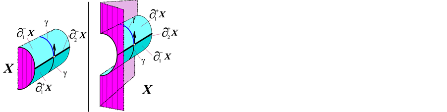
Figure 5. The behavior of a gradient field
 in the vicinity of a point from
 (the left diagram) and in the vicinity of a point from
 (the right diagram), as perceived by an observer moving along the
 -trajectory
 .
.

Figure 6. The set
 (the left diagram) and the set
 (the right diagram).
Away from ,
,
 is of the
 -gradient type. Thus, in each tangent space
 , where
 , there is an open cone
 comprised of
 -gradient type vectors, and
 . Therefore, in the vicinity of
 , we can perturb
 to a new field
 of the
 -gradient type, so that
 points strictly outside
 and still
 for all
 . It is possible to smoothen the boundary
 so that, with respect to a new smooth boundary
 , the field
 still points outside
 , the new domain bounded by
 , and
, and
 for all
 .
.
Note that if , then
 can serve as a separator.
Let
 and
and . With the separator
 in place, consider a smooth function
 with the properties:
1) zero is a regular value of , and
, and ,
,
2) ,
,
 ,
,
3)
 in a neighborhood of
 ,
,
4) , where
 is the inward normal to
 in
in .
.
Note that the field
 points inside of
 along
along
 and outside of
 along
along . It also points outside of
 along
along . As a result, we conclude that
 and
and ; in other words,
 is boundary convex. Note that
 can be chosen arbitrary close to
 . Ineeded, employing Theorem 3.2, we can perturb
 to insure its genericity with respect to the pair
 , and thus the boundary genericity of
 itself.
The argument in the concave case, which deals with the relation between the property
 and the absence of an ascending
 -trajectory
 , connecting
 to
to , is analogous. We just need to switch the polarities of the relevant sets.

Now we need to introduce a number basic notions to which we will return on many occasions in the future.
Definition 4.2 Let
 be a differential
 -form on a manifold
 .
.
We say that a path
 is
is
 -positive (
 -negative), if,
 for all values of the parameter
 .
.

Definition 4.3 Let
 be a closed differential 1-form on a manifold
 , equipped with a Riemannian metric
 . We say that a vector field
 on
on
 is the gradient of
 (and denote it “
 ”), if
 for any vector field
 on
on .
.

Definition 4.4 Let
 be a differential 1-form on a manifold Y and let
 be the set of points
 , where
 is the zero map. Assume that
 for some smooth function
 in the vicinity of
 .
.
We say that a vector field
 is of
is of
 -gradient type if
 on
on
 and
and
 in the vicinity of
 . Here
 is some Riemannian metric in the vicinity of
 (cf. Definition 2.2).

We are in position to formulate a generalization of Theorem 4.1 for closed differential
 -forms―another instance of somewhat weaker “holographic phenomenon”, this time for fields which may not be gradient-like globally.
Theorem 4.2 Let
 be a closed 1-form on a compact manifold
 , equipped with a Riemannian metric
 . Assume that
 and
and
 have only Morse-type singularities. Let the gradient
 be a boundary
generic field, and let .
.
If , then there is no
 -ascending
 -trajectory
 , such that

Assume that there exists a codimension one submanifold , which separates
 and
and
 and such that the field
 is transversal to
 and points outwards/inwards of the domain in
 that is bounded by
 and contains
 . Then one can deform the
 -gradient vector fields
 to a new boundary generic pair
 of the
 -gradient type so that
 .
.
Proof. The
 -gradient fields
 on
on
 are characterized by the property
 , valid on the
locus where . Usually, in this setting, we do not have a natural choice for the wall
 which would separate the singularities of opposite polarities
 and
and
 and such that the field
 would be transversal to N. It seems unlikely that the absence of an ascending
 -trajectory which links
 with
with
 is sufficient to guarantee the existence of a separator N. However, in the presence of such separator N, the arguments are identical with the ones employed in the proof of Theorem 4.1.

Remark 4.1. In Theorem 4.1 and Theorem 4.2, the partition
 of the singular set
 must satisfy some basic relations:


These relations reflect the fact that
 when
when , and
, and
 when
when .
.

Given a metric
 on a Riemannian
 -manifold
 , let us recall a definition of the Hodge Star Operator
 (see [19] ).
Pick a local basis
 of 1-forms in
 and consider the associated basis

of , where
 and the symbol “
 “ stands for omitting the
 -th form
 from the product
 .
.
Assume that, in the dual to
 basis
basis
 of
of , the metric
 is locally given by a matrix
 . Then the matrix
 of the
 -operator in the bases
 ,
,
 is given by the formula
 (5)
(5)
whence .
.
Definition 4.5 A closed differential 1-form
 on a compact manifold Y is called intrinsically harmonic if there exists a Riemannian metric g on Y such that the form
 is closed.

Example 4.3. Let
 be a closed smooth manifold and
 a smooth map with isolated Morse-type singularities. Consider the closed
 -form
-form , the pull-back of the canonic 1-form
 on the circle
 . Assume that one of the
 -fibers,
 , is connected. Then
 is intrinsically harmonic [20] .

Let
 denote the singularity set of a closed 1-form
 on a compact manifold Y. We assume that
 .
.
By Calabi’s Proposition 1 [19] ,
 is intrinsically harmonic if and only if through every point
 there is a
 -positive path
 which either is a loop, or which starts and terminates at the boundary
 .
.
Theorem 4.3 Let
 be a closed
 -form on a Riemannian manifold
 , such that
 . Assume that
 , the restriction of
 to
to , is a harmonic form7.
Then the gradient field
 is not boundary convex or boundary concave (that is,
 and
and ). Thus, if
 is connected, then
 .
.
Proof. We abbreviate
 to
to
 and
and
 to
to . Here
 is the *-operator on the boundary of X
with respect to the given Riemannian metric
 on
on .
.
If
 is a closed
 -form on
 , then by the Stokes Theorem,

However, for a concave/convex gradient field , the
, the
 -form
-form , being restricted to
 , is proportional to the volume form of
 with negative/positive functional coefficient. Indeed, at the points of
 , the angle between
 and the normal
 to
to
 in
in
 is acute, while it is obtuse at the
points of . Therefore,
 when either
 or
or . The resulting contradic-
tion proves that
 and
and .
.
Therefore, when
 is connected, then
 and
and
 must share the common nonempty boundary
 ―the gradient field
 must have cuspidal points.

Example 4.4. Let
 be a compact smooth manifold and
 a smooth map with isolated Morse- type singularities. Consider the closed
 -form
-form , the pull-back of the canonic 1-form
 on the circle
 . Assume that one of the fibers of the map
 is connected. Then there exists a metric

on
 such that the form
 is harmonic ([19] [20] ). Consider the gradient field
 .
.
Then by Theorem 4.3,
 and
and
 for any metric
 that “harmonizes”
 .
.

Definition 4.6 A non-vanishing vector field
 on a compact manifold
 is called traversing if each
 -trajectory is either a closed segment or a singleton which belongs to
 .
.

Remark 4.2. The definition excludes fields with zeros in
 (they will generate trajectories that are homeomorphic to open or semi-open intervals) and fields with closed trajectories. Note that all gradient-like fields of nonsingular functions are traversing, but the gradient-like fields of nonsingular closed 1-forms may not be traversing!

Lemma 4.1 Any traversing vector field is of the gradient type.
Proof. Let
 be a traversing field on X. We extend the pair
 to a pair
 so that X is properly contained in
 and
and .
.
Then every
 -trajectory
 has a local transversal compact section
 of the
 -flow. We can choose
 to be diffeomorphic to a n-dimensional ball with its center at the singleton
 . We denote by
 the union of
 -trajectories through
 .
.
For each
 -trajectory
 , there exists a section
 so that the set
 contains a compact cylinder
 , where
 are positive constants (which depend on
 ), with the properties:
1) ,
,
2) for any
 -trajectory
 through
 , the intersection
 is a segment,
3) the point
 belongs to the interior of segment
 .
.
Then the collection
 forms a cover of
 . Since
 is compact, we can choose
a finite subcover
 of
of .
.
For each
 and the corresponding section
 , we produce a smooth function
 by integrating the vector field
 and using
 as the initial location for the integration.
More accurately, let

be the parametrization of a typical trajectory
 , such that

for all
 and
and
 . This bijective parametrization introduces a smooth product structure

by the formula
 .
.
We define a smooth function
 by the formula
 and denote it (quite appropriately)
by the symbol
 .
.
Let
 be a smooth non-negative function that vanishes only on the boundary
 . Let
. Let
 denote the composition of the
 -directed projection
 with the function
 . Since
 vanishes on
 , the function extends smoothly on X to produce a smooth function
 with the support in
 .
.
Now consider the smooth function
 (6)
(6)
It is well-defined on X. Let us compute its -directional derivative:
 (7)
(7)
Let us explain Formula (7). By the very definition of
 , it is constant on each
 -trajectory, so that
 . Also,
 in
in
 . At the same time,
 , since
 and
and
 increases in the direction of
 . Finally, each
 belongs to the interior of some set
 .
.
Therefore,
 , so that
 is a gradient-like field for
 .
.

Corollary 4.1 Let X be a smooth compact manifold with boundary. Then
 ―the space of traversing vector fields on X―is nonempty and coincides with the intersection
 , where
 denotes the space of gradient-like fields, and
 the space of all non-vanishing fields on X.
Proof. By definition, any traversing field
 on X does not vanish. By Lemma 4.1,
 must be of the gradient type. Thus

On the other hand, for a compact X with a gradient-like
 , each
 -trajectory
 through
 must reach the boundary in both finite positive and negative times (since it is controlled by some Lyapunov function f).
As a result,

It remains to show that
 . By Lemma 3.2,
 , which implies that
 .
.

There are simple topological obstructions to boundary convexity of any gradient-like nonvanishing field on a given manifold X. The next lemma testifies that the existence of boundary convex traversing fields
 imposes severe restrictions on the topology of the manifold X.
Lemma 4.2 A connected
 -manifold X admits a boundary convex traversing8 field
 , if and only if, X is diffeomorphic to a product of a connected compact n-manifold and a segment, the corners of the product being smoothly rounded.
Proof. Indeed, if such convex
 exists,
 must be a deformation retract of X: just use the down flow to produce the retraction. Therefore, when
 , then X is homeomorphic to the quotient space
 , where the equivalence relation “
 ” is defined by collapsing each segment

to a point. If we round the corners generated in the collapse, we will get a diffeomorphism between X and the “lens”
 (see Figure 7).
On the other hand, any product
 , whose conners
 being rounded, admits a field of the desired boundary convex type.

Corollary 4.2 For all
 , any smooth compact contractible
 -manifold X, which admits a boundary convex traversing field, is diffeomorphic to the standard
 -disk.

Figure 7. The existence of a traversing boundary convex field
 (the constant vertical field) on a (n + 1)-manifold X (the ellipsoid-bounded solid) implies that topologically it is a product of a compact n-manifold Y (the elliptical shadow) with an interval.
Proof. By Lemma 4.2, X is diffeomorphic to a product of a fake
 -disk Y with
 , the corners of the product being rounded.
For
 , by Perelman’s results [21] [22] , Y is diffeomorphic to the standard 3-disk. Thus X is diffeomorphic to the standart 4-disk.
For
 , we do not know whether Y is a standard 4-disk.
For
 , the h-cobordism theorem [23] implies that any fake n-disk is diffeomorphic to the standard disk.
This leaves only the case of 5-dimensional X wide open.

We notice that
 is an obstruction to finding boundary convex traversing
 on a
on a
 -dimensional manifold
 with a connected boundary.
Corollary 4.3 Let X be a smooth connected compact
 -manifold with boundary, which admits a boundary convex traversing field.
If
 , then X is diffeomorphic to the product
 , where Y is a closed manifold.
In particular, no connected X with boundary
 , whose number of connected components differs from two, and with the property
 admits a boundary convex traversing field.
Proof. If such boundary convex traversing field
 exists,
 must be a deformation retract of X. Therefore, for a connected X,
 must be connected as well.
On the other hand, if
 , then the connected
 must be of a homotopy type of a
 -dimensional complex. In such a case, the groups
 must vanish.
Thus when
 and
and
 is boundary convex, the only remaining option is
 , which implies that
 ―the manifold
 is closed. In such a case, X is a product of a connected closed
 -manifold with an interval; so the boundary
 must be the union of two diffeomorphic components.

As with the boundary convex traversing fields, perhaps, there are topological obstructions to the existence of a boundary concave traversing field on a given manifold? At the present time, the contours of the universe of such obstructions are murky. We know only that the disk
 does not admit a non-vanishing boundary concave field (see Example 4.4).
Lemma 4.3 If a boundary generic vector field
 on an even-dimensional compact orientable manifold
 is boundary concave, then its index

If a boundary generic vector field
 on an odd-dimensional compact orientable manifold X is boundary concave, then its index

Thus, for all boundary concave fields
 with a fixed value of index
 , the Euler number
 is a topological invariant.
Proof. For a boundary concave field
 ,
,
 . Therefore, the Morse Formula (2) reduces to the equation
 (8)
(8)
Recall that, for any orientable odd-dimensional manifold Y,
 . Therefore, when
 , we get
 . Thus formula (8) transforms into

For an odd-dimensional X, the closed manifold
 is odd-dimensional, so
 . Therefore
 .
.

Corollary 4.4 Let X be a
 -dimensional oriented smooth and compact manifold with boundary.
If
 , then for any boundary generic concave vector field
 on X of index 0, the locus
 contains at least
 two-dimensional spheres.
Proof. Since
 is a closed orientable 2-manifold, its Euler number is positive only if
 contains sufficiently many 2-spheres. By Lemma 4.3,
 . Therefore
 contains at least
 two-dimensional spheres.

Example 4.4. Let
 , the 2-dimensional ball. If
 on X, then by the Morse formula,

If
 consists of k arcs, then by this formula,
 . At the same time,
 . Therefore,
 . So we conclude that
 does not admit a non-vanishing field with
 , that is, a boundary concave field.
At the same time, if we delete any number of disjoint open disks from
 , the remaining surface X admits a concave non-vanishing gradient-like field: indeed, consider the radial field in an annulus A and delete from A any non-negative number of small round disks. The radial field
 on A, being restricted to X, is evidently of the gradient type and concave with respect to
 .
.
Note that, if a connected compact surface X admits a generic traversing concave field
 , then X is homeomorphic either to a thickening of a finite graph
 whose vertexes all have valency 3, or to an annulus.

In the previous example, we have seen that the disk
 does not admit a non-vanishing concave field. In contrast,
 does admit a boundary generic concave non-vanishing field: just consider the restriction of the Hopf field
 on
on
 to the northern hemisphere
 . For the unitary disk
 centered at the origin, informally, we can describe
 as the sum of the velocity field of the solid
 , spinning around the
 -axis, with the solenoidal field of the loop
 . However, this field
 is not of the traversing type: it has closed trajectories (residing in the solid torus
 ).
).
These observations encourage us to formulate
Conjecture 4.1 The standard
 -disk
-disk does not admit a traversing boundary concave vector field
 .
.
The construction of a boundary concave field on a 2-disk with holes (see Example 4.4) admits a simple generalization.
Example 4.5. Consider a closed
 -manifold Y. Let
 be compact submanifolds also of dimension
 . Let
. Let
 . We pick
 disjointed close intervals
 in the interval
 . Then we form the product
 . By rounding the corners of
 , we get a
 -manifold
 so that each segment
 , where
 , hits
 along a closed segment, and each segment
 , where
 , hits
 along a singleton.
Form the manifold
 . Its boundary consists of two copies of Y together with the disjoint union of
 (they are the doubles of
 ’s). The obvious vertical field
 on W, being restricted to X, is boundary
concave. In fact,
 , where
 , and
, and
 .
.

These examples lead to few interesting questions:
Question 4.1. Which compact manifolds admit boundary concave non-vanishing vector fields? Which compact manifolds admit boundary concave non-vanishing gradient-like fields?

Despite the “natural” flavor of these questions, we have a limited understanding of the general answers. Nevertheless, feeling a bit adventurous, let us state briefly what kind of answer one might anticipate. This anticipation is based on a better understanding of boundary concave traversing fields on 3-folds (see [5] [24] ).
We conjecture that an
 -dimensional X admits a traversing concave field
 such that
 if (perhaps, if and only if) X has a “special trivalent” simple
 -dimensional spine
 , where
 denotes a smooth triangulation of X (see [25] for the definitions of simple spines and for the description of their local topology). Here “special trivalent” means that each
 -simplex from the singular set SK of K is adjacent to exactly three
 -simplexes from K. Moreover, the vicinity of SK in K admits an oriented branching as in [24] .
When the
 -manifold in question is specially manufactured from a closed
 -manifold by removing a number of
 -disks, another paper from this series will provide us with a wast gallery of manifolds which admit traversing concave fields.
5. Morse Stratifications of the Boundary 3-Convex and 3-Concave Fields
We have seen that the boundary 2-convexity of traversing fields on X has strong implications for the topology of X (for example, see Lemmas 4.2 - 4.3, and Corollaries 4.2 - 4.4).
By itself, the boundary 3-convexity and 3-concavity of traversing fields has no topological significance for the topology of 3-folds: we have proved in Theorem 9.5 from [5] that, for every 3-fold X, any boundary generic
 of the gradient type can be deformed into new such field
 with
with . However, in conjunction with certain topological constraints on
 (like being connected), the boundary 3-convexity has topological implications (see [5] , Corollary 2.3 and Corollary 2.5).
These observations suggest two general questions:
Question 5.1.
・ Given a manifold X, which patterns of the stratifications
 are realizable by boundary generic traversing fields
 on X?9
・ Given two such fields,
 and
and , can we find a linking path
 in the space
 that avoids certain types of singularities?10 Specifically, if for some
 ,
,
 , is there a linking path so that
 for all
 ?
?

Remark 5.1. The property of the field
 in Question 5.1 being traversing (equivalently, boundary generic and of the gradient type) is the essence of the question. For just boundary generic fields, there are no known restrictions on the patterns of
 .
.
Let us illustrate this remark for the fields
 such that
 . We divide the boundary
 into two complementary domains,
 and
and , which share a common boundary
 ―a closed manifold of dimension
 . It may have several connected components. Next, we divide the manifold
 into two com- plementary closed manifolds
 and
and .
.
We claim that it is possible to find a boundary generic field
 with the properties:
 ,
,
 , and
, and . The construction of such
 is quite familiar (see the arguments in Theorem 3.2).
We start with a field
 which is normal to
 and points outside of
 along
along
 and inside of
 along
along . We extend
 to a field
 tangent to the boundary
 so that
 has only isolated zeros. Let
 be the outward normal field of
 in X and
 a smooth function such that 0 is its regular value and

Along , form the field
 and extend it to a field
 on X with isolated singularities in
 . By its construction,
 has all the desired properties. Note that here we do not insist on the property
 .
.

In our inquiry, we are inspired by the Eliashberg surgery theory of folding maps [6] [7] . In many cases, Eliashberg’s results give criteria for realizing given patterns of , provided that
 , thus answering Question 5.1. Let us state one such result, Theorem 5.3 from [7] .
Theorem 5.1 (Eliashberg) Let ,
,
 , be a compact connected smooth submanifold of dimension
 . Consider two disjoint closed and nonempty
 -submanifolds
 and
and
 of
of
 whose union separates
 into two complementary
 -manifolds,
 and
and . Let
. Let
 be the outward normal field of
 in X, and denote by
 the degree of the Gauss map
 . Let
. Let
 be a linear surjection.
Then the topological constraints
・
 , when

・
 , when

are necessary and sufficient for the existence of an orientation-preserving diffeomorphism
 with the following properties:
・
 is the fold locus of the map
 ,
,
・
 , being restricted to
 , is a immersion, and the image
 has only transversal self-intersections in
 ,
,
・ the differential
 takes the normal field
 to the field inward normal to
 in
in ,
,
・ the differential
 takes the normal field
 to the field outward normal to
 in
in .
.

Considering a traversing field
 which is tangent to the fibers of the map
 from Theorem 5.1, leads instantly to
Corollary 5.1 Under the hypotheses and notations from Theorem 5.1, there exists a boundary generic traversing field
 on
on
 so that:
・
 ,
,
・
 ,
,
・
 .
.

Thus, at least for smooth domains
 and for boundary generic traversing fields
 , which are both 3-convex and 3-concave, the patterns for the strata

are indeed very flexible. However, the requirement that both
 and
and
 puts breaks on any applcation of Corollary 5.1 to boundary concave and boundary convex traversing fields on
 !
!
Example 5.1. Let us illustrate how non-trivial the conclusions of Theorem 5.1 and Corollary 5.1 are. Let ,
, . When
 is odd, take any codimension one submanifold
 such that
 ,
,
 , and
, and . Then
 admits a boundary generic traversing field
 such that
 and
and .
.
For instance,
 admits a a boundary concave traversing field
 such that
 , the orientable surface of genus 2, and
 , the 2-torus.
When
 is even, take any codimension one submanifold
 such that
 ,
,
 , and
, and . Then
 admits a boundary generic traversing field
 such that
 and
and .
.
For example, for any collection of loops ,
,
 ,
,
 , the disk
 admits a boun-
dary generic traversing field
 such that
 and
and .
.

We suspect that an important for our program generalization of Theorem 5.1 is valid and can be established by the methods as in [6] [7] .
Conjecture 5.1 Let
 be a compact connected smooth manifold of dimension
 , equipped with a traversing vector field
 . Let
. Let
 and
and
 be two disjoint closed and nonempty
 -submanifolds of
 whose union separates
 into two
 -manifolds,
 and
and .
.
Then the topological constraints
 (9)
(9)
 (10)
(10)
are necessary and sufficient for the existence of an orientation-preserving diffeomorphism
 with the following properties:
・ the restriction of
 to the image
 is boundary generic in the sense of Definition 2.111,
・
 ,
,
・
 ,
,
・
 .
.
Moreover, in a given collar
 of
of
 in
in , there is a
 -supported diffeomorphism
 as above which is arbitrary close in the
 -topology to the identity map.

To prove the necessity of the topological constraints (9) and (10) is straightforward. By the Morse Formula (2) (see also Corollary 5.1), a necessary condition for the existence of a diffeomorphism
 with the desired properties, described in the bullets, is the constraint

Since
 is a homeomorphism, this equation is equivalent to
 (11)
(11)
If , then

Therefore, using Formula (11), the constraint becomes ―Formula (10).
When , since
 are closed odd-dimensional manifolds,
 , Formula (11) reduces to
 ―Formula (9).
Therefore the topological constraints (9) and (10) imposed on the “candidates” ,
,
 and
and
 and
and
 are necessary for the existence of the desired diffeomorphism
 .
.
To prove the sufficiency of these conditions may require a clever application of the
 -principle in the spirit of [6] [7] .
Corollary 5.2 Assuming the validity of Conjecture 5.1, any compact smooth manifold
 with boundary admits a boundary generic traversing field
 with the property
 .
.

Proof. By Corollary 4.1,
 , we can start with a traversing field
 and apply Conjecture 5.1 to it to get the pull-back field
 with the desired properties.
Conjecture 5.2 Given two vector fields
 and
and
 as in Corollary 5.2, there is a 1-parameter family of traversing fields
 which connects
 to
to
 and such that only for finitely many instances
 ,
, . For those exceptional
 ’s,
’s, .
.

Cite this paper
GabrielKatz, (2014) Stratified Convexity & Concavity of Gradient Flows on Manifolds with Boundary. Applied Mathematics,05,2823-2848. doi: 10.4236/am.2014.517270
References
- 1. Morse, M. (1929) Singular Points of Vector Fields under General Boundary Conditions. American Journal of Mathematics, 51, 165-178.
http://dx.doi.org/10.2307/2370703 - 2. Goresky, M. and MacPherson, R. (1983) Stratified Morse Theory. Proceedings of Symposia in Pure Mathematics, 40, 517-533.
- 3. Goresky, M. and MacPherson, R. (1983) Morse Theory for the Intersection Homology Groups, Analyse et Topologie sur les Espaces Singulieres. Astérisque, Société Mathématique de France, 101, 135-192.
- 4. Goresky, M. and MacPherson, R. (1989) Stratified Morse Theory. Springer Verlag, New York. Ergebnisse Vol. 14. Also Translated into Russian and Published by MIR Press, Moscow, 1991.
- 5. Katz, G. (2009) Convexity of Morse Stratifications and Spines of 3-Manifolds. JP Journal of Geometry and Topology, 9, 1-119.
- 6. Eliashberg, Y. (1970) Singularities of Folding Type. Izvestiya Akad. Nauk SSSR (Math Series), 34, 1110-1126.
- 7. Eliashberg, Y. (1972) Surgery of Singularities of Smooth Mappings. Izvestiya Akad. Nauk SSSR (Math Series), 36, 1321-1347.
- 8. Katz, G. (2014) Traversally Generic and Versal Vector Flows: Semi-Algebraic Models of Tangency to the Boundary. arXiv:1407.1345v1 [math.GT]
- 9. Golubitsky, M. and Guillemin, V. (1973) Stable Mappings and Their Singularities. Graduate Texts in Mathematics 14. Springer-Verlag, Berlin.
http://dx.doi.org/10.1007/978-1-4615-7904-5 - 10. Katz, G. (2009) The Burnside Ring-Valued Morse Formula for Vector Fields on Manifolds with Boundary. Journal of Topology and Analysis, 1, 13-27.
http://dx.doi.org/10.1142/S1793525309000059 - 11. tom Dieck, T. (1975) The Burnside Ring of a Compact Lie Group. I. Mathematische Annalen, 215, 235-250.
- 12. Gottlieb, D.H. (1996) All the Way with Gauss-Bonnet and the Sociology of Mathematics. American Mathematical Monthly, 103, 457-469.
http://dx.doi.org/10.2307/2974712 - 13. Whitney, H. (1937) On Regular Closed Curves in the Plane. Compositio Mathematica, 4, 276-284.
- 14. Guth, L. (2009) Minimal Number of Self-Intersections of the Boundary of an Immersed Surface in the Plane. arXiv: 0903.3112v1 [math.DG]
- 15. Milnor, J.H. and Stasheff, J.D. (1974) Characteristic Classes. Annals of Mathematics Studies 76. Princeton University Press, Princeton.
- 16. Pontriagin, L.S. (1955) Smooth Manifolds and Their Applications in Homotopy Theory. Trudy Matematicheskogo Instituta imeni VA Steklova, 45.
- 17. Kosinski, A. (1992) Differential Manifolds. Academic Press, Boston.
- 18. Thom, R. (1957-1958) La classification des immersions. Séminaire Bourbaki, 157.
- 19. Calabi, E. (1969) Characterization of Harmonic 1-Forms. In: Spencer, D.C. and Iyanaga, S., Eds., Global Analysis: Papers in Honor of K. Kodaira, 101-117.
- 20. Farber, M., Katz, G. and Levine, J. (1998) Morse Theory of Harmonic Forms. Topology, 37, 469-483.
http://dx.doi.org/10.1016/S0040-9383(97)82730-9 - 21. Perelmann, G. (2002) The Entropy Formula for Ricci Flow and Its Geometric Applications. arXiv: math.DG/0303109
- 22. Perelmann, G. (2003) Ricci Flow with Surgery on Three-Manifolds. arXiv: math.DG/0303109
- 23. Smale, S. (1962) On the Structure of Manifolds. American Journal of Mathematics, 84, 387-399.
http://dx.doi.org/10.2307/2372978 - 24. Benedetti, R. and Petronio, C. (1997) Branched Standard Spines of 3-Manifolds. Lecture Notes in Mathematics 1653, Springer, Berlin.
- 25. Matveev, S.M. (1973) Special Spines of Piecewise Linear Manifolds. Matematicheskii Sbornik (N.S.), 92, 282-293.
NOTES

1in the sense of Definition 2.4

2 By definition,
 and
and .
.
3Thus
 is a transfer by
 of the constant field
 .
.

4Recall that .
.

5as in the proof of Lemma 3.2.

6This condition is metric-independent: it does not depend on the choice of .
.

7This assumption implies that , provided
 .
.

8equivalently, a non-vanishing gradient-like field.

9Theorem 5.1 and Corollary 5.1 below give just a taste of a possible answer.
10When , Theorem 9.5 in [5] addresses some of these questions.

11and even traversally generic in the sense of Definition 3.2 from [8]