Applied Mathematics
Vol.5 No.1(2014), Article ID:41956,21 pages DOI:10.4236/am.2014.51019
Hurst’s Memory for Chaotic, Tree Ring, and SOI Series
1Department of Urban Environmental Prevention Engineering, School of Disaster Prevention, Kangwon National University, Gangwon, South Korea
2Department of Civil Engineering, Inha University, Incheon, South Korea
Email: hydrokbs@kangwon.ac.kr, sookim1@inha.ac.kr, *sunmin@kangwon.ac.kr
Received November 13, 2013; revised December 13, 2013; accepted December 20, 2013
ABSTRACT
Hurst’s memory that roots in early work of the British hydrologist H.E. Hurst remains an open problem in stochastic hydrology. Today, the Hurst analysis is widely used for the hydrological studies for the memory and characteristics of time series and many methodologies have been developed for the analysis. So, there are many different techniques for the estimation of the Hurst exponent (H). However, the techniques can produce different characteristics for the persistence of a time series each other. This study uses several techniques such as adjusted range, rescaled range (RR) analysis, modified rescaled range (MRR) analysis, 1/f power spectral density analysis, Maximum Likelihood Estimation (MLE), detrended fluctuations analysis (DFA), and aggregated variance time (AVT) method for the Hurst exponent estimation. The generated time series from chaos and stochastic systems are analyzed for the comparative study of the techniques. Then, this study discusses the advantages and disadvantages of the techniques and also the limitations of them. We found that DFA is the most appropriate technique for the Hurst exponent estimation for both the short term memory and long term memory. We analyze the SOI (Southern Oscillations Index) and 6 tree-ring series for USA sites by means of DFA and the BDS statistic is used for nonlinearity test of the series. From the results, we found that SOI series is nonlinear time series which has a long term memory of H = 0.92. Contrary to earlier work, all the tree ring series are not random from our analysis. A certain tree ring series show a long term memory of H = 0.97 and nonlinear property. Therefore, we can say that the SOI series has the properties of long memory and nonlinearity and tree ring series could also show long memory and non-linearity.
Keywords:Hurst’s Memory; DFA; Chaotic Series; Tree-Ring Series; SOI; BDS Statistic
1. Introduction
Hydrologic or geophysical time series may have a certain dependent structure in itself. For example, if this month has a monthly streamflow with high level at a station, next month could also have a high streamflow. This describes that the consecutive values of hydrologic or geophysical time series show self-dependence between the values which has been known as short-range (or short-term) dependence, persistence, or memory [1]. analyzed the sequence of annual discharges from the Nile River in Egypt to estimate storage volume. The terms “Hurst phenomenon” and “Joseph effect” (due to Mandelbrot from the biblical story of the “seven years of great abundance” and the “seven years of famine”) have been used as alternative names for the [2].
[3] suggested a method called the R/S analysis for detecting long memory and the method allowed the calculation of Hurst’s exponent or self-similarity parameter. [3] divided the range by the standard deviation of the sample S(n) and called it the “rescaled range” R/S statistic.
Short-term memory implies that the effect of an observation in a time series on the future observations becomes negligible after a short period of time. Contrary to short-term memory and long-term memory implies that the effect of an observation on future observations remains significant for a long period of time. Following Hurst’s approach, the detection of long memory can be done heuristically by estimating its intensity, namely the value of the parameter H, which varies between 0 and 1. The H value equal to 0.5 means absence of long memory.
Hurst exponent is being used in many fields such as physiology, electronics and computer science and used to determine the persistence of signals such as brain wave, an electrocardiogram and electronic wave. The exponent is also used to investigate the chaotic behavior or self-similarity of the system [4,5]. There are many techniques for the estimation of Hurst exponent such as 1/f power spectral density (PSD) [6], aggregated variance time (AVT) method [7-9], detrended fluctuations analysis (DFA) [10,11], maximum likelihood estimation (MLE) [12].
In this study, we investigate the estimation techniques of Hurst exponent by estimating the exponent for chaotic and stochastic time series and comparing the results for examining the advantages, disadvantages, and limitations of the techniques. We also select an appropriate technique by the examination and apply it to the SOI (southern Oscillation Index) and 6 tree-ring series.
2. Comparison of Hurst Exponent Estimation Methods
Various methods exist for the Hurst exponent estimation and this section discusses the methods by analyzing the data sets generated from the stochastic and chaotic systems. We also discuss the advantages and disadvantages of the methods and the limitations of them through the estimation of Hurst exponents for the data sets from the systems.
2.1. Data Used
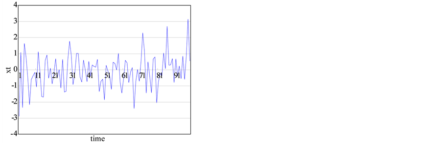
This study tests the time series with the known Hurst exponents as shown in 1) to 4) in below and the series generated from chaotic system and a nonlinear stochastic model as in 5) to 7). Each series with the size of 1000 is generated from the systems and the time series plots are shown in Figure 1.
1) Gaussian white noise; iid (identified independant distribution); H ~ 0.5
 (1)
(1)
where, : normal distribution with mean 0 and standard deviation 1 t: time 2) Fractional Gaussian noise with long range correlation (FGN); H ~ 0.8
 (2)
(2)
where, : Fractional Brownian motion.
3) Autoregressive model (AR(1)) with ρ1 = 0.7
 (3)
(3)
where, : lag-1 autocorrelation coefficient.
 : White noise 4) Fractionally Differenced ARMA (FARIMA); H ~ 0.8; ARIMA (1,0.3.1)
 (4)
(4)
where, : parameter of AR model
 : parameter of MA model
 : back shift operator
 : H–1/2 5) Three torus—quasi-periodic function
 (5)
(5)
where, t; time
 (a)
(a)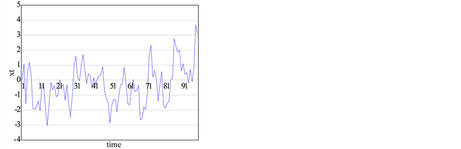 (b)
(b)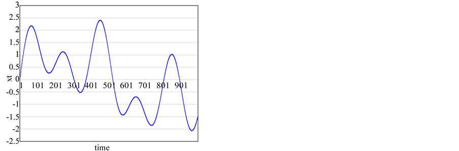 (c)
(c)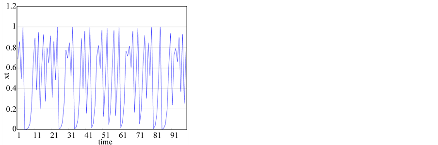 (d)
(d)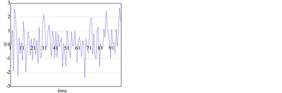 (e)
(e)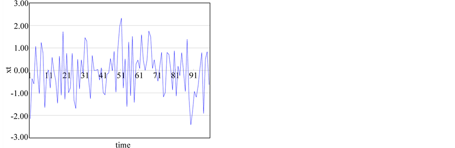 (f)
(f)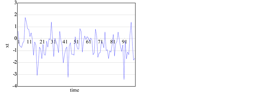 (g)
(g)
Figure 1. The generated time series from chaotic and stochastic systems. (a) white noise; (b) AR(1); (c) Three torus; (d) Logistic map; (e) TAR(2,1); (f) FARIMA; (g) FGN.
6) Logistic map
 (6)
(6)
where, t: time 7) Threshold autoregressive model (TAR(2,1))
 (7)
(7)
where, t: time.
2.2. Methods for the Estimation of Hurst Exponent@NolistTemp#(1) Adjusted Range
[1], examined several sequences of streamflow and observed that for a sequence of n, 1 ≤ n ≤ N, the adjusted range statistic, denoted by R, is defined as
 (8)
(8)
 (9)
(9)
 (10)
(10)
where,  time series,
 : adjusted range statistic
 : mean
 : standard deviation.
(2) Rescaled Range
The rescaled range statistic has been used extensively since its formulation by Mandelbrot. For a time series of n observations,  , the rescaled range statistic, denoted by Q(n), is defined as
 (11)
(11)
 (12)
(12)
where,  time series,
 : size of the entire series
 : size of the partial series
 : the standard deviation of the partial series.
[3], used so many annual time series to estimate the Hurst exponent and obtained the following relations with the calculation of Q(n)
 (13)
(13)
where, : Hurst exponent
 : size of the partial series
 : constant.
Equation (13) can be transformed with the logarithm and Hurst exponent can be estimated from the equation
 (14)
(14)
(3) Modified Rescaled Range
[13], pointed that the regression coefficients can be biased by the autocorrelation when the Hurst exponent is estimated by the regression equation from the known rescaled range. Thus, the rescaled range is a proper method for the time series of the long term memory but it is not for the short term memory. [13], developed the modified rescaled range method like the Equations (15) to (17) and [14,15] applied the method.
 (15)
(15)
 (16)
(16)
 (17)
(17)
where, : weighted sum of autocovariances
 : weighted autocovariance function
 : autocovariance estimator
 : sample variance
 : Truncation lag of the weighted autocovariance function.
Here, we may carefully determine the truncation lag, q of weighted autocovariance function for the application of the modified rescaled range method. If q is so small, the effect of short range could not be considered, while q is so big the long range could be ignored [16]. Thus, the optimal truncation lag, qopt should be estimated. [17], suggested the q = n0.25 and [16] Equation (18). [15], used the modified rescaled range method with q = N/10. However this study will use the Equation (18) [7].
 (18)
(18)
where, : first order autocorrelation coefficient.
(4) 1/f Power Spectral Density Analysis
Power Spectral Density (PSD) has been used in the fields such as physiology, hear rate variability, and the self similarity of brain waves for the estimation of Hurst exponent. Trend in the PSD is proportional to 1/fα and the trend of 1/f is represented by the straight line with the slope of α and the –α can be calculated from the regression of low frequency band. The slope of α and Hurst exponent have the following relationship [6].
 (19)
(19)
where, : 1/f power spectral density
 (20)
(20)
 (21)
(21)
The method of DFA has proven as a useful tool in revealing the extent of long-range correlation in time series. Firstly, the time series to be analyzed (with N samples) is integrated and the integrated time series is divided into boxes of equal length, n. In each box of length n, a least squares line is fit to the data (representing the trend in that box). The y-axis of the straight line segments is denoted, by yn(k). Next, we detrend the integrated time series, y(k), by subtracting the local trend, yn(k), in each box. The root mean square fluctuation of this integrated and detrended time series is calculated by Equations (22) and (23)
 (22)
(22)
 (23)
(23)
This computation is repeated over all time scales (box sizes) to characterize the relationship between F(n). The average fluctuation, as a function of boxes size, Typically, F(n) will increase with size n. A linear relationship on a log-log plot indicates the presence of power law scaling. Under such conditions, the fluctuations can be characterized by a scaling exponent d, the slope of the linear relation of log F(n) vs. logn.
The d has the following relationship and this relationship is represented by Equation (24). Then, The Hurst exponent is estimated by Equations (20) and (21).
 (24)
(24)
(6) Aggregated Variance Time Metho
Firstly, the mean value is obtained with the block of N/m by using Equations (25) and (26) for the time series Xi  (see the Figure 2).
 (25)
(25)
 (26)
(26)
For successive values of m, the sample variance of the aggregated series is plotted by m vs. log-log plot. The result should be a straight line with a slope of β and β has the following relationship:
 (27)
(27)
In practical, the slope is estimated by fitting a least-squares line to the points of the plot.
(7) Maximum Likehood Estimation(MLE)
Here the d is estimated by the S-MLE function of S-Plus [18], and the d is related to the Hurst exponent as follows;
 (28)
(28)
2.3. Applications of the Hurst Exponent Estimation Methods
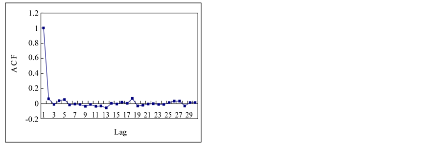
Finally, complete content and organizational editing before formatting. Please take note of the following items when proofreading spelling and grammar: This section is to apply previous mentioned techniques for the estimation of Hurst exponent to the time series in a Section 2.1. Figure 3 shows the autocorrelation functions (ACF) of the time series. If we see the ACFs, the white noise and logistic map show the short term memory and others show the long term memory. Theoretical results for normal independent processes [3], indicated that asymptotically h = 1/2. One interpretation of the Hurst phenomenon has been to associate h = 1/2 with short memory models possessing short-term dependence structure, and h > 1/2 with long memory models possessing long-term dependence [19].
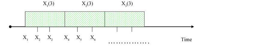
Figure 2. Aggregation of time series.
 (a)
(a)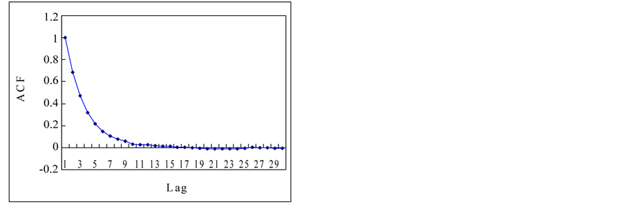 (b)
(b)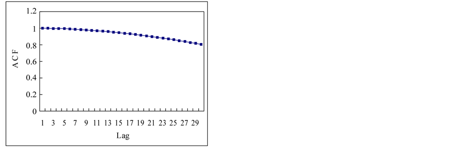 (c)
(c)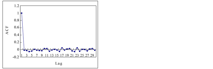 (d)
(d)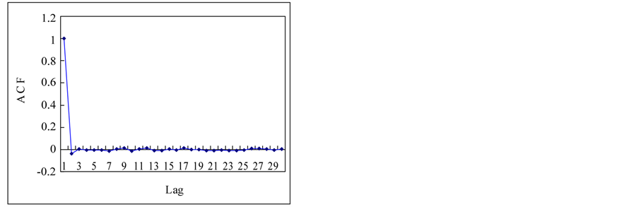 (e)
(e)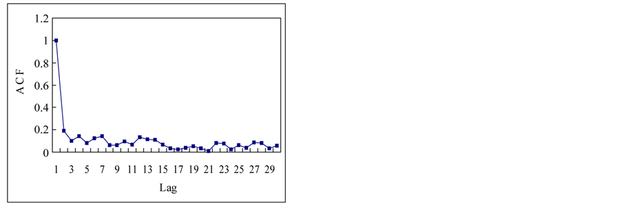 (f)
(f)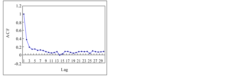 (g)
(g)
Figure 3. Autocorrelation functions of time series from chaotic and stochastic systems. (a) White noise; (b) AR(1); (c) Three torus; (d) Logisitic map; (e) TAR(2,1); (f) FARIMA; (g) FGN.
(1) Rescaled Range and Modified Rescaled Range
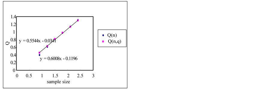
The rescaled range and the modified rescaled range methods are applied to the time series for the error estimation of the methods. Figure 4 shows the comparison of Hurst exponents estimated by the rescaled and modified rescaled range methods. As we can see in Figure 4, the slopes estimated by the rescaled and modified rescaled range methods for the time series of short term memory characteristic are similar. However, the slopes for the time series of long term memory show relatively large differences.
If the sample size is small, the error is small but the error is increased as the sample size is increased as shown in Figure 5. Even though the white noise is a random series, the Hurst exponent is estimated as 0.604 which represents the long term memory by the rescaled range method. However, if we use the modified rescaled range method the exponent is estimated as 0.55 which represents the short term memory (also see Figure 6).
(2) 1/f Power Spectral Density Analysis
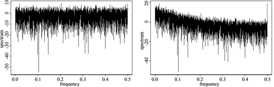
We perform 1/f power spectral density (PSD or periodogram) analysis for the estimation of  and obtain the Hurst exponents by the Equations (20) and (21) for the time series mentioned in Section 2.1. Figure 7 shows the results of PSD analysis for each time series and this method shows relatively reasonable Hurst exponents as we can see in Table1 However, this PSD method may have a problem for the strong persistence system such as the three torus time series which is a quasi-periodic (see Table 1).
(3) Detrended Fluctuation Analysis
This section estimates the Hurst exponents by using DFA method. The Hurst exponent is estimated by the Equations of (20) and (21). Table 2 shows the results of d and Hurst exponents. The DFA method shows the most reasonable Hurst exponent estimates for all-time series as shown in Table2
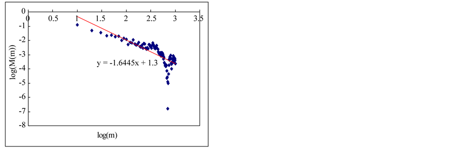
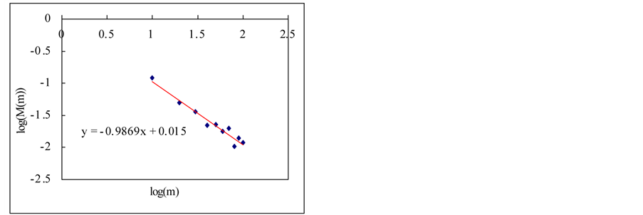
(4) Aggregated Variance Time Method
In this section, we estimate Hurst exponent of time series by means of the aggregated variance time method (AVM). As shown in Figures 8 and 9, the AVM shows the property which the plotted points are scattered for the partial series is over a certain size, the slopes of the straight lines were obtained by the regression, and the Hurst exponents are estimated by Equation (27). However, the exponents are different from the known values. If we estimated the Hurst exponents after removing the scattered points the estimated exponents were similar with the known values (Tables 3 and 4).
Case I: Hurst exponent estimation by the regression with all points;
Case II: Hurst exponent estimation by the regression without the scattered points.
(5) Maximum Likelihood Estimation(MLE)
We estimate the Hurst exponents for the time series by using the statistical package of S-MLE in S-Plus. The results are shown in Table 5 and we can know that the MLE method gives very reasonable values for each time series. Maximum likelihood estimation for FARIMA models can be performed in several ways [20]. We applied here an approximation in the spectral domain of the Gaussian maximum likelihood function, which was first proposed by [21], for short-memory models.
2.4 Results and Discussions
From the analysis of results, the Hurst exponent has estimated appropriately for the long term memory series by the adjusted and rescaled range methods but it was not for the short term memory like a white noise. The modified rescaled range method estimated the Hurst exponent properly for the short term memory series but it was not proper for the long term memory series. The 1/f PSD method estimated the Hurst exponents properly for the series except for the three torus case. The DFA and MLE methods have shown the reasonable results for the short and long term memory series. Especially, the DFA method is more convenient for the application than the MLE. Figure 6 shows the comparison for the Hurst exponent estimation results.
3. Application of DFA for Tree-Ring and SOI Series
We found that the DFA is the most appropriate technique for the Hurst exponent estimation for both the short term memory and long term memory. In this section, we analyze 6 tree-ring series at USA sites and the SOI (Southern Oscillations Index) by means of DFA and the BDS statistic is used for nonlinearity test of the series. Especially, the BDS statistic is used for the nonlinearity of tree ring series tested by [14], who showed the tree ring series has random characteristics. The random characteristic means short term memory and may represent linear stochasticity of the series. Therefore we will examine the memory of tree ring series in the following sections.
 (a)
(a)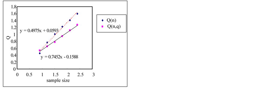 (b)
(b)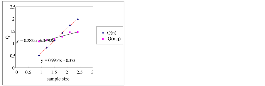 (c)
(c)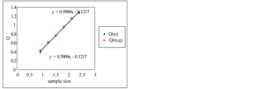 (d)
(d)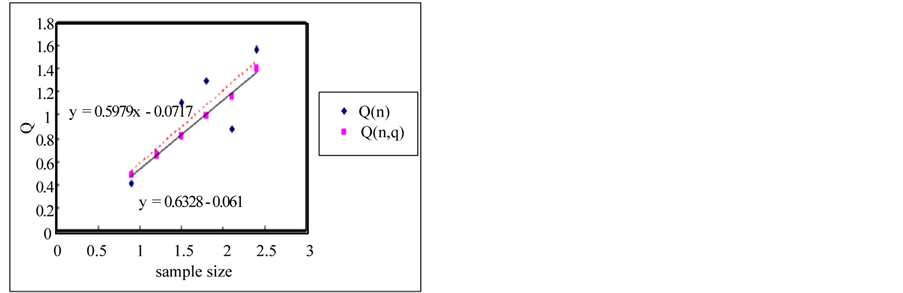 (e)
(e)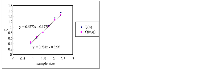 (f)
(f)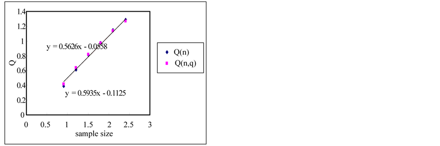 (g)
(g)
Figure 4. Estimation of hurst exponent by rescaled range and modified rescaled range methods. (a) White noise; (b) AR(1); (c) Three torus; (d) Logistic map; (e) FGN; (f) FARIMA; (g) TAR(2,1).
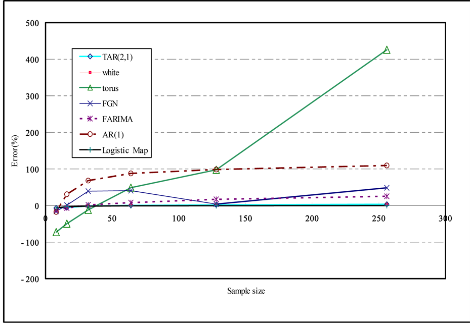
Figure 5. Errors for the rescaled range and modified rescaled range methods.
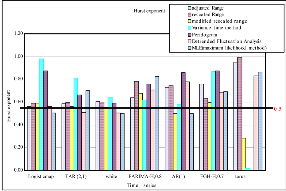
Figure 6. Comparison of the Hurst exponent estimates from various methods.
 (a)
(a)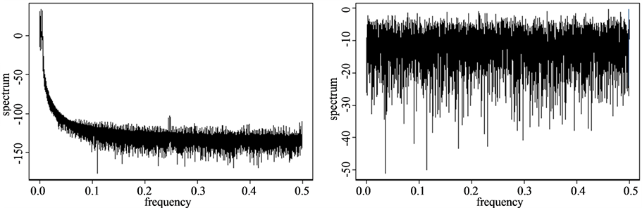 (b)
(b)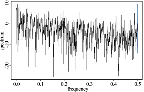 (c)
(c)
Figure 7. 1/f Power spectral density analysis. (a) White noise; (b) AR(1); (c) TAR(2,1); (d) FARIMA; (e) FGN.

Table 1. 1/f spectral slope and hurst exponent.
Table 2. d slope and hurst exponent.
 (a)
(a)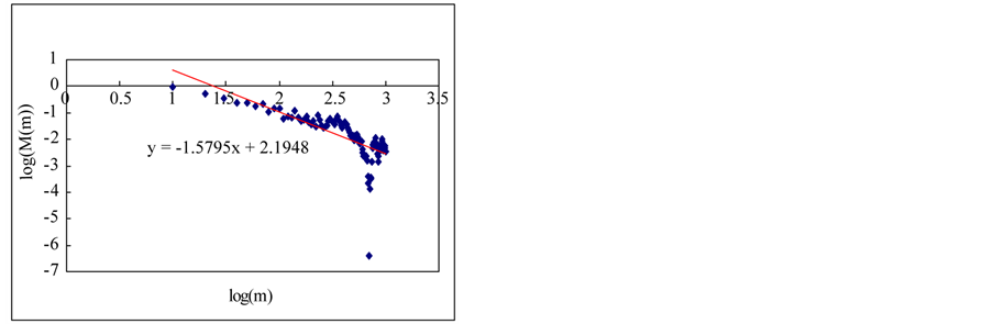 (b)
(b)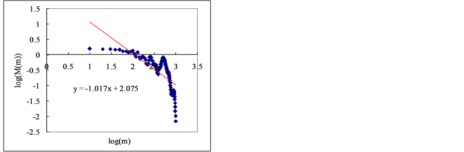 (c)
(c)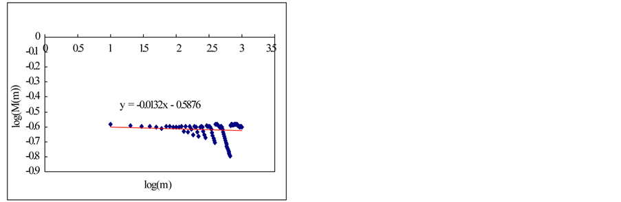 (d)
(d)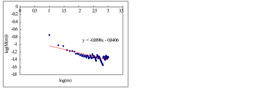 (e)
(e)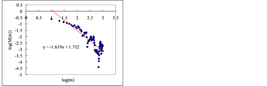 (f)
(f)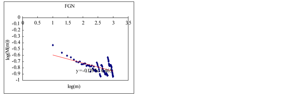 (g)
(g)
Figure 8. Estimation of Hurst exponent by Aggregated Variance Time method (case-I). (a) White noise; (b) AR(1); (c) Three torus; (d) Logistic map; (e) TAR(2,1); (f) FARIMA; (g) FGN.
 (a)
(a)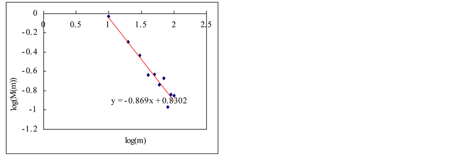 (b)
(b)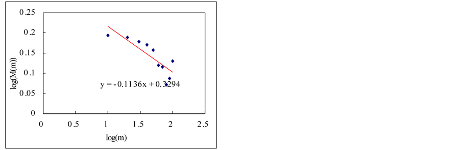 (c)
(c) (d)
(d)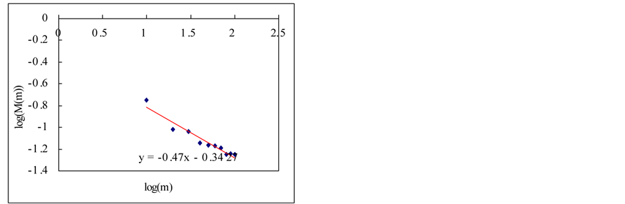 (e)
(e)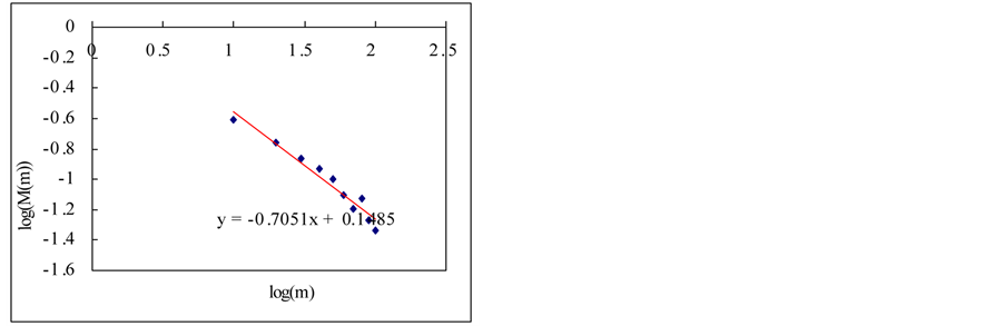 (f)
(f)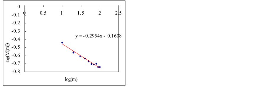 (g)
(g)
Figure 9. Estimation of Hurst exponent by aggregated variance time method (case-II). (a) White noise; (b) AR(1); (c) Three torus; (c) Three torus; (d) Logistic map; (f) FARIMA; (g) FGN.
Table 3. β slope and hurst exponent (case-I).
H = 1 – 2β.
Table 4. β slope and hurst exponent (case-II).
H = 1 – 2β.
Table 5. d slope and hurst exponent.
3.1. Descriptions of Tree-Ring and SOI Series
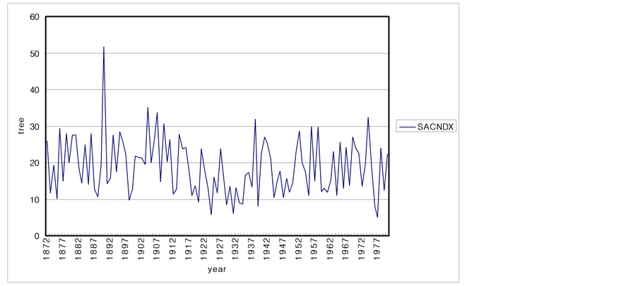
The climatic characteristics of an area are reflected in the growth of the trees. Consequently, the characteristics of tree are studied to determine the long-term climate behavior of a region. In this section, 6 tree ring series from USA are analyzed. The data sets of tree ring series consist of the period of 1892 to 1980 and sites are SACNDX, Spring, Freder, Calam, Hager, Dalton in California and Arizona. Tree-ring data are recorded as local climate properties and annual time scale. Each time series plot is shown in Figure 10.
The SOI is defined as the normalized pressure difference between Tahiti and Darwin. SOI values are calculated using the monthly mean sea level pressure (MSLP) data at papeete, Tahiti (149.6˚W, 17.5˚S) and Darwin, Australia (130.9˚W, 12.4˚S). In this study, we use the monthly SOI data from January of 1951 to December of 1999. Figure 11 shows the time series plot of SOI.
3.2. Hurst’s Memory for Tree-Ring and SOI Data by DFA
Figure 12 shows the comparison of regression plots and results are shown in Table6 Figure 13 shows the comparison of the autocorrelation (ACF) for tree-ring and SOI data. From the results, we found that the SOI series is time series which has a long term memory of H = 0.92. However, contrary to earlier work of [14], all the tree-ring series are not random and some of them show strong persistence from our analysis. A certain tree-ring series shows a long term memory of H = 0.97. Therefore, we can say that the tree ring and SOI series may show long term memory. And if the tree ring series are random as tested in [14], it may have linear stochasticity but the tree ring series which shows long term memory may have its nonlinearity and this could be modeled by the nonlinear stochastic models. Therefore, we would like to examine the nonlinearity of the tree ring and SOI series.
3.3. Nonlinearity for Tree-Ring and SOI Series
The BDS statistic is derived from the correlation integral and has its origins in the recent work on deterministic nonlinear dynamics and chaos theory. The method of delays can be used to embed a scalar time series  into an m-dimensional space as follows
 (29)
(29)
where t is the index lag. The correlation integral at embedding dimension m is given by
 (a)
(a)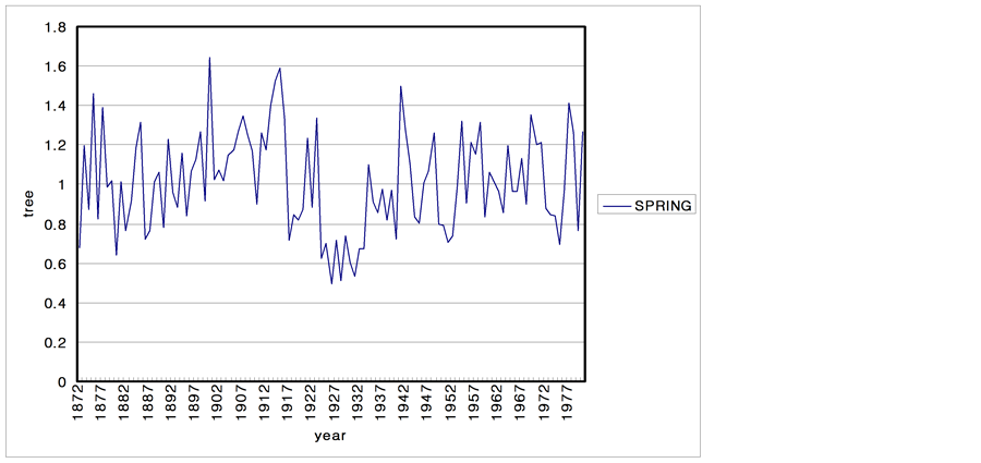 (b)
(b)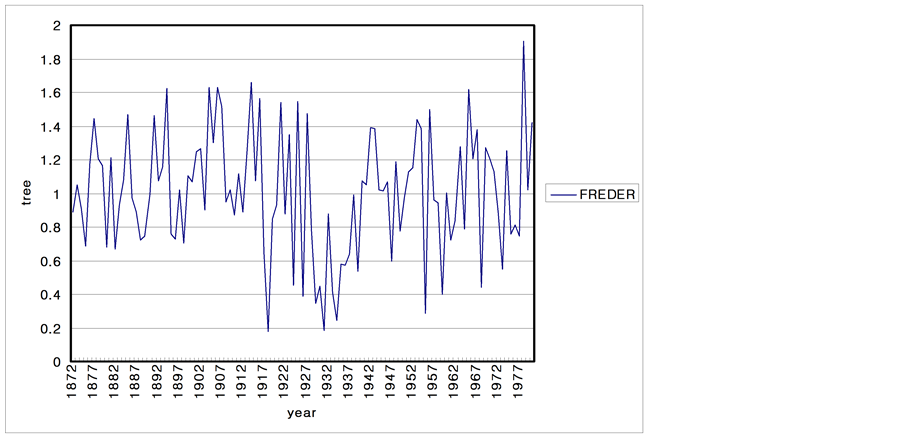 (c)
(c)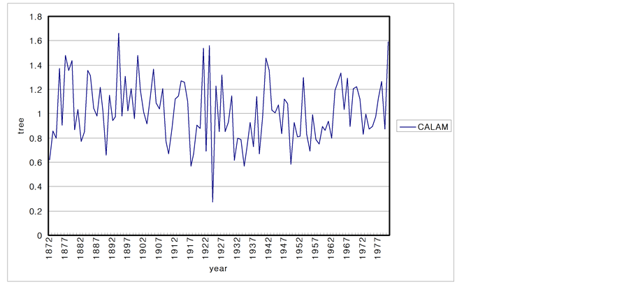 (d)
(d)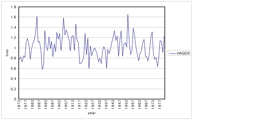 (e)
(e)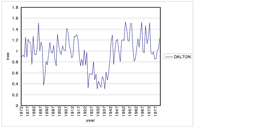 (f)
(f)
Figure 10. Time series plots of the tree-rings. (a) SACNDX; (b) Spring; (c) Freder; (d) Calam; (e) Hager; (f) Dalton.
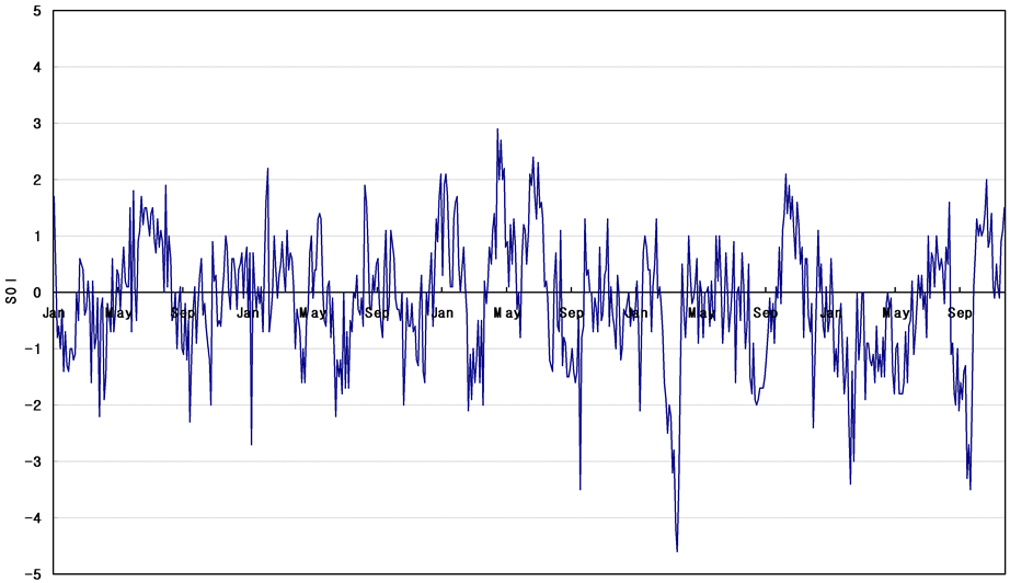
Figure 11. Time series plots of SOI.
monthly
Table 6. Estimations of the Hurst exponent by DFA for the tree rings and SOI series.
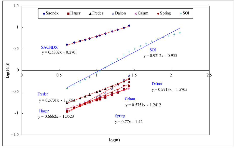
Figure 12. Comparison for regression plots by DFA.
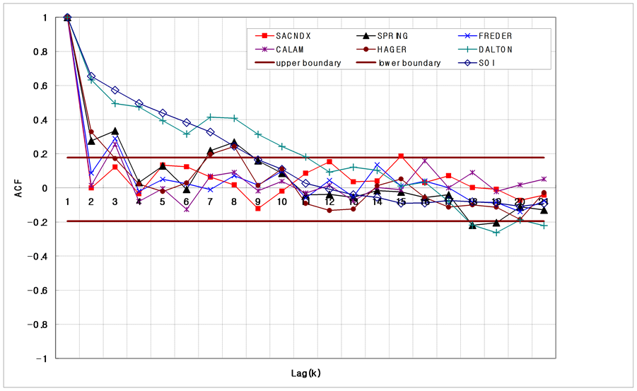
Figure 13. Comparison of the autocorrelation for tree-ring and SOI series.
 (30)
(30)
 where N is the size of the data sets,
  is the number of embedded points in m-dimensional space, and
  denotes the sup-norm.
  measures the fraction of the pairs of points
 ,
,  , whose sup-norm separation is no greater than r. If the limit of
  as
as  exists for each r, we write the fraction of all state vector points that are within r of each other as
 .
.
If the data is generated by a strictly stationary stochastic process which is absolutely regular, then this limit exists. In this case the limit is as follows
 (31)
(31)
When the process is IID, and since , Equation (31) implies that
 . Also
  has asymptotic normal distribution, with zero mean and variance as follows
 (32)
(32)
We can consistently estimate the constants  by
by  and
and  by
by
 (33)
(33)
Under the IID hypothesis, the BDS statistic for m > 1 is defined as
 (34)
(34)
has a limiting standard normal distribution under the null hypothesis of IID as M ® ¥ and obtain its critical values using the standard normal distribution.
Before applying the BDS statistic, the first addressed issue is what region of “r” yields BDS statistic that are well approximated by the asymptotic distribution. As the sample size is increased, the distribution of the BDS statistic becomes more normal. So the minimal number of data must be provided. Next, the region of embedding dimension “m” should be suggested. If the sample size is fixed, we expect the finite sample property to worsen as “m” increases. This study follows the recommendation of [22] for selecting the ranges of m, r, N. Therefore, 500 or more observations are prepared and the embedding dimension m is used in the range of . Then, the value of “r” is selected as the half standard deviations of the data sets. The BDS statistic is a powerful tool for distinguishing random time series from the time series generated by nonlinear systems [22].
We use the BDS statistic for testing randomness of tree-ring and SOI data series and the results are shown in Table7 From the results, the SOI and certain tree-ring are representing their nonlinearities and thus could be modeled by the nonlinear type models [23].
4. Summary and Conclusions
This study has used the seven methods for the estimation of Hurst exponent and compared the results by applying each method to the generated time series form chaos and stochastic systems which have different characteristics. Then, this study discusses the advantages and disadvantages of the techniques and also the limitations of them.
Table 7. The BDS statistics for tree-ring and SOI.
1) The adjusted and rescaled range methods were proper for the long-term memory but the modified rescaled rang method was okay for the short-term memory. These methods have shown that the error was increased as the sample size was increased. Especially the error is increased for the series which the ACF is large.
2) The aggregated variance time method has shown that the plotted points on the proper scale were scattered. And so the Hurst exponent was appropriately estimated when we used the regression after removing the scattered points.
3) The 1/f PSD method has shown that it is a reasonable technique for the Hurst exponent estimation but it was not proper for a very strongly auto correlated series like a three tours system.
4) The DFA and MLE methods have shown that they are the most appropriate techniques for the Hurst exponent estimation for both the short term memory and long term memory.
From these results, we found that the DFA is the most appropriate technique for the Hurst exponent estimation for both the short term memory and long term memory. We analyzed the 6 tree-ring and SOI series for their memory tests by means of DFA and then the BDS statistic has used for nonlinearity test of the series. Our analysis has obtained the following conclusions 5) We found that SOI series is nonlinear time series which has a long term memory of H = 0.92. Contrary to earlier work of [14], all the tree-ring series are not random from our analysis. A certain tree ring series showed a long term memory of H = 0.97 and nonlinear property. Therefore, we can say that the SOI and tree-ring series may show long term memory and nonlinearity.
REFERENCES
- H. Hurst, “Long-Term Storage Capacity of Reservoirs,” Translation of the American Society of Civil Engineer, Vol. 116, 1951, pp. 770-799.
- D. Koutsoyiannis and A. Efstratiadis, “Climate Change Certainty versus Climate Uncertainty and Inferences in Hydrological Studies and Water Resources Management,” 1st General Assembly of the European Geosciences Union, Geophysical Research Abstracts, European Geosciences Union, Austria, Vol. 6, 2004.
- B. Mandelbrot and J. Wallis, “Robustness of the Rescaled Range R/S in the Measurement of Noncyclic Long Run Statistical Dependence,” Water Resources Research, Vol. 5, No. 5, 1969, pp. 967-988. http://dx.doi.org/10.1029/WR005i005p00967
- P. Herman, “Physiological Time Series: Distinguishing Fractal Noises from Motions,” European Journal of Physiology, Vol. 439, No. 4, 1999, pp. 403-415.
- F. Pallikari, “Rescaled Range Analysis of Random Events,” Journal of Scientific Exploration, Vol. 13, No. 1, 1999, pp. 25-40.
- T. Bigger, C. Richard, A. B. Steinman, M. Linda, L. Joseph and J. Richard, “Power Law Behavior of RR-Interval Variability in Healthy Middle-Aged Persons, Patients with Recent Acute Myocardial Infarction, and Patients with Heart Transplants,” Circulation, Vol. 93, No. 12, 1996, pp. 2142-2151. http://dx.doi.org/10.1161/01.CIR.93.12.2142
- M. S. Taqqu and V. Teverovsky, “Estimation for Long Range Dependence: An Empirical Study,” Fractals, Vol. 3, No. 4, 1995 pp. 785-798. http://dx.doi.org/10.1142/S0218348X95000692
- Y. Zhao, “Self-Similarity in High Performance Network Analysis,” University of Missouri-Columbia, Columbia, 1998.
- S. Zafer and T. Sirin, “Traffic Engineering for Multimedia Networks; Data Collection on the Internet, Extensions to Wireless,” NSF industry/University Co-Operative Research Center for Digital Video & Media, 1999.
- M. A. Ausloos, “Statistical Physics in Foreign Exchange Currency and Stock Markets,” Physica A, Vol. 285, No. 1-2, 2000, pp. 48-65. http://dx.doi.org/10.1016/S0378-4371(00)00271-5
- J. W. Kantelhardt, B. E. Koscielny, H. A. Rego, S. Havlin and A. Bunde, “Detecting Long Range Correlations with Detrended Fluctuation Analysis,” Physica A, Vol. 295, No. 3-4, 2001, pp. 441-454. http://dx.doi.org/10.1016/S0378-4371(01)00144-3
- C. M. Kendziorski, “Evaluation Maximum Likelihood Estimation Methods to Determine the Hurst Coefficient,” Physica A, Vol. 273, No. 3-4, 1999, pp. 439-451. http://dx.doi.org/10.1016/S0378-4371(99)00268-X
- A. W. Lo, “Long Term Memory in Stock Market Prices,” Economtrica, Vol. 59, No. 5, 1991, pp. 1279-1313. http://dx.doi.org/10.2307/2938368
- A. R. Rao and D. Bhattacharya, “Hypothesis Testing for Long Term Memory in Hydrologic Series,” Journal of Hydrology, Vol. 216, No. 3-4, 1999, pp. 183-196. http://dx.doi.org/10.1016/S0022-1694(99)00005-0
- A. R. Rao and D. Bhattacharya, “Effect of Short-Term Memory on Hurst Phenomenon,” Journal of Hydrologic Engineering, Vol. 6, No. 2, 2001, pp. 125-131. http://dx.doi.org/10.1061/(ASCE)1084-0699(2001)6:2(125)
- V. Teverovsky, M. S. Taqqu and W. Willinger, “Acritical Look at Lo’s Modified R/S Statistic,” Journal of Statistical Planning and Inference, Vol. 80, No. 1-2, 1998, pp. 211-227.
- P. Philips, “Time Series Regression with a Unit Roof,” Econometrica, Vol. 55, No. 2, 1987, pp. 703-705. http://dx.doi.org/10.2307/1913237
- MathSoft, “S-Plus2000; Guide to Statistical and Mathematical Analysis,” StatSci Dvision, Seattle, 2000.
- J. D. Salas and R. Pielke, “Stochastic Characteristics and Modeling of Hydroclimatic Processes,” In: T. D. Potter and B. Colman, Eds., Handbook of Weather, Climate, and Water, Chapter 32, John Wiley & Sons, New York, 2002, pp. 585-603.
- J. Beran, “Statistics for Long-Memory Processes,” Chapman and Hall, New York, 1994.
- P. Whittle, “Estimation and Information in Stationary Time Series,” Arkiv för Matematik, Vol. 2, No. 5, 1953 pp. 423-434. http://dx.doi.org/10.1007/BF02590998
- H. S. Kim, D. S. Kang and J. H. Kim, “The BDS Statistic and Residual Test,” Stochastic Environmental Research and Risk Assessment, Vol. 17, No. 1-2, 2003, pp. 104-115. http://dx.doi.org/10.1007/s00477-002-0118-0
- J. H. Ahn and H. S. Kim, “Nonlinear Modeling of El Nino/Southern Oscillation Index,” Journal of Hydrologic EngineeringASCE, Vol. 10, No. 1, 2005, pp. 8-15. http://dx.doi.org/10.1061/(ASCE)1084-0699(2005)10:1(8)
NOTES

*Corresponding author.