ABSTRACT

Received October 19, 2013; revised November 19, 2013; accepted November 26, 2013

Ewald summation method, based on Non-Uniform FFTs (ENUF) to compute the electrostatic interactions and forces, is implemented in two different particle simulation schemes to model molecular and soft matter, in classical all-atom Molecular Dynamics and in Dissipative Particle Dynamics for coarse-grained particles. The method combines the traditional Ewald method with a non-uniform fast Fourier transform library (NFFT), making it highly efficient. It scales linearly with the number of particles as, while being both robust and accurate. It conserves both energy and the momentum to float point accuracy. As demonstrated here, it is straight- forward to implement the method in existing computer simulation codes to treat the electrostatic interactions either between point-charges or charge distributions. It should be an attractive alternative to mesh-based Ewald methods.

Keywords:

Ewald Summation Method; Non-Uniform Fast Fourier Transform; Dissipative Particle Dynamics

1. Introduction

Computer modeling and simulation of molecular systems is an established discipline rapidly expanding and widely used from Materials Science to Biological systems. At finite temperatures and normal pressures, molecular compounds are in continuous rapid motion. In liquids and solutions, molecules collide and interact with each other at close distances. They also interact with external fields. In computer simulations of molecular systems, mechanistic ball and spring models are commonly employed to give a simple picture of atoms with specific sizes and masses bonded together with covalent bonds. Molecular equilibrium geometries and interactions are defined by so-called force fields where a somewhat arbitrary division between intramolecular and intermolecular interactions is made, because this partitioning is a simplification of the more detailed and fundamental understanding furnished by a quantum mechanical description.

Intramolecular interactions are normally described by bond stretching, angle bending and torsional angle motion terms. These interactions involve the closest bonded atoms described by two-, three-, and four-body terms, respectively. The bond and angle terms are normally given as harmonic wells while the torsion term is most often expressed as a Fourier sum.

Intermolecular interactions are those between separate molecules but also include all interactions within the same molecule beyond the bonded interactions. Non-bonded interactions are further divided between short- ranged and long-ranged interactions. The short-range interactions mimic the Van der Waals type of forces, while the long-range interactions are electrostatic interactions. The electron distributions around atoms are approxi- mated by fixed point charges, and their interactions are treated by using Coulomb’s law.

The effective range of short-range interactions is limited to a specified cut-off. By assuming a uniform beyond the cut-off, correction terms to the energy can be obtained by integrating over the non-zero part of the inter- actions [1-3]. Thus the fast-decaying short-range interactions can be accurately approximated by truncation at the cut-off distance in most calculations.

Artificially collecting and dividing the diffuse and fluctuating electron densities inside and around molecules on single atomic sites are a crude but conceptually simple and effective approximation, since Coulomb’s law can be invoked. However, this simplification comes at a price since the interactions between point charges stretch over very long distances. Furthermore, these long-range interactions cannot be truncated without introducing simulation artifacts [4-7].

As the system size grows, calculating the electrostatic interactions becomes the major computational bottleneck. Methods based on Ewald summation [8,9] are still considered as the most reliable choice, and a large variety of schemes to compute them in computer simulations have been proposed [10-16]. There is also a multitude of alternative methods for representing electrostatic interactions. Examples are methods based on a cut-off [17-19], tree and multipole based methods [20-25], multigrid methods [26-28], reaction field methods [29-31], the particle mesh method [32,33] and the isotropic sum method [34].

In this paper, we describe an approach to Ewald summation based on the non-uniform fast Fourier transform technique. We use the acronym ENUF-Ewald summation using Non-Uniform fast Fourier transform (NFFT) technique. Our method combines the traditional Ewald summation technique with the NFFT to calculate electrostatic energies and forces in molecular computer simulations. In the paper, we show that ENUF is an easy-to-implement, practical, and efficient method for calculating electrostatic interactions. Energy and momentum are both conserved to float point accuracy. By a suitable choice of parameters, ENUF can be made to behave as traditional Ewald summation but at the same time gives a computational complexity of, where is the number of electrostatic interaction sites in the system. Weighing all these properties together, we believe that ENUF should be an attractive alternative in simulations where the high accuracy of Ewald summation is desired.

In the next section, we summarize the basic methodology to apply Ewald summation to computing the electrostatic energies and forces within periodic boundary conditions. In Section 3, we introduce the Ewald method where the reciprocal space part is calculated based on non-uniform FFTs and discuss the underlying concepts and use of the libraries. We also give general guidelines to implement the method in existing simulation programs. In Section 4, we discuss its implementation in a general purpose atomistic Molecular Dynamics simulation package M.DynaMix giving its scaling characteristics in a standard desktop computer. In Section 5, we demonstrate its implementation in Dissipative Particle Dynamics package. This method is applied to simulating soft charged mesoscopic particles. It is necessary to use charge distributions in order to avoid non-physical aggregation of soft charged particles if point charges are used. This issue is discussed further in Section 5.

2. Electrostatic Interactions

We start by describing a model system of charged particles which captures the most salient features of electrostatic interactions in general MD systems. The electrostatic potential of a system with periodic boundary conditions (PBC) is first stated; we follow with the manipulation of the basic formulas to the form in which they are commonly written; this Section ends with a summary of expressions for both energy and forces.

2.1. Ewald Summation

Consider a cubic simulation box with edge length, containing charged particles, each with a charge, located at. The boundary conditions in a system without cut-off is represented by replicating the simulation box in all directions. The total electrostatic potential energy of the charge-charge interactions is then given by

(1)

where, and denotes the length (2-norm) of the vector. Because of the long-range nature of the electrostatic interactions, includes contributions from all replicas, but exclude self-interactions, which is expressed in the triple sum in Equation (1). The outer sum is taken over all integer vectors

. The symbol on the first summation sign in Equation (1) indicates that

the self-interaction terms should not be included, i.e., when terms are omitted.

The sum in Equation (1) is not an absolutely convergent series, but rather conditionally convergent. As a consequence, the order of summation affects the value of the series. In fact, it was discovered by Riemann that any conditionally convergent series of real terms can be rearranged to yield a series which converges to any prescribed sum [35]. In a sense, this is a situation very similar to the case when a linear equation has an infinite number of solutions because it is under-determined; by adding a set of conditions a unique solution may be defined. For the specific case of Equation (1), a physically relevant summation order has to be prescribed and the boundary conditions of the surrounding media have to be specified.

The lattice sum of Equation (1) can be calculated by a method that was first developed in 1921 by Ewald [8]. He used it to calculate lattice potentials in solids. In the context of Molecular Dynamics, there are several different derivations of the Ewald summation method that are more recent; a small selection is given by [3,9]. In the following discussion we mainly follow the work of de Leeuw et al. [9,36,37].

In [9], de Leeuw et al. developed a technique using convergence factors that transforms the sum of a conditionally convergent series into a series with a well-defined sum. Furthermore, they showed that applying a specific convergence factor is equivalent to a certain summation order. Assuming an overall charge neutral system, , and summing the terms in Equation (1) over all integer vectors in concentric spherical order, they showed that the electrostatic potential energy can be written as

(2)

when the surrounding media of the periodically replicated cell is a uniform dielectric with dielectric constant and distances are calculated with the minimum image convention. When the surrounding media is a conductor, the energy can be written as

(3)

From Equation (3) it is clear that the boundary conditions, vacuum or conductor, have an effect on the energy of the system. Depending on the simulated system and the properties of interest, the choice of boundary conditions can affect the obtained results [38,39].

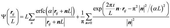
The function is given by

(4)

with the two error functions defined as and. The number used in Equations (2) and (3) is defined as

(5)

where is a free parameter.

Equations (2) and (3) are not in a form that is appropriate for efficient numerical calculations and in the case of Molecular Dynamics simulation we also need expressions for the forces. To arrive at a more suitable form we make the necessary analysis for the electrostatic energy and forces in the following Sections.

2.2. Energies in Ewald Summation

To rearrange and expand Equation (2) we first insert in Equation (4)

(6)

Next we rescale by making the substitution in Equations (5) and (6) to get

(7)

and

(8)

Inserting Equations (7) and (8) into Equation (2) we get

(9)

Note that the summation in Equation (9) is for in the first sum. We make further simplifications by studying the terms on the right hand side of Equation (9) for and.

When we have the following terms

(10)

with the terms independent of n included. The symbol indicates that the terms are excluded from the daggered sum.

When we get

(11)

The factor in Equation (11) comes from changing the summation from to all pairs and, and using the symmetry induced by and.

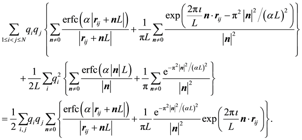
By combining Equations (10) and (11) we identify the real-space term, the reciprocal-space term, the self-interaction term, and the boundary-condition term. The real-space term is given by

(12)

and the reciprocal-space term is

(13)

However, with the symmetries generated by and, we get

(14)

Furthermore, we have

(15)

(16)

and finally

(17)

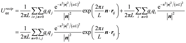
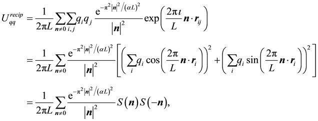
The reciprocal-space part, Equation (14), can be expanded in two different forms. The first form is in terms of the structure factor,

(18)

and is given by

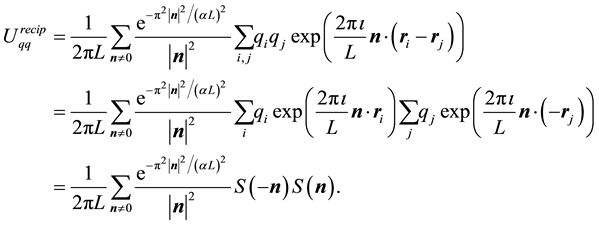(19)

Now for a fixed, the structure factor is just a complex number, and the simple fact that

, gives the real form of Equation (14)

(20)

The first form in Equation (19) is used in our fast approach to calculating the reciprocal-space part. The last form in Equation (20) is the most common point-of-departure when implementing the reciprocal-space part.

2.3. Forces in Ewald Summation

Now that we have calculated the electrostatic energy of the system we can easily compute the electrostatic forces that act on each particle. Splitting the forces in the same way as we have split the energy and using Equation (17) we get the total electrostatic force by finding the negative of the gradient of the electrostatic energy

(21)

The subscript on the operator indicates that we take the partial derivatives with respect to the position of particle and the in Equation (21) comes from the self-interaction term in Equation (15) being independent of. Before we do this calculation we note a couple basic, but helpful, formulas for calculating derivatives

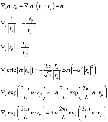(22)

With above formulas, it is straightforward to find the different terms of. The contribution from the real-space term, , becomes

(23)

such that when include all and otherwise only. Equation (20) is convenient to use when calculating the reciprocal-space contribution because it is expressed in terms of charge locations rather than relative distances. Thus the reciprocal-space force is given by

(24)

Finally, the contribution that depends on the boundary condition

(25)

2.4. Formulas for Energy and Forces in Ewald Summation

Consider a periodically replicated system, with the central box consisting of point charges and. Assume that the surrounding media at the boundary of the periodically replicated system is a uniform dielectric with dielectric constant. The cubic box has edge length; each charge is located at, and distances are calculated with the minimum image convention. 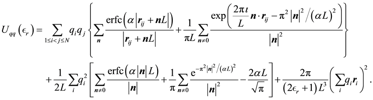After expansion and rearrangements of Equation (2), rescaling and using symmetries induced by and, the total electrostatic energy of the system can be written as

(26)

with the different terms given by

(27)

(28)

(29)

(30)

Note that is a free parameter. The structure factor is defined as

(31)

The total electrostatic force, , on each particle is

(32)

Each of the force terms given by

(33)

(34)

(35)

The positive number, the so called Ewald convergence parameter, is chosen for computational con- venience. Observe that for large values of. By choosing large enough in Equation (27), we can ensure that the only terms that contribute in the real-space sum is when. This may be expressed so that all terms with should be included.

Choose a cut-off in both real-space and reciprocal-space so that the neglected terms in the real-space and reciprocal-space parts are of the same order, or less. The truncation in real-space implies that a sufficient number of terms must be included in the reciprocal-space sums, Equation (28).

Given a required accuracy, is fixed by

(36)

and is determined by

(37)

We have two conditions and four parameters. With a required we may just as well pick a suitable value for and let the above two equations determine and.

With an optimal choice of parameters the computational effort of the Ewald method becomes [36] giving a considerable improvement over the computational complexity implied by the “infinite” reach of the Coulomb interactions.

3. ENUF: A Fast Method for Calculating Electrostatic Interactions

In Section 2 we summarized known results and prepared the ground for the development of a fast method for Ewald summation using the discrete nonuniform fast Fourier transform (NDFT).

3.1. Discrete Fourier Transforms for Non-Equispaced Data

The fast Fourier transform for nonuniform data-points (NFFT) [40] is a generalization of the FFT [41]. Several similar approaches have been proposed; some examples are [42-50] with comparisons in [47,51,52].

The basic idea of NFFT is to combine the standard FFT and linear combinations of a window function that is well localized in both the spatial domain and the frequency domain. A controlled approximation using a cut-off in the frequency domain and a limited number of terms in the spatial domain results in an aliasing error and a truncation error, respectively. The aliasing errors is controlled by the oversampling factor, and the truncation error is controlled by the number of terms, , in the spatial/time approximation. For a number of window functions (Gaussian, B-spline, Sinc-power, Kaiser-Bessel), it has been shown that for a fixed over- sampling factor, , the error decays exponentially with [53].

3.1.1. Problem Definition

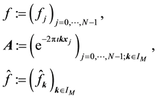
We wish to calculate the discrete Fourier transform for nonequispaced data. The problem can be stated as follows. For a finite number of given Fourier coefficients with we want to evaluate the

trigonometric polynomial at each of the given nonequispaced points

. In the literature, points are often called knots. We use the two terms synonymously.

Obviously, the details of an NDFT depend on the definitions of a sampling set for knots, , and an index space. More in-depth discussions and further details can be found in [53,54]. The presentation that follows is mainly drawn from these sources.

3.1.2. Underlying Concepts

Consider a d-dimensional domain in which the set of nonequispaced knots, or data points, are located. Let

(38)

and the set of data points. For the application we have in mind is usually 2 or 3. Let be a function space of trigonometric polynomials with degree in dimension; the function space can be defined as

(39)

The dimension of this function space is. The frequencies with the index set are such that

(40)

3.1.3. Matrix-Vector Formulation

With these preliminary definitions we carry on with the problem of calculating the discrete Fourier transform for

nonequispaced data. For a finite number of given Fourier coefficients with we want to evaluate the trigonometric polynomial at each of the given nonequispaced

knots in, where the product is the usual scalar product of the two vectors and as. Consequently, for each, we evaluate. This may be reformulated in matrix-vector notation by setting

(41)

and writing.

3.1.4. Related Matrix-Vector Products

A number of related NDFT matrix-vector products can also be defined. To write them down we let be the complex conjugate of the elements of the matrix and the transposed complex conjugate of the matrix. Using these conventions we can name and summarize the related NDFT matrix-vector products and their component representation as

(42)

(43)

(44)

(45)

3.1.5. NDFT, FFT and NFFT

From the different NDFT products written in matrix-vector form, as in Equations (42)-(45), it is clear that it takes arithmetic operations to transform between the Fourier-samples and the Fourier-coefficients.

This is simply because the matrix is, with.

However, for the special case of and equispaced knots, the Fourier-samples can be calculated from the Fourier-coefficients by the fast Fourier transform (FFT) with arithmetic operations.

The fast Fourier transform for nonequispaced knots (NFFT) is a generalization of the FFT. The essential idea is that of combining a window function with the standard FFT. The window function is a well localized function in both the space domain and frequency domain. Several different window functions and similar approaches have been proposed. The resulting algorithms are approximate and some of them have been shown to have a computational complexity of, where is the desired accuracy [53].

3.2. Fast Ewald Summation

Using optimal parameters in the Ewald summation method implies that the time to calculate the real-space part and the reciprocal-space part are approximately equal. As the number of particles in the system grows we would like to combine the calculation of the short-range part of the potential with the real-space part. This implies that we need to choose a real-space cut-off about the same size as the short-range cut-off. With this nonoptimal choice, the reciprocal-space parts of the Ewald summation method become the most time-consuming to calculate [55].

To show how a fast Ewald summation approach may be obtained from the regular Ewald method, described in Section 2, we focus on the reciprocal-space parts. In Section 3.1, we gave the details of the discrete Fourier transform (DFT) for data that is nonuniformly spaced (NDFT). Based on these definitions we get a number of useful algorithmic primitives. First we reformulate the reciprocal-space part of the regular Ewald method in terms of the NDFT primitives. Then we show how the fast Fourier transform for nonequispaced (NFFT) can be applied, yielding an Ewald method based on the nonuniform fast Fourier transform.

3.2.1. Reciprocal Space Terms as DFT

We apply the generalized DFT, described in Section 3.1, to the calculation of the reciprocal-space energy and forces. This allows us to formulate the standard Ewald method for calculating the reciprocal energy and forces in terms of the NDFT primitives.

3.2.2. Reciprocal Energy

In the case of the electrostatic energy we have from Equation (28)

(46)

with the structure factor defined as

(47)

By comparing the definition of the transposed NDFT in Equation (45) and the structure factor in Equation (47) we note that they have the same structure; after a renumbering of the location indexes, the summation limits are also the same. In fact, by setting the normalized locations, , and the samples, , we see by inspection that Equation (47) is a 3D instance of Equation (45) with. Furthermore, assuming that the MD simulation box is centered around the origin, the normalized locations can be assumed to be in the domain as defined in Equation (38).

Consequently, we can use the NDFT approach to calculate each of the components of the structure factor. From a computational point of view this means that we can also expect to utilize an NFFT based algorithm to calculate the components of the structure factor, rather than the straightforward summation normally used in the Ewald method.

Recasting Equation (46) in terms of Fourier-components

(48)

Calculating the energy, , using Equation (48) means that we

1) calculate all using the transposed NDFT,

2) scale each with a factor given by Equation (48),

3) sum all the scaled components.

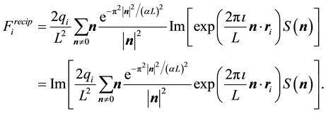
3.2.3. Reciprocal Forces

We calculate the contribution from the reciprocal-space forces using a similar approach as for the energy. In the formula below, , and, denote the real and imaginary part of the arguments, respectively. From Equation (24) we have that

(49)

Now, the structure factor is just a complex number so the expression in the brackets in Equation (49) can be written as the imaginary part of a product

(50)

Inserting Equation (50) this into Equation (49) gives

(51)

Note that Equation (51) is a vector equation. Furthermore, each of the three components has the same structure as the conjugated NDFT of Equation (44). By setting the normalized locations, , and the samples,

(52)

we see, again, by inspection that each component of Equation (51) is a 3D instance of Equation (44). Assuming that is in the index set of Equation (40), , and setting, we can formulate directly in Fourier-terms

(53)

Calculating the reciprocal-space force on particle, using Equation (53), means that we

1) start with the structure factor components, , already obtained when we calulated,

2) scale each using Equation (52),

3) giving a new set of Fourier-coefficients that are transformed back to real-space, via Equation (53), using the conjugated NDFT, and finally

4) with Equation (53), taking the imaginary part of coefficient and scaling it with gives the reciprocal force on particle.

Thus we can use the NDFT approach to calculate each of the components of the reciprocal forces. Again, from a computational point of view this means we can expect to utilize an NFFT based algorithm to find the respective components.

3.2.4. Combining the Ewald Method and NFFT

The reformulation of and as in Equations (48) and (53) shows the central role of the transposed and conjugated NDFT in calculating the reciprocal-space energy and forces. Starting with the location of the charged particles, the structure factor is calculated via a transposed NDFT. In the language of Ewald summation, we transform from real-space to reciprocal-space. Scaling the absolute value of the Fourier- components and summing gives. To find we go back from the reciprocal-space to the real-space by first calculating the Fourier-components of the forces and then performing a conjugated NDFT.

An implementation of Ewald summation uses cut-offs, in reciprocal-space, , and real-space,; with large enough and with a required accuracy, , truncate the sums Equation (27) and Equation (28) at the respective cut-offs so that the last term added, in each of the sums. When is fixed by

(54)

Then is determined by

(55)

We have recast and in terms of Fourier-components and set, where is the

oversampling factor. This gives. In general the computational complexity of the NFFT method

is, where is the desired accuracy in the approximation used within NFFT [53].

Using Equation (54) and the above defintion of, we see that the complexity becomes. Note that is a function of, for a fixed oversampling factor. With a controlled approximation of the structure factor via the use of nonuniform fast Fourier transform, the original computational complexity of becomes.

At this stage, the path to a fast Ewald method should now be clear. By specifying an accuracy, we replace the transposed and conjugated NDFT with the corresponding operations using the NFFT algorithm. Thus Equations (48) and (53) become a concise procedure to calculate approximations of and. Most of the mathematical details can be kept separate and hidden in a set of library routines and the remaining formulas pertain to the physics of the problem. Furthermore, with a library implementation based on a state-of-the-art FFT-library, we have good reason to expect it to be efficient.

3.2.5. Implementation and Results

In a first implementation [56,57], we used the libraries FFTW [58] and NFFT [54]. Details of the accuracy and scaling properties can be found in reference papers.

Basing the implementation on libraries has a number of advantages. It makes the implementation task easier and introduces a convenient division of labor in the program code: the mathematical aspects are mainly concentrated to the libraries while the physical aspects of the problem remain. Also, since the code becomes quite compact without becoming convoluted, it becomes easier to check, understand, and explain. Improvements and optimizations of the libraries can be easily included in the program, usually by just relinking the program. For example, the customization of the window function used in the NFFT algorithm---Gaussian functions, dilated cardinal B-splines, Sinc functions, or Kaiser-Bessel functions---is currently achieved by recompiling the NFFT library and relinking the application. Due to the comparatively small size of the NFFT library this is very quick. Furthermore, improvements in either theory or implementation of the used libraries will be easily accessible.

In summary, we claim that the ENUF method is

・ efficient and concise, and

・ has a clear separation of concerns between mathematical and physical details.

In a sense it can be said that we get the best of two worlds: a concise and efficient algorithm. The separation of mathematical concerns is a bonus that has the potential to simplify implementation and further developments due to the fact that they may occur independently of each-other.

4. ENUF Implemented in M.DynaMix

M.DynaMix is a highly modular general purpose parallel Molecular Dynamics code for simulations of arbitrary mixtures of either rigid or flexible molecules. It was released by Lyubartsev and Laaksonen in late 90’s [59]. Most common force fields can be used in simulations with a variety of periodic boundary conditions (cubic, rectangular, hexagonal or a truncated octahedron). Quantum corrections to the atomic motion can be done using the Path Integral Molecular Dynamics approach. M.DynaMix has been used in applications from materials design to biological processes.

M.DynaMix deals with particle system interacting by a force field consisting of Lennard-Jones, electrostatic, covalent bonds, angles and torsion angles potentials as well as of some optional terms, in a periodic rectangular, hexagonal or truncated octahedron cell. Rigid bonds are constrained by the SHAKE algorithm [60]. In case of flexible molecular models the double time step algorithm is used [61]. Algorithms for NVE, NVT and NPT statistical ensembles are implemented, as well as Ewald sum approach for treatment of the electrostatic interactions. An option to calculate free energy by the expanded ensemble method with Wang-Landau optimization of the balancing factor is included in later versions. For its features and capabilities, M.DynaMix is diffused in a large modeling and simulation community. Written in FORTRAN 77, it can be run on a wide variety of hardware architectures both in sequential and parallel execution. The entire program source code consists of a number of FORTRAN files (modules), made of blocks of subroutines, performing different tasks or groups of tasks.

4.1. Framework Overview

The situation outlined for M.DynaMix is very common in the field of computational science: a package created in late 90’s that is still at work in spite of new innovations in computing platforms. In a situation like this, each upgrade requires a trade-off between the need to preserve the existing structure and the wish to obtain as much efficiency as possible.

To take the best advantage from latest programming techniques and tools, we decide to use C language to create some of the new code segments. On one hand, modules in FORTRAN and C can easily coexist in the same code, just taking account of a few mild guidelines [62]; on the other hand, C language provides several enhancements related to intrinsic features (dynamic memory allocation and direct pointers reference) and possibility to set up complex data structures; furthermore, it allows a more plain access to a large amount of external routine libraries written in C. From a general point of view, M.DynaMix code has been projected with a good modularity degree and has been possible to make the most part of upgrades just switching a block (subroutine) with a new one.

4.2. Input Parameters

To use ENUF method for treating long range interactions, M.DynaMix user needs to set the proper key string in the input file [63]; parameters to specify are the Ewald convergence factor and the number of points for FFT grid in, and direction; starting from them, the program automatically sets proper values for over-sampling factor and approximation parameter.

4.3. Implementation

Ewald-like methods for computing electrostatic energies typically replace part of the summation in real space with an equivalent summation in Fourier space; among M.DynaMix modules, there is one devoted to this reciprocal space duty. In the starting setup, this module was present in M.DynaMix in a version related to the full Ewald algorithm; ENUF implementation involved the creation of a second instance of this module.

A scheme of the ENUF module as implemented in M.DynaMix is presented in Table 1; the module in this case is a group of files, part of them written in FORTRAN and part in C; each file contains routines related to the algorithm steps. The table displays for each step the programming language used to write corresponding file; Some files make calls to external libraries, typically used to perform non uniform Fourier transform and its inverse.

4.3.1. Coordinate Scaling and Adjoint Transform

In the first step of the algorithm, particle coordinates are rescaled respect to the simulation box, in order to obtain the proper set of nonequispaced knots as required in Equation (38). Knots are stored in the unidimensional FORTRAN array, in consecutive way, saving coordinates in reverse component order for each knot. Particle charges are located in unidimensional array.

At the next step, a C routine performs the 3-dim adjoint transform of charges located at knots. C routine access to 1-dim FORTRAN vectors and as three dimensional arrays; the reverse component order adopted in vector filling is related to this and depends on the different way to arrange multi- dimensional arrays in memory: by columns for FORTRAN, by rows for C. Transformed data are stored in the complex array.

4.3.2. Energy, Regular Transform and Forces

In this stage, energy is evaluated by a sum, according to formula (48). Then, the transformed array is rescaled using Equation (51); starting from, three complex rescaled arrays are created, , and,

one for each direction in the reciprocal space. A C routine back transform complex data set, and

related to the same set of knots. In this step, three independent back transformations are performed, producing complex arrays, and. Forces contributions for each particle are obtained according to Equation (53); components in, and directions are evaluated using the imaginary part of arrays, and.

4.4. External Libraries

To perform Fourier transform on nonequispaced data, our current implementation make use of an external existing function library. Among the available resources, we select the library NFFT [54]. NFFT is a widely diffused C subroutine library for computing nonequispaced discrete Fourier transform in one or more dimensions, of arbitrary input size and of complex data; it is based on FFTW [58].

4.5. Validation

In the original version of M.DynaMix the working method for the treatment of long range interactions is the full direct Ewald summation. Using a cross-check approach, namely comparing ENUF method to the stable one, it has been possible to debug every step of the algorithm implementation and check its correctness in deep way.

After the implementation, the same cross-check mechanism has been used to investigate ENUF precision and efficiency. Figure 1 displays the execution time spent for long range interactions evaluation respect to the number of particles N, when full Ewald and ENUF are used. In the simulation, of iterations, the system is composed by 50 ions and 50 ions in water solution in a cubic cell. The number of water molecules is increased from to in seven discrete steps, keeping constant the density to 1.02. The simulation run on a Intel Xeon workstation, 1.86 GHz, with ram 8 Gb.

The full Ewald method has been taken as reference; for each system size, ENUF parameters have been tuned to obtain the same Ewald precision, evaluated in terms of the electrostatics energy contribution, tolerating a maximum divergence of 2%.

The plot shows that execution time for long range interactions that represents the efficiency bottleneck in the original M.DynaMix version, has been drastically reduced saving the same numerical precision. The plot also shows the different trend for execution time vs in the two methods; the point set for the full Ewald scheme

is well fitted using the well-known theoretical behavior; data points related to ENUF correspond quite well to the expected.

5. Implementation of ENUF Method in Dissipative Particle Dynamics Scheme

The Dissipative Particle Dynamics (DPD) simulation method, originally proposed by Hoogerbrugge and Koelman, is a particle-based simulation method to simulate hydrodynamic phenomena at mesoscopic level [64, 65,66]. In DPD model, several atoms or molecules are grouped together to form coarse-grained particles. The interactions between any pair of DPD particles and are normally composed of three pairwise additive forces: the conservative force, the dissipative force, and the random force

(56)

with

(57)

(58)

(59)

where, , , and. The parameters, , and determine the strength of the conservative, dissipative, and random forces, respectively. is a randomly fluctuating variable, with zero mean and unit variance.

The pairwise conservative force is written in terms of a weight function, where is usually chosen for and for such that the conservative force is soft and repulsive. The unit of length is related to the volume of DPD particles. Two weight functions and for dissipative and random forces, respectively, are coupled together through the fluctuation- dissipation theorem

(60)

to form a thermostat and generate naturally the canonical distribution (constant number of particles, N, volume, V, and temperature, T) [67]. In most applications, the weight function adopts a simple form as [68]

(61)

In the original DPD model, one critical advantage is the soft repulsive nature of conservative potential, which enables us to integrate the equations of motion with large time step. However, such advantage restricts the direct incorporation of electrostatic interactions in DPD model. The main problem is that dissipative particles carrying opposite point charges tend to collapse onto each other, forming artificial ionic clusters due to the stronger electrostatic interactions than soft repulsive conservative interactions.

In order to avoid such unphysical phenomena, point charges at the center of dissipative particles are usually replaced by charge density distributions meshed around particles to remove the divergency of electrostatic interactions at [69,70]. In our implementation [71,72], a Slater-type charge density distribution is considered with the form of

(62)

in which is the decay length. The integration of Equation (62) over the whole space gives the total charge.

The electrostatic potential generated by Slater-type charge distribution can be obtained by solving Poisson’s equation

(63)

in which the variables and are the permittivity of vacuum space and the dielectric constant of water at room temperature, respectively. In spherical coordinates, the Poisson’s equation becomes

(64)

By solving Poisson’s equation, the electrostatic potential field can be analytically expressed by

(65)

The electrostatic energy between two interacting charge density distributions and is the product of the charge density distribution and the electrostatic potential generated by charge distribution at position

(66)

The electrostatic force on charge distribution is the negative of the derivative of the potential energy respect to its position

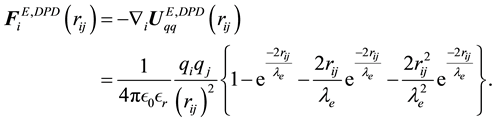(67)

By defining parameter as the reduced center-to-center distance between two charge distributions and dimensionless parameter, respectively, the reduced electrostatic energy and force between two Slater-type charge distributions are given by

(68)

(69)

Comparing to the electrostatic energy and force between point charges in atomistic simulations in previous section, we can find that the electrostatic energy and force between two Slater-type charge distributions in DPD simulations are scaled with corresponding correction factors as

(70)

(71)

The similarities between electrostatic energy and force between point charges and counterparts between charge density distributions imply that once we get electrostatic energy and force between point charges, from which the electrostatic energy and force between Slater-type charge density distributions in DPD simulations can be directly rescaled with corresponding correction factors.

For the electrostatic energy and force between point charges, we know that both of them do diverge when the relative distance between point charges is close to 0. While for the electrostatic energy and force between charge density distributions, in the limit of, the reduced electrostatic energy and force between charge density distributions are, respectively, described by

(72)

(73)

It is clear that the adoption of Slater-type charge distribution in DPD simulations removes the divergence of electrostatic interactions at, which means that both electrostatic energy and force between charge distributions are characterized with finite quantities.

By matching the maximum electrostatic energy between charge distributions at with Groot’s previous work [69] gives. In our detailed implementations, we adopted a particular coarse-graining scheme [73] with and, in which the former parameter means water molecules being coarse-grained into one DPD particle and the latter means there are DPD particles in the volume of. With this particular scheme, the length unit is given as. From the relation of, we can get, which is consistent with the electrostatic smearing radii used in González-Melchor’s work [70].

Figure 2 shows the representation of reduced electrostatic energy and force with respect to the relative distance between Slater-type charge distributions. For a better comparison, we also include the typical soft conservative potential and force between dissipative particles, as well as the standard Coulombic potential and force between point charges, both of which do diverge at. In short range length scale, both the electrostatic energy and force are characterized with finite quantities, which attribute to the adoption of Slater-type charge distributions instead of point charges. In long range length scale, both the electrostatic energy and force are consistent with counterparts between point charges, which implys that the ENUF-DPD method can capture essential characteristics of electrostatic interactions at mesoscopic level.

Combining electrostatic force and soft repulsive conservative force gives the total conservative force on particles in DPD simulations. The total conservative force, together with dissipative force and random force, as well as the intramolecular bonding force for polymers and surfactants, act on dissipative particles and evolve the whole simulated system toward equilibrium conditions before taking statistical analysis.

As the number of charged DPD particles in the simulated system grows, the calculation of the reciprocal space electrostatic interactions will become the most time-consuming part. Using suitable parameters in

ENUF-DPD method assures that the time to calculate the real space summations is approximately the same as the time to calculate the reciprocal space summations, thereby reducing the total computational time. Herein we try to explore the ENUF-DPD related parameters and get a set of suitable parameters for further applications.

As addressed in Section 3.2, the implementation of ENUF-DPD method uses the Ewald convergence parameter, required accuracy, and two cut-offs (for real space and for reciprocal space summations). These parameters are correlated with each other through two conditions shown in Equations (54) and (55). With required accuracy parameter, it is more convenient to pick a suitable value for. Then one can determine and directly from Equations (54). However, due to the fact that should be integer and should be a suitable value for the cell-link list update scheme in DPD simulations, we adopt another procedure to get suitable parameters.

During the calculation of real space summation and self-interaction parts of electrostatic energy and force between point charges, we can directly multiply corresponding correction factors to get the electrostatic energy and force between slater-type charge density distributions. However, it is not accessible for the calculation of reciprocal space summation since we cannot rescale the NFFT transformation results. But if we choose suitable real space cutoff, beyond which two correction factors and converge to unit, one can directly adopt NFFT transformation result without any corrections. We find that electrostatic energy and force between charge density distributions are consistent with counterparts between point charges when the relative distance between two distributions is larger than. Hence in our simulations, is taken as the cutoff for real space summations of electrostatic interactions.

By evaluating the Madelung constant of a face-centered cubic (FCC) lattice, we adopt the Ewald convergence parameter with the value of, which can generate accurate Madelung constant for FCC lattice structure and keep considerable accuracy. Then we perform coarse-grained simulations on bulk electrolyte system to explore suitable values for, and approximation parameter in NFFT. It is specified that approximation parameter and cutoff for reciprocal space summations can generate consistent electrostatic energy and force in comparison with those obtained from traditional Ewald summation method with reference parameters. Larger values can further increase the accuracy of electrostatic interactions in ENUF-DPD method, but also the total computational time in treating electrostatic interactions increases. By compromising the accuracy and computational speed in the ENUF-DPD method, we adopt and in following simulations.

With the set of explored optimized parameters, we address the computational complexity of ENUF-DPD method in treating electrostatic interactions. The computational complexity of ENUF-DPD method is appro- ximately described as, which shows remarkably better computational efficiency than the tradi- tional Ewald summation method with acceptable accuracy in treating long-range electrostatic interactions between charged particles at mesoscopic level.

The ENUF-DPD method is then validated by investigating the influence of charge fraction of polyelectrolyte on corresponding conformational properties [71]. With the increase of charge fraction on polyelectrolyte, both the intramolecular correlations between charged beads on polyelectrolyte chain and the intermolecular correla- tions between charged beads on polyelectrolyte and counterions are enhanced. The conformation transition of polyelectrolyte chain from collapsed state to fully extended conformation can be visualized from simulations. Meanwhile, the dependence of the conformations of fully ionized polyelectrolyte on charge valency and concentration of added salts are also studied in details. Counterions with larger valency show stronger conden- sations on polyelectrolyte chains. Such counterions can induce polyelectrolyte chains from extended confor- mation to compact state, and then to swollen conformation with the increase of counterion concentrations.

With the ENUF-DPD method, we further investigate the specific binding structures of dendrimers on amphiphilic bilayer membranes [74]. We construct mutually consistent coarse-grained models for dendrimers and lipid molecules, which can properly describe the conformation of charged dendrimers and the surface tension of amphiphilic membranes, respectively. Systematic simulations are performed and simulation results reveal that the permeability of dendrimers across membranes is enhanced upon increasing dendrimer sizes. The negative curvature of amphiphilic membrane formed in dendrimer-membrane complexes is related to dendrimer concentration. Higher dendrimer concentration together with the synergistic effect between charged dendrimers can also enhance the permeability of dendrimers across amphiphilic membranes.

With these two typical and representative applications, we can see that the newly implemented ENUF-DPD method can capture the essential characteristics of electrostatic interactions at mesoscopic level. This method has all capabilities of ordinary DPD method, but includes applications where electrostatic interactions are essential but previously inaccessible, hence can be used to study charged complex systems at mesoscopic level.

6. Summary and Conclusions

Treatment of electrostatic interactions based on Ewald summation techniques is reviewed. While Ewald- summation is still considered as the most accurate scheme to compute the long-ranged interactions, it is also the part slowing down simulations. The scaling for large systems makes the computations very time-consuming. In particular, the reciprocal part of Ewald becomes a bottle-neck. As an attractive alternative approach to mesh- based schemes which show a linear scaling, we introduce an Ewald method based on non-uniform fast Fourier transforms (ENUF) giving examples of two implementations in already existing software packages, for ato- mistic Molecular Dynamics and Dissipative Particle Dynamics. We demonstrate that the implementation be- comes straight-forward as we rely on NFFT library. We discuss the optimization of convergence parameters and window functions.

The ENUF method scales linearly as and conserves both the energy and momentum to float point accuracy making it a very robust and accurate method.

Acknowledgements

Y.-L. W. and A. L. acknowledge the KA Wallenberg Foundation for financial support. F. M. acknowledges the Wenner-Gren and the Carl Tryggers Foundations for funding for Visiting Professorship. Y.-L. W. and A. L. thank the Kavli Institute for Theoretical Physics China (KITPC) and Chinese Academy of Sciences (CAS) for support and scientific environment during their stay. This work is supported by SERC the Swedish e-Science Center and Swedish Science Council. Parts of the computations were performed on resources provided by the Swedish National Infrastructure for Computing (SNIC) at PDC, HPC2N, and NSC.

References

- 1. M. P. Allen and D. J. Tildesley, “Computer Simulation of Liquids,” Oxford University Press, New York, 1989.
- 2. J. M. Haile, “Molecular Dynamics Simulation: Elementary Methods,” John Wiley & Sons, New York, 1992.
- 3. D. Frenkel and B. Smit, “Understanding Molecular Simulation: From Algorithms to Applications,” Academic Press, Inc., Orlando, 1996.
- 4. D. M. York, T. A. Darden and L. G. Pedersen, “The Effect of Long-Range Electrostatic Interactions in Simulations of Macromolecular Crystals: A Comparison of the Ewald and Truncated List Methods,” Journal of Chemical Physics, Vol. 99, No. 10, 1993, p. 8345. http://dx.doi.org/10.1063/1.465608
- 5. M. Bergdorf, C. Peter and P. H. Hünenberger, “Influence of Cut-off Truncation and Artificial Periodicity of Electrostatic Interactions in Molecular Simulations of Solvated Ions: A Continuum Electrostatics Study,” Journal of Chemical Physics, Vol. 119, No. 17, 2003, p. 9129.
http://dx.doi.org/10.1063/1.1614202 - 6. C. Anézo, A. H. de Vries, H. D. Holtje, D. P. Tieleman and S. J. Marrink, “Methodological Issues in Lipid Bilayer Simulations,” Journal of Physical Chemistry B, Vol. 107, No. 35, 2003, pp. 9424-9433. http://dx.doi.org/10.1021/jp0348981
- 7. M. Patra, M. Karttunen, M. T. Hyvonen, E. Falck, P. Lindqvist and I. Vattulainen, “Molecular Dynamics Simulations of Lipid Bilayers: Major Artifacts Due to Truncating Electrostatic Interactions,” Biophysical Journal, Vol. 84, No. 6, 2003, pp. 36363645. http://dx.doi.org/10.1016/S0006-3495(03)75094-2
- 8. P. P. Ewald, “Die Berechnung Optischer und Elektrostatischer Gitterpotentiale,” Annalen der Physik, Vol. 369, No. 3, 1921, pp. 253-287. http://dx.doi.org/10.1002/andp.19213690304
- 9. S. W. de Leeuw, J. W. Perram and E. R. Smith, “Simulation of Electrostatic Systems in Periodic Boundary Conditions, I. Lattice Sums and Dielectric Constants,” Proceedings of the Royal Society London, Series A, Vol. 373, No. 1752, 1980, pp. 27-56. http://dx.doi.org/10.1098/rspa.1980.0135
- 10. D. M. Heyes, “Electrostatic Potentials and Fields in Infinite Point Charge Lattices,” Journal of Chemical Physics, Vol. 74, No. 3, 1981, pp. 1924-1929.
- 11. T. Darden, D. York and L. Pedersen, “Particle Mesh Ewald: An NlogN Method for Ewald Sums in Large Systems,” Journal of Chemical Physics, Vol. 98, No. 12, 1993, pp. 10089-10092.
http://dx.doi.org/10.1063/1.464397 - 12. D. York and W. Yang, “The Fast Fourier Poisson Method for Calculating Ewald Sums,” Journal of Chemical Physics, Vol. 101, No. 4, 1994, pp. 3298-3300. http://dx.doi.org/10.1063/1.467576
- 13. U. Essmann, L. Perera, M. L. Berkowitz, T. Darden, H. Lee and L. G. Pedersen, “A Smooth Particle Mesh Ewald Method,” Journal of Chemical Physics, Vol. 103, No. 19, 1995, pp. 8577-8593.
http://dx.doi.org/10.1063/1.470117 - 14. P. F. Batcho and T. Schlick, “New Splitting Formulations for Lattice Summations,” Journal of Chemical Physics, Vol. 115, No. 18, 2001, p. 8312. http://dx.doi.org/10.1063/1.1412247
- 15. D. R. Wheeler and J. Newman, “A Less Expensive Ewald Lattice Sum,” Chemical Physics Letters, Vol. 366, No. 5-6, 2002, pp. 537-543. http://dx.doi.org/10.1016/S0009-2614(02)01644-5
- 16. Y. Shan, J. L. Klepeis, M. P. Eastwood, R. O. Dror and D. E. Shaw, “Gaussian Split Ewald: A Fast Ewald Mesh Method for Molecular Simulation,” Journal of Chemical Physics, Vol. 122, No. 5, 2005, Article ID: 054101.
http://dx.doi.org/10.1063/1.1839571 - 17. P. J. Steinbach and B. R. Brooks, “New Spherical-Cutoff Methods for Long-Range Forces in Macromolecular Simulation,” Journal of Computational Chemistry, Vol. 15, No. 7, 1994, pp. 667-683. http://dx.doi.org/10.1002/jcc.540150702
- 18. C. L. Brooks III, B. M. Pettitt and M. Karplus, “Structural and Energetic Effects of Truncating Long Ranged Interactions in Ionic and Polar Fluids,” Journal of Chemical Physics, Vol. 83, No. 11, 1985, p. 5897. http://dx.doi.org/10.1063/1.449621
- 19. K. S. Kim, “On Effective Methods to Treat Solvent Effects in Macromolecular Mechanics and Simulations,” Chemical Physics Letters, Vol. 156, No. 2-3, 1989, pp. 261-268.
http://dx.doi.org/10.1016/S0009-2614(89)87131-3 - 20. L. Greengard and V. Rokhlin, “A Fast Algorithm for Particle Simulations,” Journal of Computational Physics, Vol. 73, No. 2, 1987, pp. 325-348. http://dx.doi.org/10.1016/0021-9991(87)90140-9
- 21. J. E. Barnes and P. Hut, “A Hierarchical (NlogN) Force-Calculation Algorithm,” Nature, Vol. 324, 1986, pp. 446-449.
http://dx.doi.org/10.1038/324446a0 - 22. J. Pérez-Jordá and W. Yang, “A Simple O(NlogN) Algorithm for the Rapid Evaluation of Particle-Particle Interactions,” Chemical Physics Letters, Vol. 247, No. 4-6, 1995, pp. 484-490.
- 23. Z. H. Duan and R. Krasny, “An Adaptive Treecode for Computing Nonbonded Potential Energy in Classical Molecular Systems,” Journal of Computational Chemistry, Vol. 22, No. 2, 2001, pp. 184-195.
3.0.CO;2-7>http://dx.doi.org/10.1002/1096-987X(20010130)22:2<184::AID-JCC6>3.0.CO;2-7 - 24. I. Tsukerman, “Efficient Computation of Long-Range Electromagnetic Interactions without Fourier Transforms,” IEEE Transactions on Magnetics, Vol. 40, No. 4, 2004, pp. 2158-2160. http://dx.doi.org/10.1109/TMAG.2004.829022
- 25. E. T. Ong, K. M. Lim, K. H. Lee and H. P. Lee, “A Fast Algorithm for Three-Dimensional Potential Fields Calculation: Fast Fourier Transform on Multipoles,” Journal of Computational Physics, Vol. 192, No. 1, 2003, pp. 244-261.
http://dx.doi.org/10.1016/j.jcp.2003.07.004 - 26. C. Sagui and T. Darden, “Multigrid Methods for Classical Molecular Dynamics Simulations of Biomolecules,” Journal of Chemical Physics, Vol. 114, No. 15, 2001, p. 6578.
http://dx.doi.org/10.1063/1.1352646 - 27. R. D. Skeel, I. Tezcan and D. J. Hardy, “Multiple Grid Methods for Classical Molecular Dynamics,” Journal of Computational Chemistry, Vol. 23, No. 6, 2002, pp. 673-684.
http://dx.doi.org/10.1002/jcc.10072 - 28. J. A. Izaguirre, S. S. Hampton and T. Matthey, “Parallel Multigrid Summation for the N-Body Problem,” Journal of Parallel and Distributed Computing, Vol. 65, No. 8, 2005, pp. 949-962.
http://dx.doi.org/10.1016/j.jpdc.2005.03.006 - 29. J. A. Baker and R. O. Watts, “Monte Carlo Studies of the Dielectric Properties of Water-Like Models,” Molecular Physics, Vol. 26, No. 3, 1973, pp. 789-792. http://dx.doi.org/10.1080/00268977300102101
- 30. I. G. Tironi, R. Sperb, P. E. Smith and W. F. van Gunsteren, “A Generalized Reaction Field Method for Molecular Dynamics Simulations,” Journal of Chemical Physics, Vol. 102, No. 13, 1995, p. 5451. http://dx.doi.org/10.1063/1.469273
- 31. T. N. Heinz and P. H. Hünenberger, “Combining the Lattice-Sum and Reaction-Field Approaches for Evaluating Long-Range Electrostatic Interactions in Molecular Simulations,” Journal of Chemical Physics, Vol. 123, No. 3, 2005, Article ID: 034107.
http://dx.doi.org/10.1063/1.1955525 - 32. R. W. Hockney and J. W. Eastwood, “Computer Simulation Using Particles,” McGraw-Hill, New York, 1981.
- 33. B. A. Luty, M. E. Davis, I. G. Tironi and W. F. van Gunsteren, “A Comparison of Particle-Particle, Particle-Mesh and Ewald Methods for Calculating Electrostatic Interactions in Periodic Molecular Systems,” Molecular Simulation, Vol. 14, No. 1, 1994, pp. 11-20.
http://dx.doi.org/10.1080/08927029408022004 - 34. X. Wu and B. R. Brooks, “Isotropic Periodic Sum: A Method for the Calculation of Long-Range Interactions,” Journal of Chemical Physics, Vol. 122, No. 4, 2005, Article ID: 044107.
http://dx.doi.org/10.1063/1.1836733 - 35. T. M. Apostol, “Mathematical Analysis,” Addison-Wesley, Boston, 1979.
- 36. J. W. Perram, H. G. Petersen and S. W. de Leeuw, “An Algorithm for the Simulation of Condensed Matter Which Grows as the 3/2 Power of the Number of Particles,” Molecular Physics, Vol. 65, No. 4, 1988, pp. 875-893.
http://dx.doi.org/10.1080/00268978800101471 - 37. J. Kolafa and J. W. Perram, “Cutoff Errors in the Ewald Summation Formulae for Point Charge Systems,” Molecular Simulation, Vol. 9, No. 5, 1992, pp. 351-368.
http://dx.doi.org/10.1080/08927029208049126 - 38. S. W. de Leeuw, J. W. Perram and E. R. Smith, “Simulation of Electrostatic Systems in Periodic Boundary Conditions. II. Equivalence of Boundary Conditions,” Proceedings of the Royal Society London, Series A, Vol. 373, No. 1752, 1980, pp. 57-66. http://dx.doi.org/10.1098/rspa.1980.0136
- 39. S. W. de Leeuw, J. W. Perram and E. R. Smith, “Simulation of Electrostatic Systems in Periodic Boundary Conditions. III. Further Theory and Applications,” Proceedings of the Royal Society London, Series A, Vol. 388, No. 1794, 1983, pp. 177-193. http://dx.doi.org/10.1098/rspa.1983.0077
- 40. W. H. Press and G. B. Rybicki, “Fast Algorithm for Spectral Analysis of Unevenly Sampled Data,” Astrophysical Journal, Vol. 338, 1989, pp. 277-280. http://dx.doi.org/10.1086/167197
- 41. J. W. Cooley and J. W. Tukey, “An Algorithm for the Machine Calculation of Complex Fourier Series,” Mathematics of Computation, Vol. 19, 1965, pp. 297-301. http://dx.doi.org/10.1090/S0025-5718-1965-0178586-1
- 42. A. Brandt, “Multilevel Computations of Integral Transforms and Particle Interactions with Oscillatory Kernels,” Computer Physics Communications, Vol. 65, No. 1-3, 1991, pp. 24-38.
http://dx.doi.org/10.1016/0010-4655(91)90151-A - 43. M. Pippig and D. Potts, “Parallel Three-Dimensional Nonequispaced Fast Fourier Transforms and Their Application to Particle Simulation,” SIAM Journal on Scientific Computing, Vol. 35, No. 4, 2013, pp. 411-437. http://dx.doi.org/10.1137/120888478
- 44. O. Ayala and L. P. Wang, “Parallel Implementation and Scalability Analysis of 3D Fast Fourier Transform Using 2D Domain Decomposition,” Parallel Computing, Vol. 39, No. 1, 2013, pp. 58-77. http://dx.doi.org/10.1016/j.parco.2012.12.002
- 45. Q. Liu and N. Nguyen, “An Accurate Algorithm for Nonuniform Fast Fourier Transforms (NUFFT’s),” IEEE Microwave and Guided Wave Letters, Vol. 8, No. 1, 1998, pp. 18-20.
http://dx.doi.org/10.1109/75.650975 - 46. G. Steidl, “A Note on Fast Fourier Transforms for Nonequispaced Grids,” Advances in Computational Mathematics, Vol. 9, No. 3-4, 1998, pp. 337-352. http://dx.doi.org/10.1023/A:1018901926283
- 47. J. A. Fessler and B. P. Sutton, “Nonuniform Fast Fourier Transforms Using Min-Max Interpolation,” IEEE Transactions on Signal Processing, Vol. 51, No. 2, 2003, pp. 560-574.
http://dx.doi.org/10.1109/TSP.2002.807005 - 48. C. Anderson and M. D. Dahleh, “Rapid Computation of the Discrete Fourier Transform,” SIAM Journal on Scientific Computing, Vol. 17, No. 4, 1996, pp. 913-919. http://dx.doi.org/10.1137/0917059
- 49. A. Duijndam and M. Schonewille, “Nonuniform Fast Fourier Transform,” Geophysics, Vol. 64, No. 2, 1999, p. 539.
http://dx.doi.org/10.1190/1.1444560 - 50. J. P. Boyd, “A Fast Algorithm for Chebyshev, Fourier, and Sinc Interpolation onto an Irregular Grid,” Journal of Computational Physics, Vol. 103, No. 2, 1992, pp. 243-257.
http://dx.doi.org/10.1016/0021-9991(92)90399-J - 51. A. F. Ware, “Fast Approximate Fourier Transforms for Irregularly Spaced Data,” SIAM Review, Vol. 40, No. 4, 1998, pp. 838-856. http://dx.doi.org/10.1137/S003614459731533X
- 52. A. Nieslony and G. Steidl, “Approximate Factorizations of Fourier Matrices with Nonequispaced Knots,” Linear Algebra and its Applications, Vol. 366, 2003, pp. 337-351.
http://dx.doi.org/10.1016/S0024-3795(02)00496-2 - 53. J. J. Benedetto and P. J. Ferreira, “Modern Sampling Theory: Mathematics and Applications,” Springer, Berlin, 2001.
http://dx.doi.org/10.1007/978-1-4612-0143-4 - 54. S. Kunis and D. Potts, “NFFT3.2.3,” Institute of Mathematics, University of Lübeck, D-23560 Lübeck, 2013.
http://www.math.uni-luebeck.de/potts/nfft/ - 55. F. Hedman and A. Laaksonen, “A Data-Parallel Molecular Dynamics Method for Liquids with Coulombic Interactions,” Molecular Simulation, Vol. 14, No. 4-5, 1995, pp. 235-244.
http://dx.doi.org/10.1080/08927029508022020 - 56. F. Hedman, “Algorithms for Molecular Dynamics Simulations,” Ph.D. Thesis, Stockholm University, Stockholm, 2006.
http://www.diva-portal.org/smash/record.jsf?searchId=1&pid=diva2:178477 - 57. F. Hedman and A. Laaksonen, “Ewald Summation Based on Nonuniform Fast Fourier Transform,” Chemical Physics Letters, Vol. 425, No. 1-3, 2006, pp. 142-147.
http://dx.doi.org/10.1016/j.cplett.2006.04.106 - 58. M. Frigo and S. G. Johnson, “FFTW-The Design and Implementation of FFTW3,” Proceedings of the IEEE, Vol. 93, No. 2, 2005, pp. 216-231. http://dx.doi.org/10.1109/JPROC.2004.840301
- 59. A. P. Lyubartsev and A. Laaksonen, “M.DynaMix—A Scalable Portable Parallel MD Simulation Package for Arbitrary Molecular Mixtures,” Computer Physics Communications, Vol. 128, No. 3, 2000, pp. 565-589.
http://dx.doi.org/10.1016/S0010-4655(99)00529-9 - 60. J. P. Ryckaert, G. Ciccotti and H. J. C. Berendsen, “Numerical Integration of the Cartesian Equations of Motion of a System with Constraints: Molecular Dynamics of n-Alkanes,” Journal of Computational Physics, Vol. 23, No. 3, 1977, pp. 327-341.
http://dx.doi.org/10.1016/0021-9991(77)90098-5 - 61. M. Tuckerman, B. J. Berne and G. J. Martyna, “Reversible Multiple Time Scale Molecular Dynamics,” Journal of Chemical Physics, Vol. 97, 1992, pp. 1990-2001.
- 62. http://www.yolinux.com/TUTORIALS/LinuxTutorialMixingFortranAndC.html
- 63. A. P. Lyubartsev, M. DynaMix User Manual. http://www.fos.su.se/sasha/md_prog.html
- 64. P. J. Hoogerbrugge and V. A. Koelman, “Simulating Microscopic Hydrodynamic Phenomena with Dissipative Particle Dynamics,” Europhysics Letters, Vol. 19, No. 3, 1992, p. 155.
http://dx.doi.org/10.1209/0295-5075/19/3/001 - 65. V. A. Koelman and P. J. Hoogerbrugge, “Dynamic Simulations of Hard-Sphere Suspensions under Steady Shear,” Europhysics Letters, Vol. 21, No. 3, 1993, p. 363. http://dx.doi.org/10.1209/0295-5075/21/3/018
- 66. Z. Y. Lu and Y. L. Wang, “An Introduction to Dissipative Particle Dynamics,” In: L. Monticelli and E. Salonen, Eds., Methods in Molecular Biology: Biomolecular Simulations, Humana Press, New York, 2013, pp. 617-633.
http://link.springer.com/protocol/10.1007/978-1-62703-017-5_24 - 67. P. Espanol and P. Warren, “Statistical Mechanics of Dissipative Particle Dynamics,” Europhysics Letters, Vol. 30, No. 4, 1995, p. 191. http://dx.doi.org/10.1209/0295-5075/30/4/001
- 68. R. D. Groot and P. B. Warren, “Dissipative Particle Dynamics: Bridging the Gap between Atomistic and Mesoscopic Simulation,” Journal of Chemical Physics, Vol. 107, No. 11, 1997, p. 4423. http://dx.doi.org/10.1063/1.474784
- 69. R. D. Groot, “Electrostatic Interactions in Dissipative Particle Dynamics-Simulation of Polyelectrolytes and Anionic Surfactants,” Journal of Chemical Physics, Vol. 118, No. 24, 2003, p. 11265. http://dx.doi.org/10.1063/1.1574800
- 70. M. González-Melchor, E. Mayoral, M. E. Velázquez and J. Alejandre, “Electrostatic Interactions in Dissipative Particle Dynamics Using the Ewald Sums,” Journal of Chemical Physics, Vol. 125, No. 22, 2006, p. 224107.
http://dx.doi.org/10.1063/1.2400223 - 71. Y. L. Wang, A. Laaksonen and Z. Y. Lu, “Implementation of Non-Uniform FFT Based Ewald Summation in Dissipative Particle Dynamics Method,” Journal of Computational Physics, Vol. 235, 2013, pp. 666-682.
http://dx.doi.org/10.1016/j.jcp.2012.09.023 - 72. Y. L. Wang, “Electrostatic Interactions in Coarse-Grained Simulations: Implementations and Applications,” Ph.D. Thesis, Stockholm University, Stockholm, 2013. http://www.diva-portal.org/smash/record.jsf?pid=diva2:641063
- 73. A. AlSunaidi, W. K. den Otter and J. H. R. Clarke, “Liquid-Crystalline Ordering in Rod-Coil Diblock Copolymers Studied by Mesoscale Simulations,” Philosophical Transactions of the Royal Society London A, Vol. 362, No. 1821, 2004, pp. 1773-1781. http://dx.doi.org/10.1098/rsta.2004.1414
- 74. Y. L. Wang, Z. Y. Lu and A. Laaksonen, “Specific Binding Structures of Dendrimers on Lipid Bilayer Membranes,” Physical Chemistry Chemical Physics, Vol. 14, No. 23, 2012, pp. 8348-8359. http://dx.doi.org/10.1039/c2cp40700k