Applied Mathematics
Vol.5 No.10(2014), Article
ID:46593,16
pages
DOI:10.4236/am.2014.510149
Production Planning of a Failure-Prone Manufacturing/Remanufacturing System with Production-Dependent Failure Rates
Annie Francie Kouedeu¹, Jean-Pierre Kenné¹, Pierre Dejax², Victor Songmene¹, Vladimir Polotski¹
¹Mechanical Engineering Department, Laboratory of Integrated Production Technologies, Université du Québec, École de Technologie Supérieure, Montreal, Canada
²L’Université Nantes Angers Le Mans, École des Mines de Nantes, Nantes, France
Email: annie.kouedeu.1@ens.etsmtl.ca, Jean-Pierre.Kenne@etsmtl.ca, pierre.dejax@mines-nantes.fr, Victor.Songmene@etsmtl.ca, Vladimir.Polotski@etsmtl.ca
Copyright © 2014 by authors and Scientific Research Publishing Inc.
This work is licensed under the Creative Commons Attribution International License (CC BY).
http://creativecommons.org/licenses/by/4.0/
![]()
![]()

Received 2 March 2014; revised 2 April 2014; accepted 9 April 2014
ABSTRACT
This paper deals with the production-dependent failure rates for a hybrid manufacturing/remanufacturing system subject to random failures and repairs. The failure rate of the manufacturing machine depends on its production rate, while the failure rate of the remanufacturing machine is constant. In the proposed model, the manufacturing machine is characterized by a higher production rate. The machines produce one type of final product and unmet demand is backlogged. At the expected end of their usage, products are collected from the market and kept in recoverable inventory for future remanufacturing, or disposed of. The objective of the system is to find the production rates of the manufacturing and the remanufacturing machines that would minimize a discounted overall cost consisting of serviceable inventory cost, backlog cost and holding cost for returns. A computational algorithm, based on numerical methods, is used for solving the optimality conditions obtained from the application of the stochastic dynamic pro-gramming approach. Finally, a numerical example and sensitivity analyses are presented to illustrate the usefulness of the proposed approach. Our results clearly show that the optimal control policy of the system is obtained when the failure rates of the machine depend on its production rate.
Keywords:Stochastic Process, Optimal Control, Reverse Logistics, Production Planning, Numerical Methods

1. Introduction
With market globalization and technological advancement, manufacturing systems are faced with optimization problems in their global supply chain of production. Production planning problems become more complex when the environmental constraints require optimization of production and reuse of parts returned by customers after use (reverse logistics). Compared to a situation where customer demand is only satisfied by the direct line of production (production from raw materials), the simultaneous control of production and product recovery is very complex [1] . Product recovery management deals with the collection of used and end-of-life products in order to remanufacture them, reuse components or recycle materials. Remanufacturing is one of the most desirable options of product recovery [2] . Accordingly, [3] point out that remanufacturing is restoring a product to like-new condition by reusing, reconditioning and replacing parts. Over the past decade, many authors have addressed reverse logistics systems without considering the stochastic aspects related to the dynamic of the machines. Usually, hybrid manufacturing/remanufacturing systems are often subject to random events such as failures of the productions resources. This paper deals with a stochastic manufacturing/remanufacturing system consisting of two parallel machines (manufacturing and remanufacturing machines) which produce one part type. The stochastic nature of the system is attributable to machines that are subject to a non-homogeneous Markov process resulting from the dependence of failure rates on the production rate. Whenever a breakdown occurs, a corrective maintenance is performed to restore the machines to their operational mode. The main contribution of this paper is the joint control of manufacturing and remanufacturing policies with production-dependent failure rates. Our objective is to find the production rates of both machines such as to minimize a discounted overall cost consisting of serviceable inventory cost, backlog cost and holding cost for returns. A computational algorithm, based on numerical methods, is used in solving the optimality conditions obtained from the application of the stochastic dynamic programming approach. Finally, a numerical example and sensitivity analyses are presented to illustrate the usefulness of the proposed approach.
The remainder of the paper is organized as follows. A literature review is presented in Section 2. Section 3 consists of assumptions of the model and the problem statement. Section 4 provides numerical results and sensitivity analyses to illustrate the usefulness of the proposed approach. The paper ends with the conclusion in Section 5.
2. Literature Review
Several authors have worked on the study of a combined manufacturing and remanufacturing system. However, few studies today include aspects related to the stochastic dynamics of machines. Stochastic dynamics models allow us to approach more real cases characterized by the presence of random phenomena. Until now, no paper has studied a non-homogeneous Markov process (dependence of failure rates on the production rate) for a hybrid manufacturing/remanufacturing system. The literature on the combined manufacturing/remanufacturing and stochastic aspects, as well as a manufacturing system with production-dependent failure rates is discussed below.
In [4] , a general framework for reliability prediction in a remanufacturing environment was proposed. A case study of a remanufactured engine cylinder head that had a fatigue crack repaired by a welding process was presented in order to illustrate the process. Reference [5] developed a model providing a minimum cost solution for the reverse logistics network design problem involving product returns for repairs. The model considered minimized costs through the use of existing warehouses as repair facilities. The model and solution procedure also produced multi-echelon reverse logistics configurations that considered the options of both direct product returns from customers to manufacturing plants and indirect returns either through repair facilities or regional warehouses. Reference [6] studied the production control problem for a remanufacturing system executing capital assets repair and remanufacturing in a single system integrating the replacement unavailability case. The authors assumed that the production system responds to planned demand at the end of the expected life cycle of each individual piece of equipment and unplanned demand triggered by a major equipment failure. Their main objective was to maintain the number of serviceable items above the operating firms’ service levels. Reference [7] pointed out the reliability requirements of remanufactured systems. The authors systematically analysed the similarities and differences between the manufacturing, remanufacturing and repairing processes. Reference [8] examined production planning and control involving combined manufacturing and remanufacturing operations within a closed-loop reverse logistics network with machines subject to random failures and repairs. Their objective was to propose a manufacturing/remanufacturing policy that would minimize the sum of the holding and backlog costs for manufacturing and remanufacturing products. Reference [9] extended the model considered in [8] to the production control problem for hybrid manufacturing/remanufacturing systems subject to random demand.
In the preceding paragraph, we note that Reference [8] represents the first attempt to consider hybrid manufacturing/remanufacturing systems where machines are subject to random failures and repairs. However, the authors did not address the question of what happens if the machines are used to their maximum production capacity for a long period, and they did not consider the stock of returns.
One of the most important results obtained in [10] is the necessary and sufficient conditions for the optimality of the hedging point policy for a single machine, single part-type problem, when the failure rate of the machine is a function of productivity. It was shown that hedging point policies are only optimal under linear failure rate functions. Their numerical results in the general case suggest that as the inventory level approaches a hedging level, it may be beneficial to decrease productivity in order to realize gains in reliability. This conjecture was confirmed by the numerical results reported in [11] , where the author considered a long average cost function and a machine characterized by two failure rates: one for low and one for high productivities. Reference [12] generalizes the problem of [11] by considering one machine with different failure rates: more specifically, the failure rate is assumed to depend on productivity, through an increasing function.
The results of [10] -[12] are limited to one manufacturing machine. Based on the literature review, we point out that in the context of reverse logistics, it would be of interest to analyze systems consisting of at least two machines, taking into account the gradual deterioration along the production process—this is the main topic addressed in our paper.
3. Manufacturing/Remanufacturing System
This section presents the assumptions used throughout this article, as well as the problem statement.
1) 3.1. Assumptions
2) The failure rate of the manufacturing machine depends on its production rate. This assumption is the major motivation of our paper. Other works consider one machine with a production-dependent failure rate or two machines (manufacturing and remanufacturing machines) without deterioration with production speed.
3) The shortage cost depends on parts produced for backlog ($/unit).
4) The inventory cost depends on parts produced for positive inventory ($/unit).
5) The production rate of the manufacturing machine is higher than that of the remanufacturing machine.
6) The remanufacturing machine cannot satisfy the customer demand alone.
7) The manufacturing machine is unable to satisfy the customer demand with its economic productivity, which is why the remanufacturing machine is called upon to fill the demand rate.
8) Manufacturing processes convert the raw materials to finished items.
9) Remanufacturing processes convert used products to as good as new parts 10)New parts (manufactured and remanufactured) satisfy the serviceable inventory.
11)Backorders of unsatisfied demands are permitted.
3.2. Problem Statement
The system under study as depicted in Figure 1 consists of a hybrid manufacturing/ remanufacturing system. The whole system faces one part type demands. Manufacturing and remanufacturing machines (denoted by  and
and , respectively) in parallel are subject to random breakdowns and repairs. When the manufacturing machine works at a faster rate, it is more likely to fail. Then, the failure rate of
  depends on its production rate, while the failure rate of
  is constant. The repair rates of both machines are constant. The maximum production rates of the machines are known and the demand process for finished products is deterministic. At the expected end of their usage, products are collected, cleaned and disassembled by a third party for possible reuse. The return process is deterministic (percentage of the demand rate). During inspection, used products can be segregated into different quality levels. The products can then either be remanufactured or kept in recoverable inventory for future remanufacturing, or disposed of.
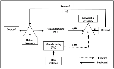
Figure 1. Hybrid manufacturing/remanufacturing system.
The mode of the machine ![]() can be described by a stochastic process
can be described by a stochastic process . Such a machine is available when operational
  and unavailable when it is under repair
 .
.
The operational mode of the system is described by the random vector . Given that the dynamics of each machine is described by a 2-state stochastic process, we define a combined stochastic process
 ; its possible values are determined from the values of
  and
and , as follows:
- Mode 1:  and
and  are operational.
- Mode 2:  is operational and
  is under repair.
- Mode 3:  is under repair and
  is operational.
- Mode 4:  and
and  are under repair.
With ![]() denoting a jump rate of the system from state
denoting a jump rate of the system from state ![]() to state
to state![]() , we can describe
, we can describe  statistically by the following state probabilities:
 (1)
(1)
where ,
,  and
and  for all
 ![]()
The transition diagram, which describes the dynamics of the considered manufacturing system, is presented in Figure 2, with:  (failure rate of
 ),
),  (failure rate of
 ),
),  (corrective maintenance rate of
 ) and
) and  (corrective maintenance rate of
 ).
).
The dynamics of the system is described by a discrete element, namely , and continuous elements
  and
and . The discrete element represents the status of the machines and the continuous one, the stock level of serviceable inventories and returned items. The stock level
  can be positive for an inventory or negative for a backlog. We assume that there is no shortage of returned products, then
 .
.
We assume that the failure rate of  depends on its production rate, and is defined by:

Hence,  is described by the following matrix:
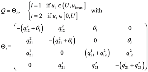 (2)
(2)
 (a)
(a) (b)
(b)
Figure 2. States transition diagram. (a) Each machine; (b) The system.

Let  and
and  denote the production rates of the machines
  and
and , respectively. The set of the feasible control policies
 , including
  and
and , is given by:
 (3)
(3)
where  and
and  are known as control variables, and constitute the control policies of the problem under study. The maximal productivities of the manufacturing machine and the remanufacturing machine are denoted by
  and
and , respectively.
The continuous part of the system dynamics is described by the following differential equations:
 (4)
(4)
 (5)
(5)
where  and
and ![]() are the given initial stock level of serviceable inventories and returned items, return rate, disposal rate and demand rate, respectively.
are the given initial stock level of serviceable inventories and returned items, return rate, disposal rate and demand rate, respectively.
Let  be the cost rate defined as follows:
![]() (6)
(6)
where constants  and
and  are used to penalize the serviceable inventory and backlog, and inventory of returns, respectively. The holding and backlog costs are such that
![]()
![]() .
.
The production planning problem considered in this paper involves the determination of the optimal control policies (![]() and
and![]() ) minimizing the expected discounted cost
) minimizing the expected discounted cost  given by:
 (7)
(7)
where ![]() is the discount rate. The value function of such a problem is defined as follows:
is the discount rate. The value function of such a problem is defined as follows:
 (8)
(8)
Based on the value function presented in (8), the optimality conditions and the numerical methods used to solve them (in order to determine the optimal manufacturing and remanufacturing rates) are presented in Appendix A.
The next section provides a numerical example to illustrate the structure of the control policies.
4. Analysis of Results and Sensitivity Analysis
Here, we illustrate the resolution of the model above with a numerical example. Sensitivity analyses with respect to the system parameters are also presented to illustrate the importance and effectiveness of the proposed methodology.
4.1. Optimal Control Results of Numerical Illustration
This section gives a numerical example for a hybrid manufacturing/remanufacturing system presented in Section 3.
The considered computation domain ![]() is given by:
is given by:
 (9)
(9)
The production system will be able to meet the demand rate over an infinite horizon and reach a steady state if the following condition is satisfied: . With
  and
and and the data presented in Table 1,
  and
and . The condition for meeting customer demand is also satisfied with
  because
 .
.
The production policies, illustrated in Figure 3 and Figure 4 indicate the production rates of  for a given stock of return products
  and stock level
 . Based on the results, there is no need to produce at a comfortable stock level capable of meeting demand; we do not need to produce if the stock level is greater than 7.5 and 10.5 parts at modes 1 and 2, respectively. Unlike the case illustrated in Figure 3, where the tendency was to use the maximal productivity of
  less at mode 1, the first threshold in Figure 4 is higher than in Figure 3 because the machine works alone.
Figure 5 and Figure 6 illustrate the optimal production rate boundary of  at mode 1 and mode 2, which is the optimal stock level, such that even with stock levels below 7.5 and 10.5, we need to produce at the economical and at the maximum production rates. If the stock of the return product increases, the stock level de-
Figure 3. Production rate of ![]() at mode 1.
at mode 1.

Table 1. Numerical data of the considered system.
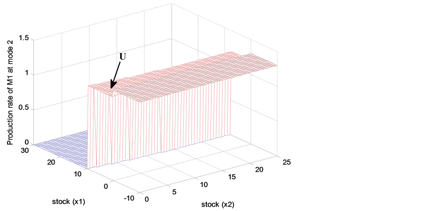
Figure 4. Production rate of ![]() at mode 2.
at mode 2.
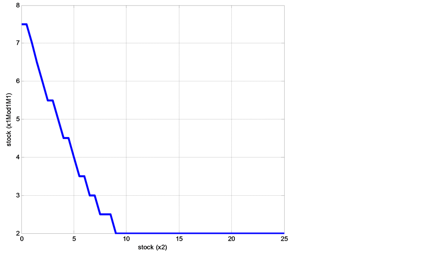
Figure 5. Boundary of ![]() at mode 1.
at mode 1.
creases. The traces of  at mode 1 (Figure 5) and mode 2 (Figure 6) show that for a quantity of returned products greater than 9 (12.5), regardless of the level of serviceable stock, the production rate will need to be set to its maximal rate.
According to the classical results as in [8] and [9] , and references therein, the computational domain is expected to be divided into two stages. The results of Figure 3 and Figure 4 show however that the computational domain is divided into three stages, which represents a specific finding of this paper.
Examining Figures 3 to 6, we see that the optimal stock levels depend directly on the level of returned products. Consequently, the optimal production control policy consists of one of the following rules:
1) Set the productivity of  to its maximal value when the current stock level is under the first threshold value (
 and
and , respectively);
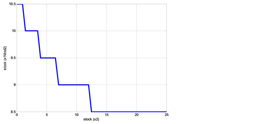
Figure 6. Boundary of ![]() at mode 2.
at mode 2.
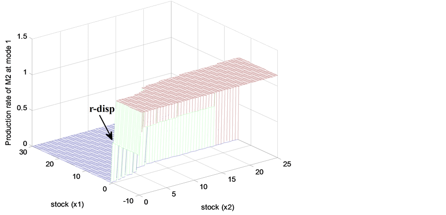
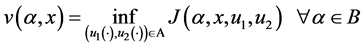
Figure 7. Production rate of ![]() at mode 1.
at mode 1.
2) Reduce the productivity of  to its economical value when the current stock level approaches the second threshold value (
 and
and , respectively);
3) Set the productivity of  to zero when the current stock level is greater than the second threshold value.
4) In Figures 7-10, the optimal policies of  at mode 1 and mode 3 are presented. At mode 3, the zone where the machine is set to its maximal production rate is larger than that at mode 1. This illustrates the difference between operational modes 1 and 3. The gap between states 1 and 3 is due to the fact that at mode 3, the manufacturing machine is under repair and the remanufacturing machine cannot satisfy the customer demand alone.
5) The relation between the inventory, the stock of returned products and the production rate of  at operational mode 1 (mode 3) is illustrated in Figure 7 (Figure 8). The results show that when the stock level is greater than 5.5 parts (19 parts) and the stock of returned products is greater than 8.5 parts (less than 10 parts), the production rate is set to zero. If the stock level is less than 1 part (17 parts), the production rate is set to its maximal value. The results of Figure 7 show that the zone where the production rate is set to zero is restricted when the stock of returned products increases. The effect of a large quantity of
 ![]() is minimized by assigning large values of the stock threshold at mode 1. In Figure 7 and Figure 8, we can see that for
is minimized by assigning large values of the stock threshold at mode 1. In Figure 7 and Figure 8, we can see that for , the production rate of
  is set to
  (see zone T).
Figure 9 (Figure 10) illustrates the optimal production rate boundary of  at mode 1 (mode 3), which is the optimal stock level. The results show that the threshold values also depend on the level of returned products.
The computational domain of  at mode 1 and 3 is divided into two regions where the optimal production control policy consists of the following two rules:
1) Produce at the maximal rate (or at  if
if ) when the current stock level is under a threshold value (
 and
and , respectively).
2) Set the production rate to zero when the current stock level is larger than a threshold value.
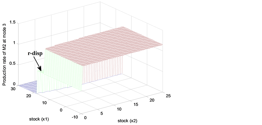
Figure 8. Production rate of ![]() at mode 3.
at mode 3.

Figure 9. Boundary of ![]() at mode 1.
at mode 1.
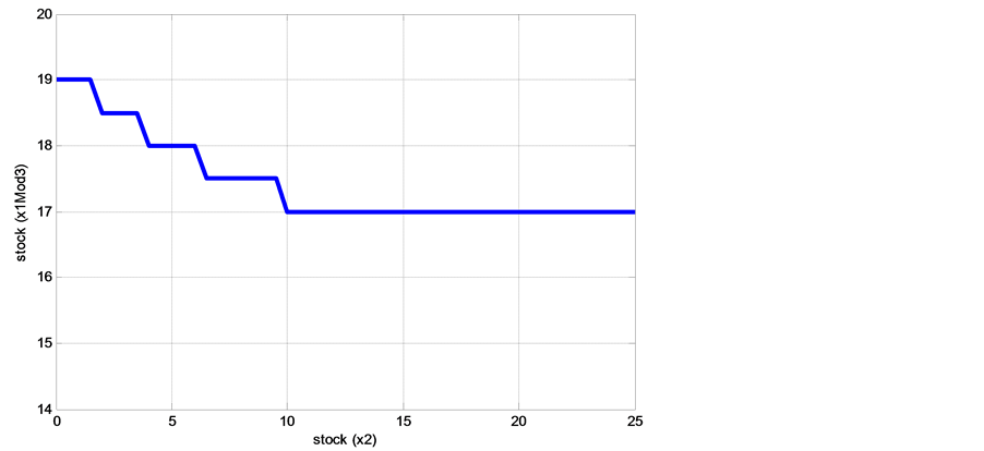
Figure 10. Boundary of ![]() at mode 3.
at mode 3.
3) The results of Figure 8 show that the threshold value  is higher than the thresholds
  and
and  because at mode 3,
  is under repair. The second machine must use its maximum productivity over a long period to avoid over-shortages.
The results of Figure 10 show that at mode 3 where  is under repair, when
 ![]() increases,
increases,  decreases because
  cannot satisfy the customer demand alone. At mode 2, where
  is under repair, we still have multiple thresholds because with two machines, even if one machine fails, the system knows that it exists, and will return to the operational state in a relatively short time.
Based on the results from Figures 3-10, the production rates of  and
and  are given by a
 ![]() dependent hedging point:
dependent hedging point:
 (10)
(10)
 (11)
(11)
 (12)
(12)
 (13)
(13)
where  and
and  are the first and the second threshold values of
  at mode 1, the first and the second threshold values of
  at mode 2, the optimal threshold value of
  at mode 1 and the optimal threshold value of
  at mode 3, respectively.
With numerical methods, the results show that . Physically, however, the system cannot exceed the value of
  because
  cannot satisfy the customer demand alone. Hence, the threshold value
  will be ignored.
In the hybrid manufacturing/remanufacturing system consisting of two machines and one type of product, with a constant failure rate such as the one described in [8] and [9] , the optimal control policy should be characterized by three threshold values. The results obtained in this paper show that the optimal control policy is characterized by five different threshold parameters:  because the manufacturing machine degrades according to its productivity speed. This is the main finding of this paper.
The optimal policy of the proposed joint optimization of production and machine reliability is given by (10)- (12). To validate and illustrate the usefulness of the developed model, let us confirm the obtained results through a sensitivity analysis. Several experiments were conducted to ensure that the structure of the policies obtained is maintained under the variation of the model parameters, and can therefore be used in practice.
4.2. Sensitivity Analysis
A set of numerical examples were considered to measure the sensitivity of the control policies obtained in mode 1 (both machines are producing) and to illustrate the contribution of this paper. We analyze the sensitivity of the control policies according to the backlog costs in the first section. In the subsequent section, we examine the sensitivity of the optimal policies according to different values of the return rate. The sensitivity analysis enables the tracking of variations to the policy boundaries.
4.3. Sensitivity Analysis with Respect to Backlog Costs
In this section, we will perform sensitivity analysis on the backlog cost.
Figure 11 and Figure 12 illustrate the behavior of the optimal threshold values of the machines for five backlog cost values:  and
and . The results show that the thresholds
  and
and  increase as the backlog costs increase. We therefore need a lot of parts in stock to avoid further backlog costs.
4.4. Sensitivity Analysis with Respect to Return Rate
This section analyzes the sensitivity of the optimal threshold values with respect to the return rates.
When the return rate takes four values: ![]() and
and  (where
 ![]() is the demand rate), we obtain the results presented in Figure 13 and Figure 14. The results show that the variation of the parameter
is the demand rate), we obtain the results presented in Figure 13 and Figure 14. The results show that the variation of the parameter  does not affect the threshold
 .
.
When  increases, the thresholds
  decrease in order to avoid over-stocking. The threshold value
  increases as well because
 ![]() is enough to supply
is enough to supply . From a practical perspective, the parameters of the control policy move as predicted when
  decreases, in order to avoid over-shortages (see Figure 13). Zone T moves in the opposite direction of the return rates. For example, if the return rate increases, zone T will shrink (see Figure 14). Increasing
  means that the value of
  is close to
 . Hence, the production rate
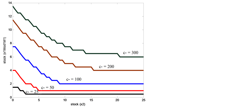
Figure 11. Variation of  at mode 1: Effect on
![]() .
.
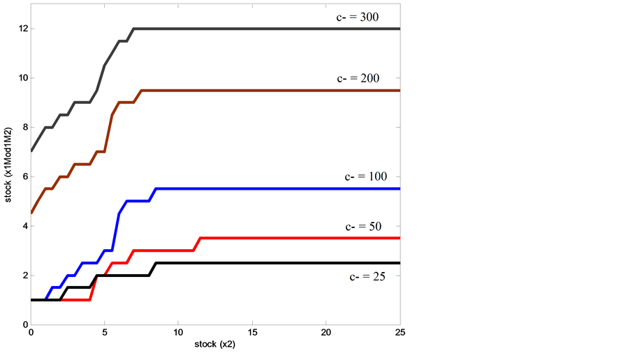
Figure 12. Variation of  at mode 1: Effect on
![]() .
.
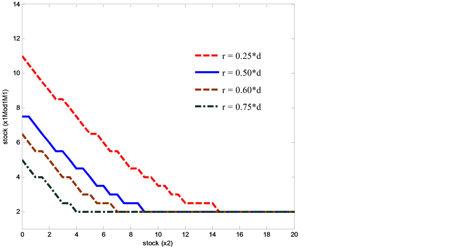
Figure 13. Variation of  at mode 1: Effect on
![]() .
.
of the remanufacturing machine is set directly to its maximal value instead of  as in the base case
 . Zone T moves as predicted, from a practical perspective when
  decreases.
Through the observations drawn from the sensitivity analysis, the results demonstrate conclusively that the resulting policy is optimal and enhances machine reliability. Control policies for our systems consider an extension of the multi-hedging point structure. Without in any way limiting the generality of this proposal, this model is based on certain assumptions relating to a pair of machines (manufacturing and remanufacturing machines) which are not identical and which operate in parallel. Given certain conditions, extended versions of this model might be adopted across a number of industrial sectors.
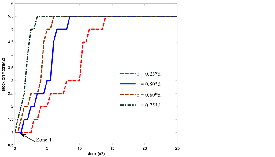
Figure 14. Variation of  at mode 1: Effect on
![]() .
.
5. Conclusions
Although some of the concepts of reverse logistics, such as the facility location models including return flows, inventory management models, production and transportation planning models, have been put into practice for years, it is only fairly recently that the integration of aspects related to the stochastic dynamics of machines has been a real concern for the management of reverse logistics systems. This paper confirms that it is possible to integrate production-dependent failure rates in a hybrid manufacturing/remanufacturing system subject to random failures and repairs, in order to minimize the overall incurred cost. The machines produce one type of final product.
The failure rates of the manufacturing machine depend on its production rate. To take into account its availability, the company will then maximize the recovery of its products used from the market, allowing it to eventually minimize the use of raw materials which become increasingly rare. We developed the stochastic optimization model of the considered problem with two decision variables (production rates of manufacturing and remanufacturing machines). The stock levels of new and returned products were the state variables. From the numerical study, it was found that for two parallel machines, when the failure rates of the machines depend on the production rate, the hedging point policies are optimal within a five-threshold feedback policy, and the reliability of the machines is enhanced. A numerical example is given to illustrate the utility of the proposed approach. The sensitivity analyses show that the structure of the results obtained is maintained. This approach takes into account both the multi-objective aspect and the dynamics of machines. However, the model is far from perfect, and leaves much to be desired, especially in the case involving multiple machines, multiple products, random return rate, the quality of remanufactured products (non-conforming products) and the returns control policy, such as the pricing policy.
References
- Kiesmuller, G.P. (2003) A New Approach for Controlling a Hybrid Stochastic Manufac-turing/Remanufacturing System with Inventories and Different Leadtimes. European Journal of Operational Research, 147, 62-71. http://dx.doi.org/10.1016/S0377-2217(02)00351-X
- Aksoy, H.K. and Gupta, S.M. (2005) Buffer Allocation Plan for a Remanu-facturing Cell. Group Technology/Cellular Manufacturing, Elsevier Ltd., Amsterdam.
- Kumar, S. and Putnam, V. (2008) Cradle to Cradle: Reverse Logistics Strategies and Opportunities across Three Industry Sectors. International Journal of Production Economics, 115, 305-315. http://dx.doi.org/10.1016/j.ijpe.2007.11.015
- Esterman, M., Gerst, P., DeBartolo, E. and Haselkorn, M. (2006) Reliability Pre-diction of a Remanufactured Product: A Welding Repair Process Case Study. 2006 ASME International Mechanical Engineering Congress and Exposition, IMECE2006, 5-10 November 2006, Chicago,
- Min, H. and Ko, H.-J. (2008) The Dynamic Design of a Reverse Logistics Network from the Perspective of Third-Party Logistics Service Providers. International Journal of Production Economics, 113, 176-192. http://dx.doi.org/10.1016/j.ijpe.2007.11.015
- Berthaut, F., Pellerin, R. and Gharbi, A. (2009) Control of a Repair and Overhaul System with Probabilistic Parts Availability. Production Planning and Control, 20, 57-67. http://dx.doi.org/10.1016/j.ijpe.2007.11.015
- Zhang, T.Z., Wang, X.P., Chu, J.W. and Cui, P.F. (2010) Remanufacturing Mode and Its Reliability for the Design of Automotive Products. 5th International Conference on Responsive Manufacturing—Green Man-ufacturing (ICRM 2010), Ningbo, 11-13 January 2010, 25-31.
- Kenne, J.-P., Dejax, P. and Gharbi, A. (2012) Production Planning of a Hybrid Manufacturing-Remanufacturing System under Uncertainty within a Closed-Loop Supply Chain. International Journal of Production Economics, 135, 81-93. http://dx.doi.org/10.1016/j.ijpe.2010.10.026
- Ouaret, S., Polotski, V., Kenné, J.-P. and Gharbi, A. (2013) Optimal Production Control of Hybrid Manufacturing/Remanufacturing Failure-Prone Systems under Diffusion-Type Demand. Applied Mathematics, 4, 550-559.
- Hu, J.-Q., Valiki, P. and Yu, G.-X. (1994) Optimality of Hedging Point Policicies in the Production Control of Failure Prone Manufacturing Systems. IEEE Transactions on Automatic Control, 39, 1875-1880. http://dx.doi.org/10.1109/9.317116
- Martinelli, F. (2007) Optimality of a Two-Threshold Feedback Control for a Manufacturing System with a Production Dependent Failure Rate. IEEE Transactions on Automatic Control, 52, 1937-1942. http://dx.doi.org/10.1109/TAC.2007.906229
- Martinelli, F. (2010) Manufacturing Systems with a Production Dependent Failure Rate: Structure of Optimality. IEEE Transactions on Automatic Control, 55, 2401-2406. http://dx.doi.org/10.1109/TAC.2010.2054790
- Kushner, H. (1992) Numerical Methods for Stochastic Control Problems in Con-tinuous Time.
- Gharbi, A., Hajji, A. and Dhouib, K. (2011) Production Rate Control of an Unreliable Manufacturing Cell with Adjustable Capacity. International Journal of Production Research, 49, 6539-6557. http://dx.doi.org/10.1080/00207543.2010.519734
- Dehayem, N.F.I., Kenne, J.P. and Gharbi, A. (2011) Production Planning and Repair/Remplacement Switching Policy for Deteriorating Manufacturing Systems. International Journal of Advanced Manufacturing Technology, 57, 827-840. http://dx.doi.org/10.1007/s00170-011-3327-1
Appendix A. Optimality Conditions and Numerical Approach
This section presents the optimality conditions satisfied by the value function presented in (8). The properties of the value function and the manner in which the Hamilton-Jacobi-Bellman (HJB) equations are obtained can be found in [11] and [12] . Regarding the optimality principle, we can write the HJB equations as follows:
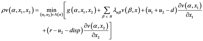 (A.1)
(A.1)
where  and
and  are the partial derivatives of the value functions
  and
and , respectively.
The optimal control policy  denotes a minimizer over
  of the right hand of (A.1). This policy corresponds to the value function described by (8). When the value function is available, an optimal control policy can then be obtained by solving (A.1). The proof of optimality conditions to approximate HJB equations follows the same scheme adopted in [11] and [12] for production planning of a manufacturing system with production-dependent failure rates.
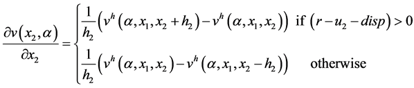
To solve the HJB equations, the numerical method based on the Kushner approach [13] as in [14] and references therein is used. Let ![]() and
and ![]() denote the length of the finite difference interval of the variables
denote the length of the finite difference interval of the variables  and
and![]() , respectively. By approximating
, respectively. By approximating  and
and  by functions
 ![]() and
and![]() , and the first-order partial derivative of the value functions
, and the first-order partial derivative of the value functions  and
and  by:
by:

 The HJB equation becomes:
 (A.2)
(A.2)
where ![]() is the numerical control grid and
is the numerical control grid and 
In this paper, we use the value iteration procedure to approximate the value function given by (A.2). Reference [15] and references therein provide details on such methods.
The discrete dynamic programming (A.2) gives the following six equations:
mode 1
 (A.3)
(A.3)
with 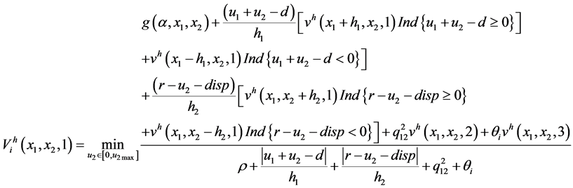
mode 2
 (A.4)
(A.4)
with 
mode 3
 (A.5)
(A.5)
mode 4
 (A.6)
(A.6)
The contribution of this research to the Hamilton-Jacobi-Bellman (HJB) equations lies in the fact that at modes 1 and 2, where  is operational, we have four equations (see (A.3) and (A.4)) instead of two, in the case of a hybrid manufacturing/remanufacturing system without production-dependent failure rates.