Applied Mathematics
Vol. 3 No. 11 (2012) , Article ID: 24521 , 17 pages DOI:10.4236/am.2012.311236
The Discrete Agglomeration Model: Equivalent Problems
West Virginia University, Morgantown, USA
Email: moseley@math.wvu.edu
Received July 22, 2011; revised October 11, 2012; accepted October 18, 2012
Keywords: Agglomeration; Coagulation; Smoluchowski; Differential Equations
ABSTRACT
In this paper we develop equivalent problems for the Discrete Agglomeration Model in the continuous context.
1. Introduction
Agglomeration of particles in a fluid environment (e.g., a chemical reactor or the atmosphere) is an integral part of many industrial processes (e.g., Goldberger [1]) and has been the subject of scientific investigation (e.g., Siegell [2]). A fundamental mathematical problem is the determination of the number of particles of each particle-type as a function of time for a system of particles that may agglutinate during two particle collisions. Little analytical work has been done for systems where particle-type requires several variables. Efforts have focused on particle size (or mass). This allows use of what is often called the coagulation equation which has been well studied in aerosol research (Drake [3]). Original work on this equation was done by Smoluchowski [4]) and it is also referred to as Smoluchowski’s equation. The agglomeration equation is perhaps more descriptive since the term coagulation implies a process carried out until solidification whereas we focus on the agglomeration process; that is, on the determination of a time-varying particle-size distribution even if coagulation is never reached.
In his original work Smoluchowski considered the agglomeration equation in a discrete form. Later it was considered in a continuous form by Mller [5]). In either case, an initial particle-size distribution to specify the initial number of particles for each particle size is needed to complete the initial value problem (IVP). We refer to these as the Discrete Agglomeration Model and the Continuum Agglomeration Model respectively. Solution of either model yields an updated particle-size distribution giving number densities as time progresses. For various conditions, studies of these and more general models include Morganstern [6], Melzak [7], Mcleod [8], Marcus [9], White [10], Spouge [11], Treat [12], McLaughlin, Lamb, and McBride [13], Moseley [14], and Moseley [15].
Let R be the real numbers,  I is a finite, infinite, or semi-infinite open interval}, and for
 ,
,
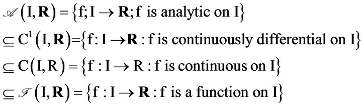
If A is a subspace of a vector space B we write . These function spaces are vector spaces and
To develop the discrete model, assume that all particles are a multiple of a particle of smallest size (volume), say . Thus a particle made up of i smallest-sized particles has size
 . In polymer chemistry, the particle is called an i-mer. The initial time is
  where I0 is the largest time interval of interest. We indicate this by the extended interval notation
 . We also let
  and
and . Unless otherwise specified, we assume
 . Now for each
  let
let  be a real-valued function (either in
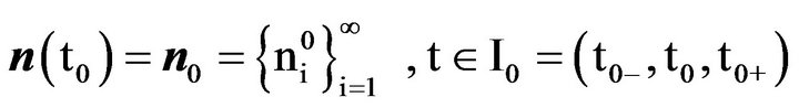
 ) that approximates the number of i-mers in the reactor at time t. Since there are an infinite number of sizes, initially, we take the state (or phase) space to be
 . Assume the initial number density
  is known.
As time passes, particles collide, agglutinations occur, and larger particles result. The net rate of increase in ni(t) with time, dni/dt, is the rate of formation minus the rate of depletion (conservation of mass). For  we consider as a possible Σ space (i.e., the designated space where we look for solutions) either
  for the analytic context or
  for the continuous context where
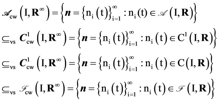
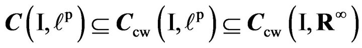
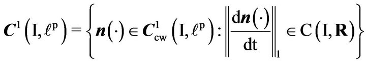
Functions in  are continuous, but functions in
  are not as we have not established a topology on R∞. They are componentwise continuous.
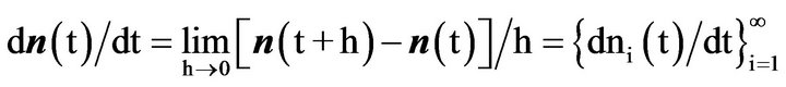
For  we may define
  . The derivatives dni/dt exist and are in C(I,R). However, we can not assert that
  as we have no topology on R∞.
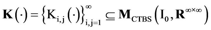
Let  be the set of “infinite matrices”. The kernel (which measures adhesion or “stickiness”),
  , is a doubly infinite array of real-valued functions of time either in
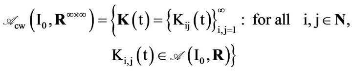
(analytic context) or in
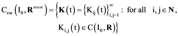
(continuous context). As with , we establish no topology on
 .
.
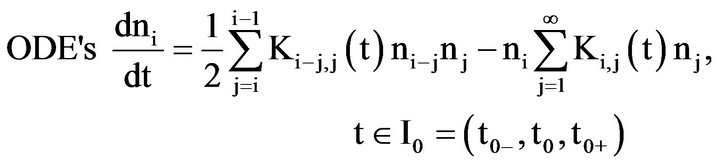
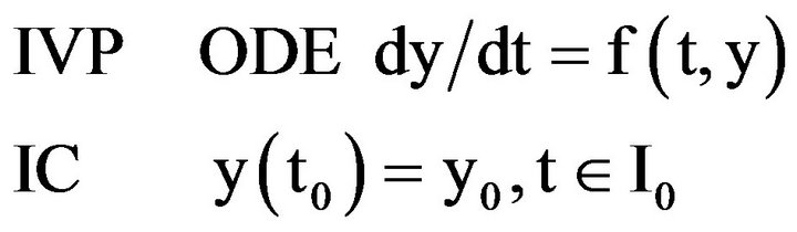
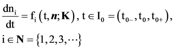
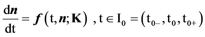
The resultant Discrete Agglomeration Model or Discrete Agglomeration Problem (DAP) is an IVP consisting of an infinite system of Ordinary Differential Equations (ODE’s) each with an Initial Condition (IC) that may be written in scalar (componentwise) form as:
 (1)
(1)
IVP
 (2)
(2)
where for i = 1 the empty sum on the right hand side of (1) is assumed to be zero. The first sum in the scalar (componentwise) discrete agglomeration Equation (1) is the (average) rate of formation of i-mers by agglutinations of  with j-mers. The 1/2 avoids double counting. The second sum is the (average) rate of depletion of i-mers by the agglutinations of i-mers with all particle sizes. We model a stochastic process as deterministic. The physical system is often stationary so that each
  is time independent and the model is said to be autonomous. In a physical context, we require
 . However, we will address DAP as a mathematical problem where we allow the initial number of particles
 , the components of the kernel
 , and the components of the solution,
  , to be negative. The physical context will be a special case.
Smoluchowski found in the physical context that when  is a constant, that
 (3)
(3)
where
 (4)
(4)
uniquely satisfies DAP on its interval of validity
 . If we assume
 , then
 .
.
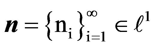
The requirement on  in (4) and the infinite sum in (1.1) motivate consideration of the Banach spaces
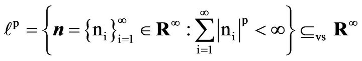 where
where
 (Martin [16, p. 3]) with norm
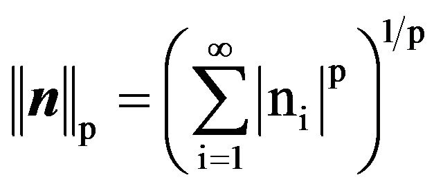
(and hence a metric and a topology). Equality of two vectors in  requires the metric (the norm of their difference) to be zero. This is equivalent to both vectors being in
  and being componentwise equal. If
  , then
 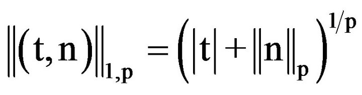 defines a norm on
  (Naylor and Sell [17, p. 58]). To insure that
  exists (even for negative initial conditions)we will require
  so that
 .
.
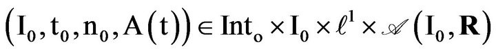
We are particularly interested in the time-varying kernel  which depends on time, but not on particle size. In the continuous context where
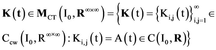
the problem parameters are
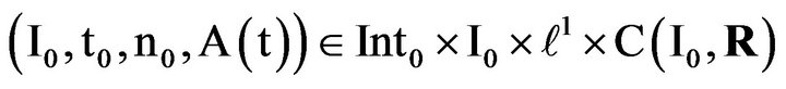 . In the analytic context where
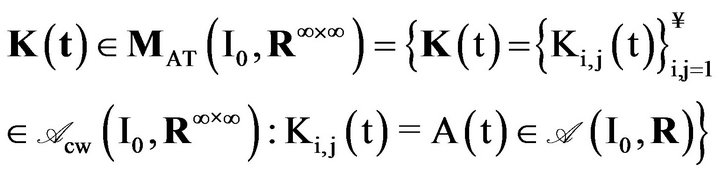
the problem parameters are
 . For any kernel, solution requires that both sides of (1) are continuous in the continuous context and analytic in the analytic context.
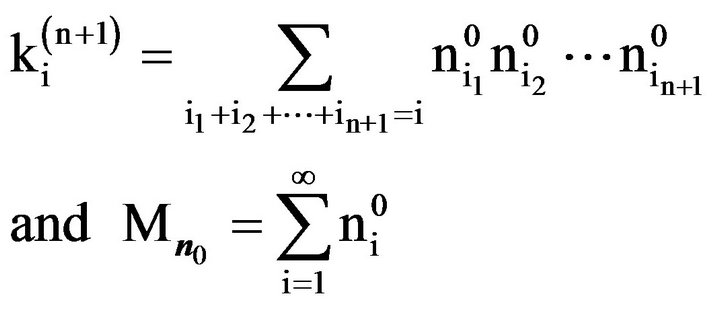
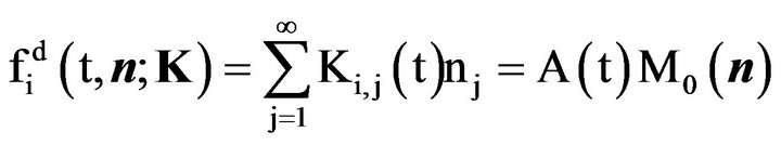
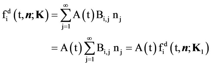
The ith depletion coefficient associated with  and the distribution
  is defined formally by the infinite series
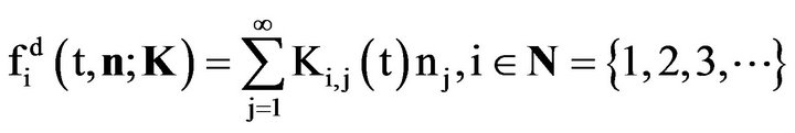 (5)
(5)
The only direct dependence of  on t is through
 . If (5) converges for all
 , then
  maps
maps  to
to . We may view
  as a function of an infinite number of real variables or as a function of time and a size distribution. Regardless, if
 , and we have convergence, the composition
  maps I to R.
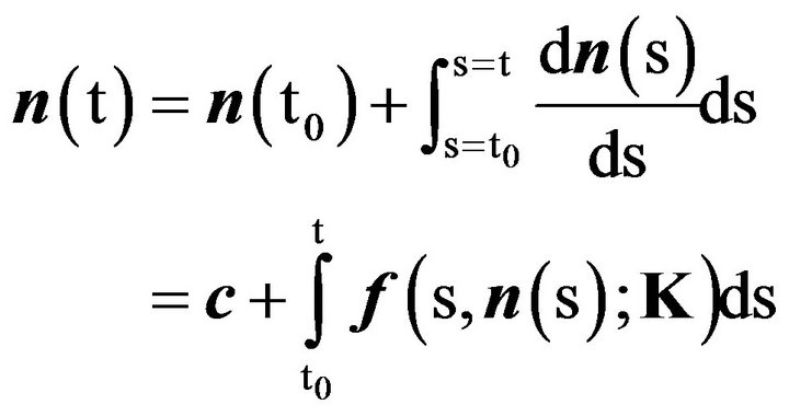
Implicit in (1) is that for solution in the continuous context, we must have for all , that
  . That is, DAP requires us to first find
  such that for all
  and
and ,
,  exists (i.e., converges) and defines a function in
 . If, in addition,
  (the Σ space) and satisfies (1) on I and (2), then it solves DAP on I. This formulation of DAP does not require mathematics beyond calculus and is often used by engineers and scientists.
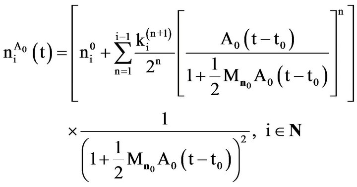
For DAP with a time varying kernel,  , in the analytic context, Moseley [14] established that the more general formula
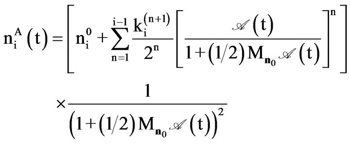 (6)
(6)
where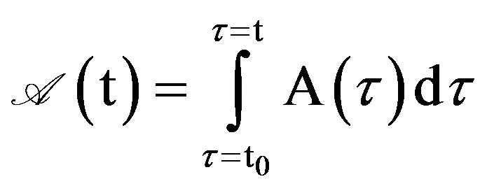 , satisfies DAP uniquely on its interval of validity
 or the physical context where
 , again we have
  and require
  . The formula (6) satisfies (1) on I and (2) in the continuous context as well where we now allow
  However, since (6) was not derived using equivalent equation operations, uniqueness has not been proved rigorously for
  . Unless otherwise stated, for the rest of the paper, we focus on the continuous context.
Moseley [14] divided DAP into several problems which could be considered separately. Under certain conditions, a reasonably complicated change of (both the independent and dependent) variables transforms DAP with a time varying kernel (Moseley, [14]) into another IVP which Moseley later referred to as the Fundamental Agglomeration Problem (FAP). The solution process for FAP is fully documented in Moseley [15]. For FAP, Moseley established existence and uniqueness for both the analytic and continuous contexts by using a sequential solution. To facilitate further progress, in this paper we develop equivalent problems for DAP in the continuous context. Analogs for the analytic context can be obtained.
To rearrange terms in infinite series we will need
 (7)
(7)
If all sums exist, we add all of the elements in  in two different ways. Since we use them often, we will use
  to mean “for all” and
  to mean “there exists” (with apologies to the logicians). If y = n(t), we use any of n, n(t), y(t) and n(
 ) to denote the function. Also, we denote the restriction of a function to a smaller domain by the same symbol. The context will make it clear.
2. Mathematical Problem Solving
Often, a mathematical problem is specified by giving a condition (or conditions) (e.g., an algebraic equation or an ODE with an initial condition) on elements in a Σ set (the designated set where we look for solutions, e.g., ). If the
  set is a vector space, we say Σ space. A problem is (set-theoretically) well-posed if it has exactly one solution in its
  set. (In this paper, we will not consider continuity with respect to problem parameters.) A well-developed model of dynamics using an IVP is well-posed (exactly one event happens). As modelers, we expect our models to be well-posed. As mathematicians, we require rigorous proof. Often, we solve equations by using equivalent equation operations to isolate the unknown(s). This yields uniqueness, and, as all steps are reversible, existence. (Squaring both sides of an equation is not an equivalent equation operation and may lead to extraneous roots.) For linear ODE’s, we may guess the form of a solution and prove existence and uniqueness by using the linear theory. For nonlinear problems, we may prove existence by substituting back into the equation. Uniqueness then becomes an issue.
Let . If a solution is unique in B, and it is in A, then it is unique in A. If A is the Σ set for the problem and contains only one solution, then the solution is unique in B. Being in A is a requirement for existence. In the continuous context, for
 , we look for solutions to
 (8)
(8)
in the  space
space . Thus, as is usually done, we require solutions to (8) to not only exist, but to also have continuous derivatives. We also require
  where
where  and the range of y(t) is in U for y(t) in the
  space. Placing these additional constraints avoids dealing with pathology, but narrows the space where a known solution is to be shown to be unique. There may be (pathological) solutions to (8) where the derivative exists, but is not continuous.
Also, as is usually done, we allow I to vary. If we show that there exists a solution for some I, then we say that we have local existence on I. The largest  where a solution exists is the interval of validity for the solution (i.e., the domain). We say that we have shown global existence on I if, given
  , we prove that there exists a solution on I (i.e., a solution in
 ). Suppose a solution on
  goes through the point where
 . It is said to be locally unique at
  if there exists
  such that it is the only solution on I1. It is locally unique on I if it is locally unique at every point in I. Obviously, if a solution exists globally on
  , and is locally unique on I, then it is globally unique on I. That is, it is the only solution in the
  space
space ).
).
For DAP in the continuous context we start with the large  space
space  and say that
 satisfies (1) on I if
 , the composition
  exists (converges) and is in
  and ni(t) satisfies (1) on I. Since composition of continuous functions is continuous, we expect
  if in some sense
  from
from  given by (5) is continuous. But we do not have a topology on
  and hence not one on
 . Instead of requiring
 ,
,  as a separate condition for solution, we may incorporate it into the Σ space. We refer to DAP with the Σ space
as the Scalar Discrete Agglomeration Problem (SDAP). Obviously, this may be formulated in an analytic context as well.
Recalling the constraint 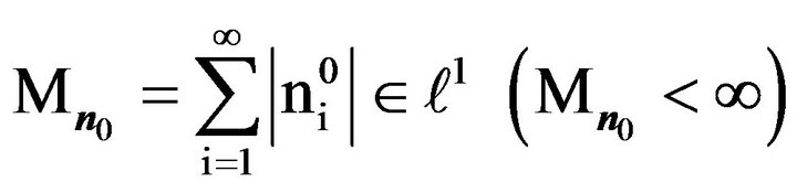 , instead of
 , we may choose the state space as
  which has a norm (and hence a metric and a topology). A solution on I is then a time-varying infinite-dimensional “state vector”
 . Later we will choose an appropriate
  space and write DAP in vector form. We refer to this formulation of DAP as the Vector Discrete Agglomeration Problem (VDAP). As with SDAP, VDAP may be in the continuous or analytic context. If SDAP is well-posed, and its solution is in the (smaller)
  space for VDAP, then SDAP and VDAP are equivalent except for the space where local uniqueness is proved. That is, by choosing a smaller
  space, VDAP requires proving local uniqueness in a smaller space than does SDAP. If we do not worry about pathology, and redefine the
  space for SDAP to be the same as for VDAP, the two problems are equivalent. The question is: How do we choose an appropriate (smaller)
  space? But first we consider an equivalent scalar problem and
  spaces.
2.1. Equivalent Scalar Problems
Again assume for  that
that  converges
  where
where . Now define the functions
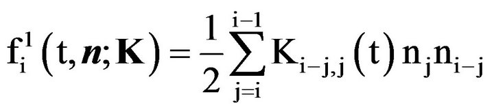 (9)
(9)
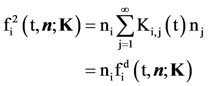 (10)
(10)
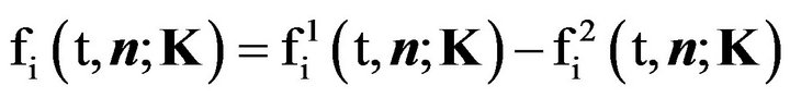 (11)
(11)
which also map . For these functions, as with
  the only explicit dependence on t is through
 . For
. For  we may now write (1) as the system of ODE’s
 (12)
(12)
If the restriction of  to
to  (which we denote by the same symbol) converges
  and is continuous on
  with respect to the norm topology, we write
 . That is,
  .
.
Initially, we assume  and investigate
 , and
, and . Note
  is just a finite sum involving Ki,j(t) and components of
 ,
,  is just the product of
  with a component of
 , and
, and  is just the difference of
  and
and .
.
Theorem 2.1. Let  and
and  . Then
 ,
,  , and
, and  are all in
 .
.
Proof. Sums, products, and compositions of continuous functions involving ℓ1 are continuous. ■
Detailed ε-δ proofs follow proofs in an elementary real analysis course. All functions map to R. We must choose  sufficiently small so that
 . For example, if
  , then the projection function
  is continuous since if
 , then
 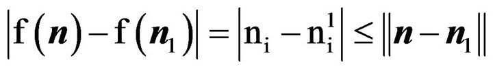 satisfies a Lipschitz condition (Bartle [18, p. 161]) and hence is continuous on ℓ1 i.e., is in
 . Since it is a constant function of t, it is in
 . We investigate continuity and differentiability in ℓp in more detail in the next section.
Let . If the composition
  converges
  and is continuous on I, we write
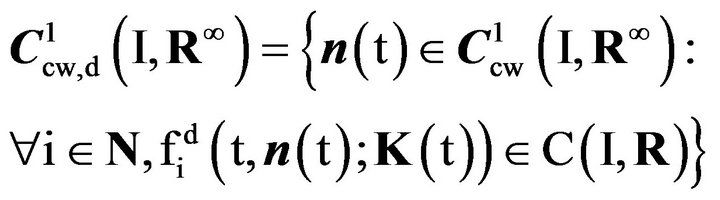
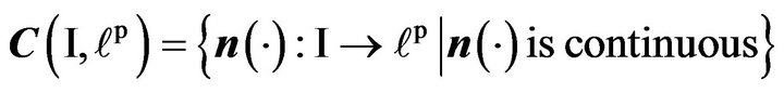
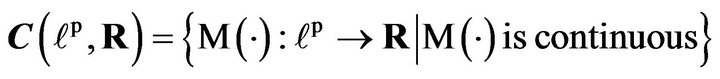
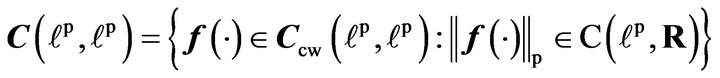
 . Previewing the next section, we define the function spaces
 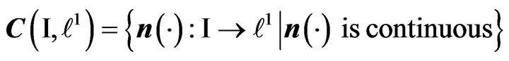 and
and  as the componentwise continuous functions that have codomain ℓ1, and claim that
 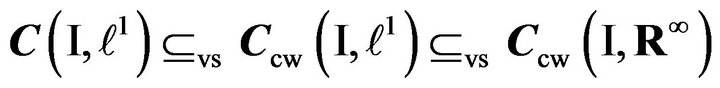 .
.
Corollary 2.2. Let  and
and  . If
. If , then the compositions
  and
and  are all in
 .
.
Proof. Sums, products, and compositions of continuous functions involving  are continuous. ■
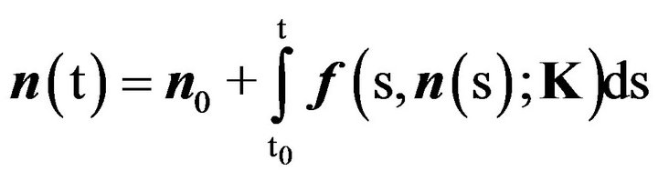
We now show that in the continuous context if  , then SDAP given by (12) and
(2) with the Σ space  is equivalent to the infinite system of scalar (componentwise) Voltera integral equations
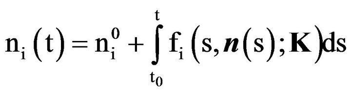 (13)
(13)
where  is a solution to (13) if it is in the
  space
space
and ,
,  satisfies (6). (We require
 and not just that the integral in (6)
exists.) We refer to this problem as the Integral Scalar Discrete Agglomeration Problem (ISDAP) in the continuous context. A formulation in the analytic context can also be established.
Theorem 2.3. In the continuous context, a distribution
 is a solution of SDAP in
  if and only if it is a solution of ISDAP in
 .
.
Proof. First assume that  is a solution of SDAP in
 . We have by the definition of a solution of SDAP, that
 , that
 , that (13) is satisfied on I, and that (2) is satisfied. Since both sides of (13) are continuous, we may integrate from t0 to
  to obtain
 (14)
(14)
Applying the initial condition we obtain (13). Similarly, let us assume that  is a solution of (13) in
 . Substituting in t0 we obtain (2).
Since , we have
  that
that
 so that the integrand,
 , is continuous. Since ni(t) is written as an integral, it is differentiable so that
 . Differentiating we see that (11) is satisfied. ■
For the scalar Equation (2.1), it is the integral formulation that is used to obtain existence (Picard iterations) and uniqueness using a Lipschitz condition. If we choose to specify  as the
  space for both problems, the problems remain equivalent as any solution to (13) in
  is in fact in
 . That is, there are no solutions to (13) in
 . These results can also be established in the analytic context.
2.2. Continuity and Differentiability for ℓp Spaces
Since  has a norm (and hence a metric) we have a topology on the subspace
  of
of . Many of the limit laws can be extended to
 . For example, if
 and
and , then
 . We also have if
 and
and , then
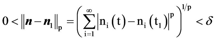
Definition 2.1. A function  is continuous at
  with respect to the norm topology if
 in
in ; that is, given ε > 0,
such that  implies
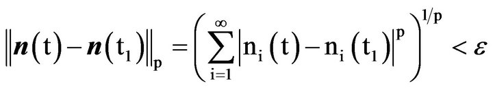 . If it is continuous
 , it is continuous on I. Similarly, a function
  is continuous at
  with respect to the norm topology if
  in I;
in I;
that is, given  such that
 implies
 . If it is continuous
 , it is continuous on
 . Similarly for the functions
 ,
,  , and
, and
 .
.
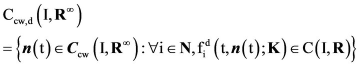
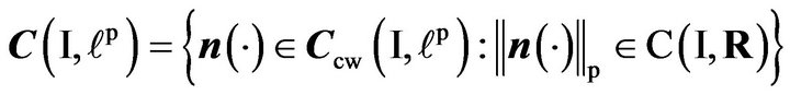
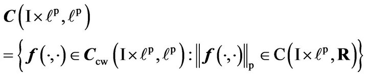
Hence we can define the function spaces
 and
and
 as well as
 ,
,  and
and . If
. If
 , then we may assume
 . For
. For , the range is restricted to the set B whereas, for
 , it is allowed to be in the larger set C. Since
  . However,
  has a norm (and hence a metric and a topology), but
  does not. (We could establish a topology for
 , but this is not necessary if the system states are all in
 .) We will use
  for functions that are componentwise continuous with codomain
  and write
 ,
,
 , and
, and
 . Also, if
 , we write
  if
if ; that is, we use the same symbol for the restriction of a function to a smaller domain.
We give necessary and sufficient conditions for  to be in
  .
.
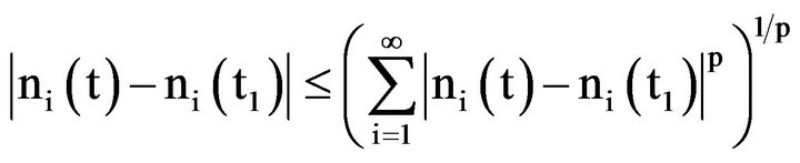
Theorem 2.4. 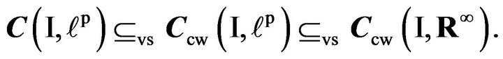 Proof. We show that
 . That is, if
 , then
  is componentwise continuous. As
  is a vector space, by our previous comments
  follows. Let
  and
and . Then
 in
in . That is, given
such that  implies
 . Since
 , given
 such that
  implies
 . Hence
 ,
,  in R so that
 . Hence
 . ■
. ■
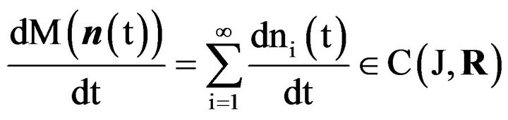
Theorem 2.5. If , then
 .
.
If , then
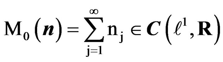 . If
. If , then
 .
.
Proof. If  (or any normed linear space)then the triangle inequality
  implies
 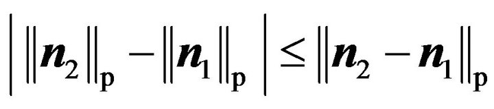 so the norm function
 satisfies a Lipschitz condition on
  and hence is continuous on
  i.e., is in
 . We say it is Lipschitz continuous on
 . Now let
 . Since
  is the composition of the norm function with
 ,
,  implies
 . For
. For , let
, let
 . Since
 ,
, 
exists (converges absolutely). If
 , then so that M0(A) is Lipschitz continuous on
  so that
 .
.
Since the composition of continuous functions (to and from ) is continuous,
Example 2.1. Let  and for
  let
let
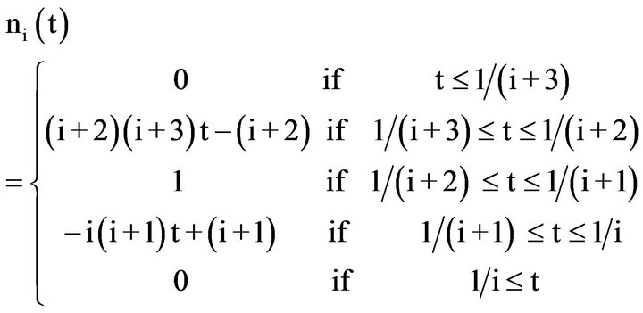 (15)
(15)
Then 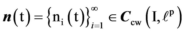 as each ni(t) is continuous and
 ,
,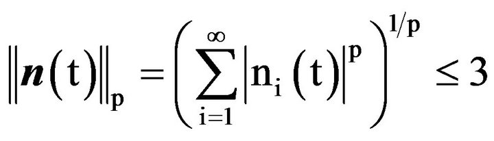 . However,
  ,
,  but for
 ,
, . Hence
  either does not exist or is greater then or equal to 1. Hence
  in not contiuous at
  as
as  does not exist. Hence
  does not exist in
 . Hence
 . Hence the relations
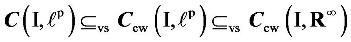 are proper.
Example 2.2. Let  and for any t let
 and
and  otherwise.
Then , we have
  and
and . Obviously
  so
so  even though
  as
as ,
, .
.
Although not sufficient individually for 
to be in , we need its range to be in
 ,
,
 , and
, and . However, all of these do force
  to be in
 .
.
Theorem 2.6.
Proof. Let
 ,
,  ,
, and
and
 .
.
Since ,
,  and
and . Also,
  ,
,  ,
,
and  are all in
 . Let
. Let . Then
 .
.
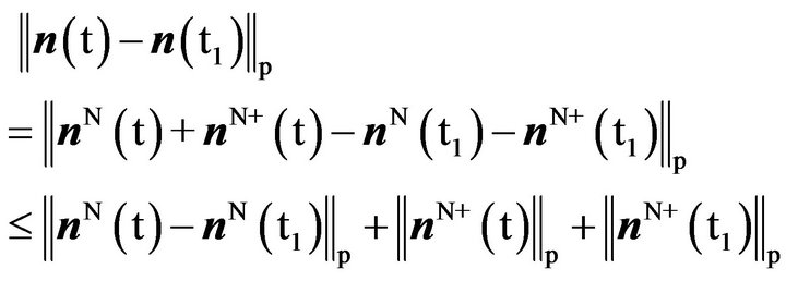
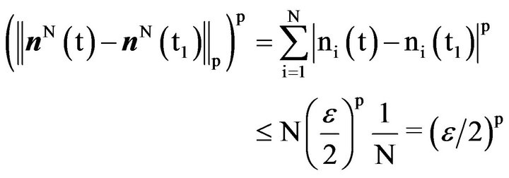
Now let . Since
 , we can choose N sufficiently large so that
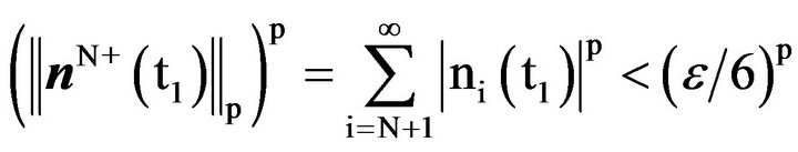 . Since
 ,
,  such that
  implies
  so that
 . Since
 ,
,  choose δi so that
  implies
 . Hence
 .
.
Now choose . Hence
  implies
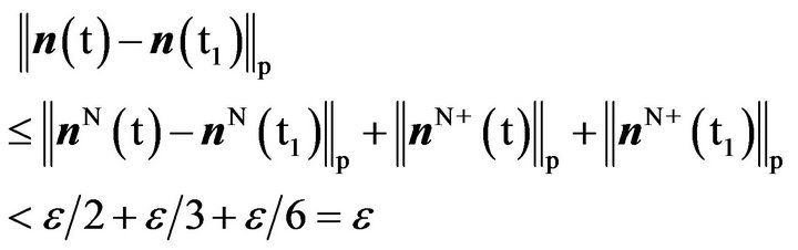 .
.
Hence . ■
. ■
Rather than check directly that , it may be easier to check that for each
 ,
,  ,
,
 since
since  and
and  map from I to R. SimilarlyCorollary 2.7.
 and
and
 .
.
Following the standard proof for products, we also have Theorem 2.8. If  and
and , then
 .
.
Proof. Let  and
and . Choose δ1 such that
 implies
and δ2 such that  implies
 . Let
. Let .
.
Then  implies
■
SimilarlyCorollary 2.9. If  and
and , then
 . If
. If  and
and , then
 . If
. If  and
and , then
 .
.
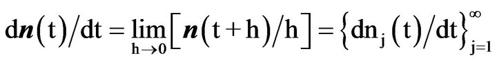
We say  is differentiable
(with respect to the norm topology) at , if
, if
 exists in
 . If
. If  exists
  and is in
 , then
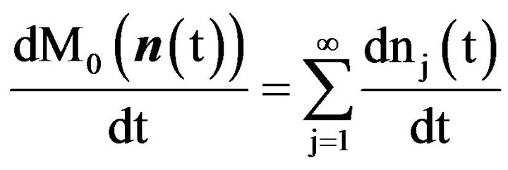
 . We define integration componentwise. Following Theorem 2.6, we have Theorem 2.10. If
 , then
 . Also,
 .
.
Proof. That  follows from considering the limit for components. A proof of
 can be obtained following the proof for scalar valued functions in calculus books (e.g., Stewart [19, p. 88]). The description of
  follows from Theorem 2.6. ■
If at , n(t) has an infinite number of derivatives and equals it’s Taylor series,
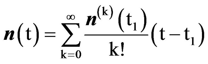
in a neighborhood of t1, it is analytic at t1. If it is analytic
 , then
 .
.
Theorem 2.11.
 ,
,
 ,
,
 ,
,
 ,
,
and
 .
.
Proof. The first containment follows from Theorem 2.10. The remaining proofs are straight forward and often similar to the proof of Theorem 2.4. ■
Theorem 2.12 (Fundamental Theorem of Calculus)
If , then
 , Part 1. (16)
If , then
 . Part 2. (17)
Note that the indefinite integral requires an arbitrary constant vector.
2.3. Kernels, State Spaces and Σ Spaces In the analytic context with an analytic kernel,
 , Moseley [14] used the following procedure to solve DAP. He first established local uniqueness in
  by considering the Taylor series coefficients obtained from the initial conditions and the differential equation. However, he chose a smaller Σ space containing only distributions where if
  is in the Σ space, then
 . He then obtained the explicit formula (6) for the (analytic) solution when A(t) is analytic. He did not rigorously isolate the unknown so he established global existence by showing that the solution given by the formula (6) was in the Σ space, checking the initial conditions (2), and then substituting the formula into (1). Since global existence holds, local uniqueness implies global uniqueness.
The problem of interest is to extend Moseley’s results for the analytic context to the continuous context. The solution given by (6) remains the same except that we now only require . Global existence may be obtained as before. However, local uniqueness is not as easy as it was in the analytic context. McLaughlin, Lamb, and McBride [13] provided local existence and uniqueness for a Continuum Agglomeration Model of linear fragmentation with coagulation as a perturbation using semigroup theory. Spouge [11] provided a local existence theorem in the physical case, but not uniqueness. The standard procedure in Brauer and Noel [20] for a finite dimensional system requires a Lipschitz condition on the right hand side to obtain local existence and local uniqueness. In this paper, we provide preliminaries for using a Lipschitz condition to prove uniqueness in the continuous context by giving equivalent problems in scalar and vector form for DAP with K(t) in a larger collection than
 .
.
Let . If
. If ,
,
 converges
 , then
 maps
maps  to
to . We say that (the restriction of)
  (to
(to ) is in
 if
if , (the restriction of)
 (to
(to ) is in
  and write
 . Furthermore, when
 , we write
 if
if
 .
.
Theorem 2.13. If , and
, and , then
 .
.
Proof. Compositions of continuous functions (in )
)
are continuous so that if  and
and
 , then
 . (See Corollary 2.2.) ■
In the continuous context we wish conditions on  so that
 . Then for
 in (any subspace of)
  we have
 . Then the convergence and continuity condition on
  need not be explicitly stated for the Σ space or as a condition for solution (except as required for interpreting (1)). We begin with three classes of kernels:
 ,
,
 and
and
 .
.
Since  and
and  , if we can prove that for
 , we have
 , then for all kernels in these three classes, if
 , we have
  . However, for clarity, we proceed class by class.
If 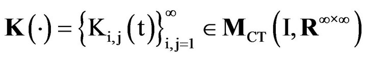 and
and
 , then for all
  we have
 so that
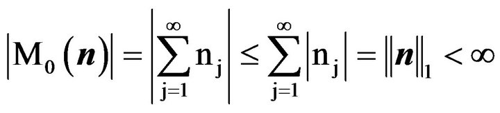
where  is the zeroth moment of the sequence. In the physical context,
  so that,
 is the total number of particles and
  is the total mass of the particles (which should not change) where
  is the first moment of the solution and ρ is the mass density. Treat [12] suggested (as have others) on a physical basis, that these and other moments, possibly all moments, should exist (converge and be continuous). We will take our Σ space as a subspace of
 . Againwe view a solution as a time-varying infinite-dimensional “state vector”
 .
.
Theorem 2.14. Let  so that
 ,
, . If
. If  , then
  exists (converges absolutely) and
 . If
. If , then
exists (converges absolutely) and
 . If
. If , then
  and
and .
.
Proof. Let  so that
 ,
, . By Theorem 2.5, if
 , then
  exists (converges absolutely) and
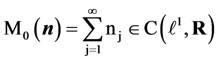 . If
. If , then
  and
and 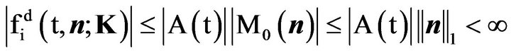 so that
 exists (converges absolutely). By Corollary 2.9,
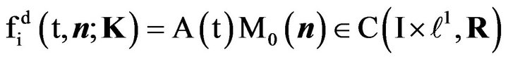 . Now let
 . By Theorem 2.6
  so that
  exists (converges absolutely)
 . Since
 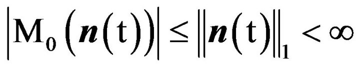 and
and
 ,
,  and
and
 exist (converge absolutely)
 . As compositions and products of continuous functions
(in ) are continuous,
  , and
, and
 are in
 . ■
. ■
Theorem 2.15. Let . Then
 exists (converges absolutely)
and is in . If
. If , then
 .
.
Proof. Let . (Note that
  is a constant function of t for this kernel.) Then
  such that
 . Let
. Let
 and
and . Then
so that  exists (converges absolutely). Now let
 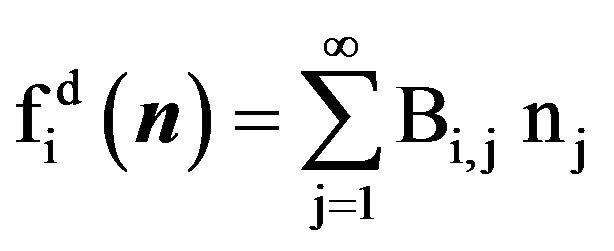 and
and . Then
Hence  is Lipschitz continuous and hence in
 . Since
 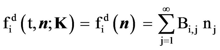 is a constant function of time,
 . Hence
 . If
. If  then
then  and
and
 . ■
. ■
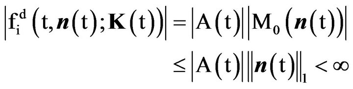
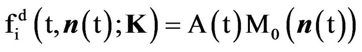
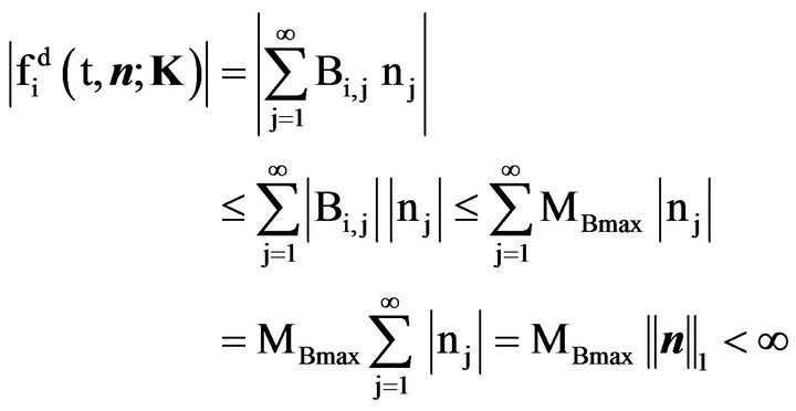
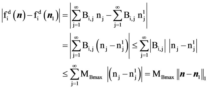
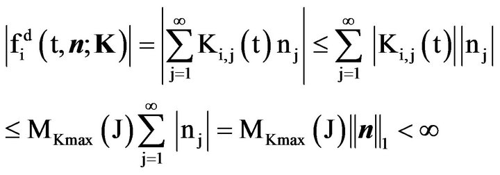
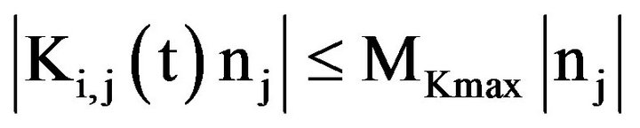
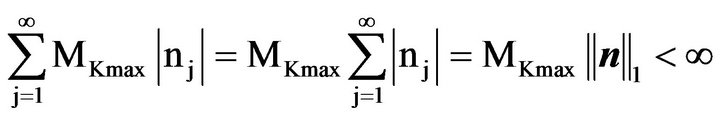
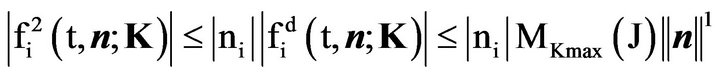
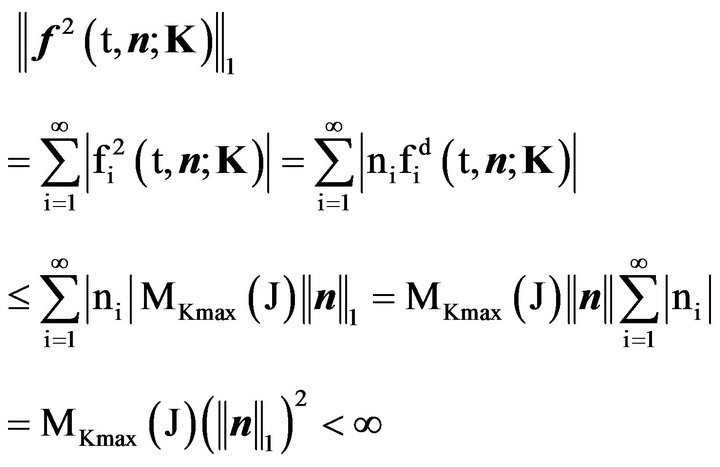
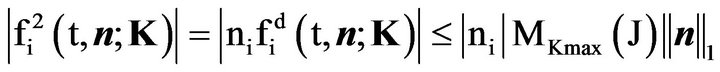
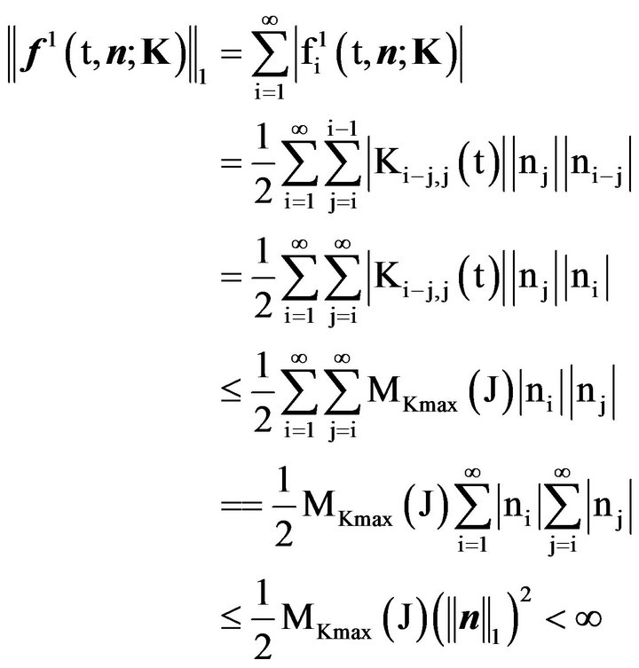
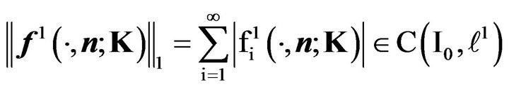
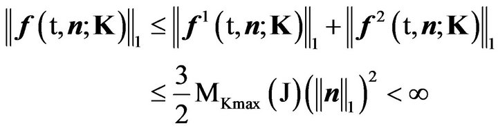
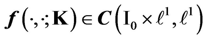
Theorem 2.16. Let . Then
  exists (converges absolutely) and
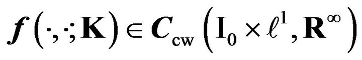 . If
. If , then
 .
.
Proof. Let 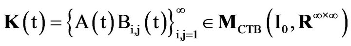
and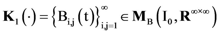 . Then
where  and
and
 (by Theorem 2.15). By Corollary 2.9
 . If
. If , then
 . ■
. ■
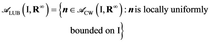
2.4. Weierstrass M-Test and Local Uniform Boundedness Let  and
and . For
. For , let
, let
 . We briefly review the Weierstrass M-test and succeeding theorems on absolute and uniform convergence (Kaplan [21, pp. 436-444]). This should be familiar to engineers and scientists. We then consider a fourth class of kernels. Let
Note  (let
(let
 and
and ). We say that K(t) is locally uniformly bounded in time and size.
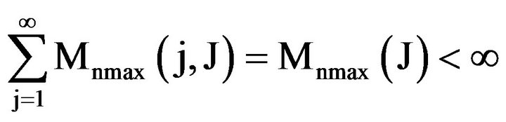
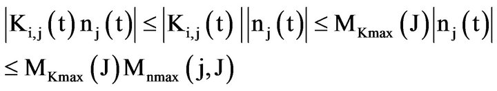
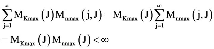
Theorem 2.17 (Weierstrass M-Test Extended). Let
 ,
,  and
and
 . Suppose
 such that
 ,
,  and
and
 , then
 and
and  exist
exist
(converge absolutely  and are uniformly convergent on J so that theyare in
 . Since t1 was arbitrary,
  so
so  and
and  and
and  are in
  so that
 . If
. If  and
and  such that
 ,
,  and
and
 , then
  and
and  exist (converge absolutely)
 and are uniformly convergent on J so that they are in C(J,R). Since t1 was arbitrary,
  so
so  and
and  and
and  are in
  so that
 . Also,
 .
.
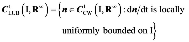
For , to insure
 , we will require
 to satisfy a stronger local uniform boundedness condition in time.
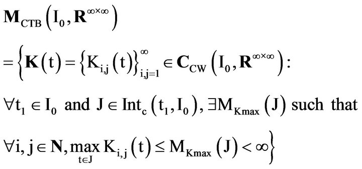
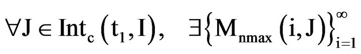
Definition 2.2. Let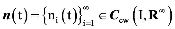 .
.
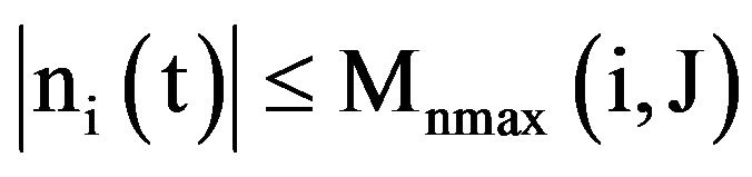
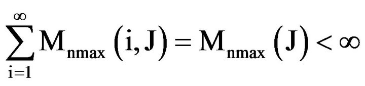
Then  is locally uniformly bounded at t1 if
 , such that
 ,
, 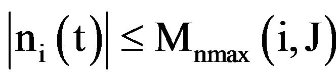 and
and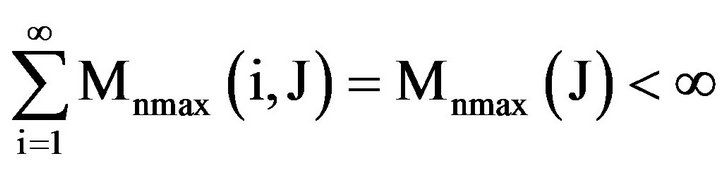 .
.
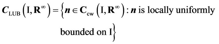
We say  is locally uniformly bounded on I if it is locally uniformly bounded
 .
.
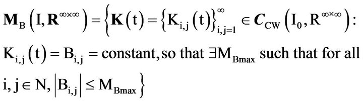
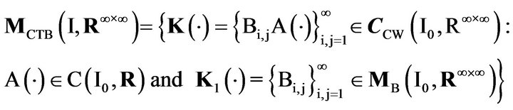
Now let
 ,
,
 and
and
 .
.
Moseley (2007) used  (which he denoted by
 ) as the Σ space in the analytic context. We have
 .
.
Example 2.3. Let  with
with
 and ni(t) increasing. Now for
 , let
, let  and
and
 . Then
 . Hence
 .
.
It can be shown (similar to Moseley [14] in the analytic context) that in the continuous (physical) context,
 where
where  is given by (1.6) is in
  where
where
 .
.
Theorem 2.18. Let
 . Then
  and
and  are in C(I,R) and
 . If
. If  then
then ,
,  and
and
 .
.
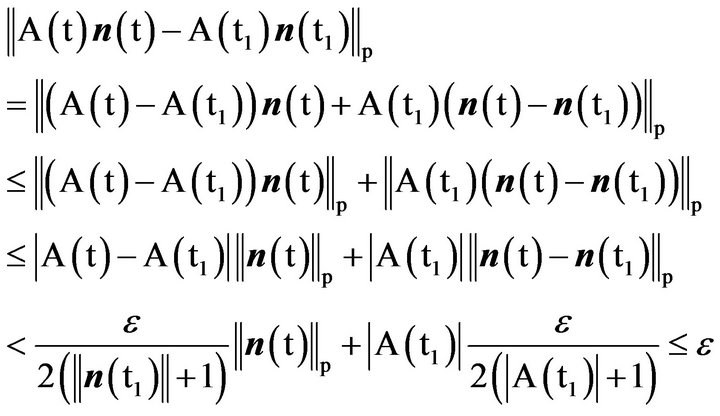
Proof. Let  and
and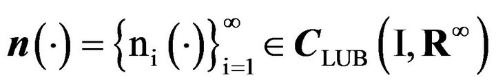 . Then
 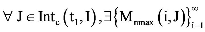 such that
 ,
,  and
and
 . Hence
 ,
,
 so that
 . By Theorem 2.17,
 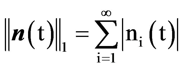 and
and  are in C(J,R). Since t1 was arbitrary,
  and
and 
are in C(I,R). Hence by Theorem 2.6, . If
. If , then, again by Theorem 2.17,
  and
and
 . Hence by Theorem 2.6,
  and so
 . ■
. ■
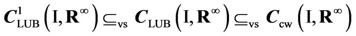
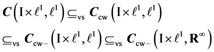
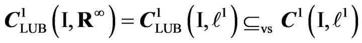
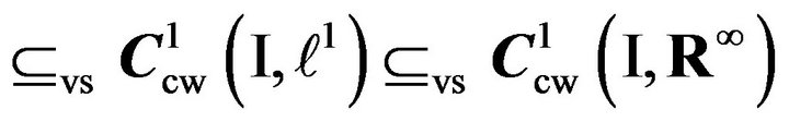
Since the range of functions in  is contained in
 , we have
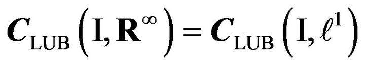 . Similarly,
 .
.
Corollary 2.19.
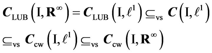 .
.
Also,
 .
.
Proof. By Theorem 2.18, .
.
Everything else is straight forward or follows in a manner similar to the proof of Theorem 2.4. ■
We show that if  and
and
 , then
 . We use the local uniform boundedness of
  and
and . Let
. Let
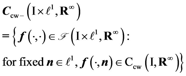
and
Then  and
and  are vector spaces and
Theorem 2.20. Let
 . For
. For , and
, and ,
,  exists (converges absolutely) and
 . If
. If  , then
 .
.
Proof. Let . Then
 , and
, and 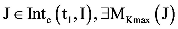 such that for all
  and
and 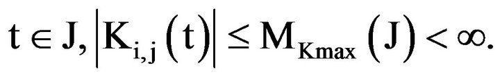 Let
Let  and
and  where
where . Then
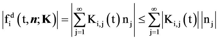
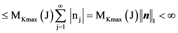 (18)
(18)
so that  exists (converges absolutely for
 ). Since t1 was arbitrary
  exists for
 . Also, since
 and
and
 , by Theorem 2.17 we have that
  and fixed
 ,
, . Hence
 . However, we do not have
 . We may (or may not) be able to prove this with a further extension of the Weirstrauss M-test. Instead we let
 . Then for
  and
and 
 not only do we have
  such that for all
  and
and  but also
  such that
 and
and
 . Then
and
Hence by Theorem 2.17, . Hence
 . ■
. ■
Thus if  and we choose a subspace of
  as our Σ space, we obviate the need to explicitly require
  as a condition for
  to be a solution (except to interpret (1.1)) or as a specific condition for the Σ space.
2.5. Equivalent Vector Problems Recall that if  converges
  the functions
 ,
,  , and
, and  all map
  and that
 maps
maps . Now let
 ,
,
 , and
, and
 . These three functions map
 . As with
 , the only explicit dependence on t is through K(t). If
  and
and , then
 ,
,
 , and
, and  are all in
  (see Theorem 2.1). Now let
  Then by Theorem 2.16,
 . If we can show that
  implies
 ,
,  , and
, and  are in
 , then these functions can be thought of as functions from
  to
to  instead of from
 . We indeed show that if we restrict
  to
to , then the restrictions of
 ,
,  , and
, and  to
to  all map to
  so these functions are all in
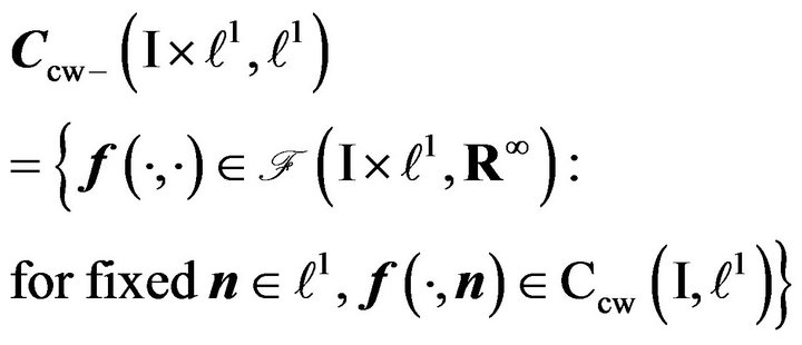
 . Let
. Let
Then  is a vector space. We show that if
 , then
 ,
,  , and
, and  are all in
 . We have
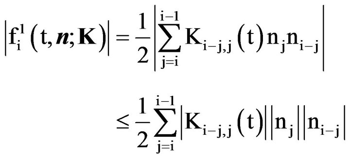
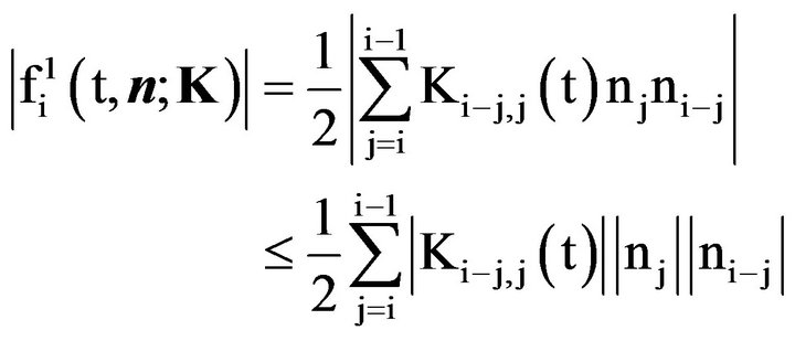
Theorem 2.21. Let . Then, for
 the images
 ,
,  , and
, and  are all in
 . Also,
 ,
,
 , and
, and
 . If
. If
 , the
, the
 , and
, and ,
,
 , and
, and  are all in
 .
.
Proof. Let  and
and . Then
  such that
 . Hence for
  where
where , from (2.12) we have
 so that
and
Since t1 was arbitrary,  ,
,  is in
is in . Furthermore, since
 and
and
 , by Theorem 2.17, for fixed
 ,
,
 .
.
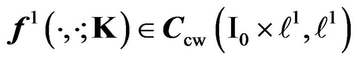
Hence .
.
By Theorem 2.1, . Also, since
we have
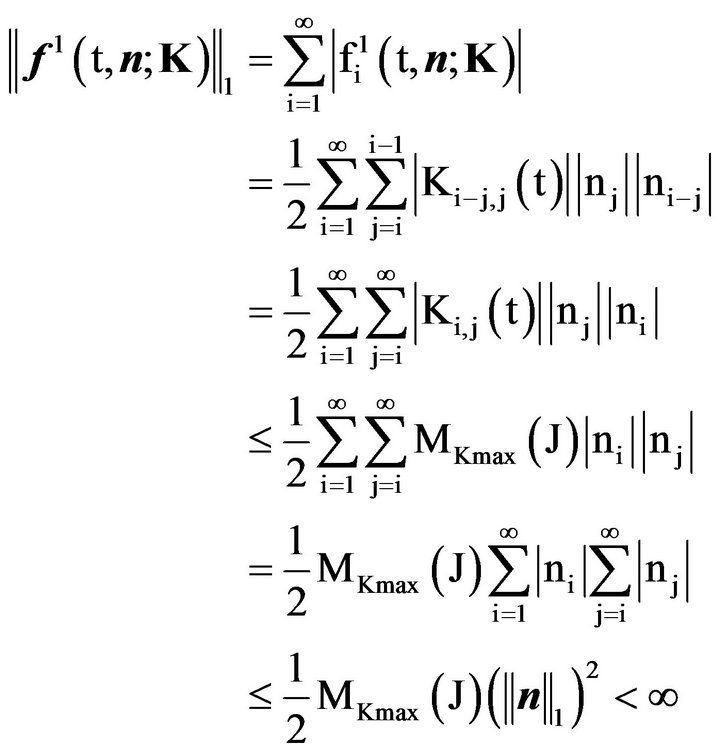
where we have used (7). Hence
 . Since
and
we have for fixed ,
,
 . Hence
 . Since
  is a vector space (note
 )we have that
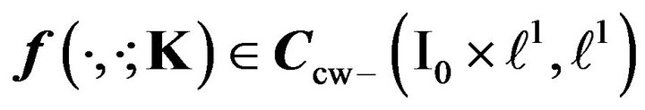 .
.
Now let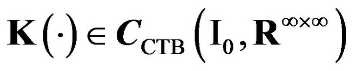 . Then by Theorem 2.16,
 . By using Theorem 2.1 and above,
  ,
,  and
and  are in
Unfortunately, we have not proved that
 . However, assuming
 we consider the Vector Problem (VP):
Vector ODE,
 (19)
(19)
IVP IC
 (20)
(20)
where the derivative and equality are in . That is, we now require the derivative to be defined with respect to the norm topology,
 in
in
 , and equality as equality in
 . For VP, we take our
Σ space as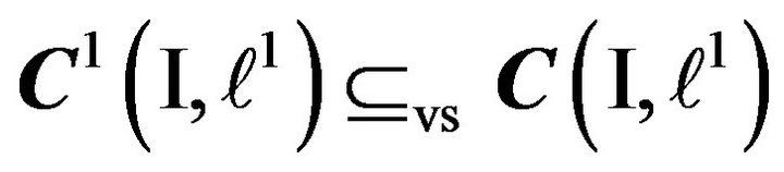 .
.
For  we now show that VP is equivalent to
 (21)
(21)
where for  (the Σ space) to be a solution of (21), we require
 , that (12) holds; that is, integration is componentwise. Equality is in
 . We refer to this problem as the Integral Vector Problem (IVP)
Theorem 2.22. The distribution  is a solution of VP in
  if and only if it is a solution of IVP in
 .
.
Proof. For both problems we have chosen the Σ space to be . Now assume that
  is a solution of VP so that (19) and (20) are satisfied, and the right hand side of (19) is in
 . We may integrate from t0to t using (17) to obtain the vector equation
 (19)
(19)
Applying the initial condition we obtain (21). Now assume that  is a solution of (21). Then substitute
  to obtain (20). Since
 , and
, and
 , differentiating
(componentwise) we have that 
and that (19) holds. ■
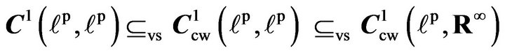
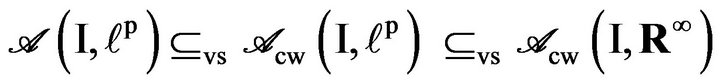
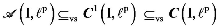
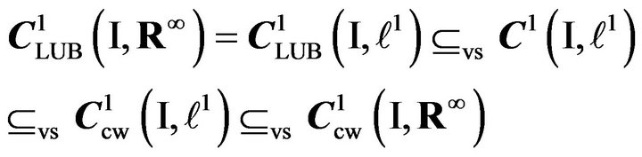
Theorem 2.23. If , then
 and
and
 . If
. If , then
 and
and
 . On the other hand, if
 , then
 and
and
 . If, in addition,
 , then
  and
and .
.
Proof. If , then by Theorem 2.16,
 . By Theorem 2.21,
 . If
. If , then
 and
and
 . Now let
 . Then by Theorem 2.21,
 and
and
 . If, in addition,
 , then
  and
and .
.
To define VDAP in the continuous context, we would like  and
and
 . Then for
 , we would have
  and
and
 . When
 , we do have
 , but have only shown that
  so that for
 , we have
  and
and . We refer to this problem with Σ space
  as VDAP1. When
 , we settle for
 and
and
 so that if
 , then
  and
and
 . We refer to this problem with Σ space
  as VDAP2. As
 , if we take
 as our Σ space for SDAPISDAP, and VDAP1or VDAP2, then they are all equivalent if they have the same problem parameters
 .
.
3. Summary and Future Work For the time-varying kernel ( ) in the analytic context, the problem parameters are
 . For this problem, Moseley [14] used the following problem solving procedure. He first established local uniqueness in
 . However, he chose the smaller Σ space
  containing only distributions where (for a time-varying kernel) if
  is in
is in , then the depletion coefficients
  are in
 , He then obtained the explicit formula (6) for the (analytic) solution. He did not rigorously isolate the unknown so he established global existence by showing that the solution given by the formula (6) was in the Σ space, checking the initial conditions, and then substituting the formula into (1). Since global existence holds, local uniqueness in the analytic context implies global uniqueness.
If we choose  as our Σ space, then SDAP, ISDAP, VDAP1, and IVDAP2 are all equivalent in the continuous context if they have the same problem parameters
 . If
. If
 and
and , we have
 , so that we need not specify this condition separately. For the time varying kernel, the solution given by (6) is in
 where
where  in the continuous context. However, we have not shown (local) uniqueness in the continuous context. To do this we have (at least) four choices:
1) Provide a rigorous derivation of (6) that provides (existence and) uniqueness.
2) Develop and use a Lipschitz condition for:  in the scalar problems SDAP and ISDAP.
3) Extend the (existence and) uniqueness results for FAP in the continuous context to obtain a unique sequential solution to DAP.
4) Develop and use a Lipschitz condition for  in the vector problems VDAP1 and VDAP2.
We have provided preliminaries for the development of a Lipschitz condition for VDAP1 and VDAP2. However, all four alternatives appear to be worthwhile.
REFERENCES
- W. M. Goldberger, “Collection of Fly Ash in a Self-Agglomerating Fluidized Bed Coal Burner,” Proceedings of the ASME Annual Meeting, American Society of Mechanical Engineers, Pittsburg, 1967, 16 pp.
- J. H. Siegell, “Defluidization Phenomena in Fluidized Beds of Sticky Particles at High Temperatures,” Ph.D. Thesis, City University of New York, New York, 1976.
- R. L. Drake, “A General Mathematics Survey of the Coagulation Equation,” In: G. M. Hidy and J. R. Brock, Eds., Topics in Current Aerosol Research, Pergamon Press, New York, 1972.
- M. Von Smoluchowski, “Versuch Einer Mathematichen Theorie der Koagulationskinetik Kollider Lösungen,” Zeitschrift fuer Physikalische Chemie, Vol. 92, No. 2, 1917, pp. 129-168.
- H. Müller, “Zur Allgemeinen Theorie Ser Raschen Koagulation,” Kolloidchemische Beihefte, Vol. 27, No. 6-12, 1928, pp. 223-250.
- D. Morganstern, “Analytical Studies Related to the Maxwell-Boltzmann Equation,” Journal of Rational Mechanics and Analysis, Vol. 4, No. 5, 1955, pp. 533-555.
- Z. A. Melzack, “A Scalar Transport Equation,” Transactions of the American Mathematical Society, Vol. 85, No. 2, 1957, pp. 547-560. doi:10.1090/S0002-9947-1957-0087880-6
- J. B. McLeod, “On a Finite Set of Nonlinear Differential Equations (II),” Quarterly Journal of Mathematics, Vol. 13, No. 1, 1962, pp. 193-205. doi:10.1093/qmath/13.1.193
- A. Marcus, “Unpublished Notes,” Rand Corporation, Santa Monica, 1965.
- W. H. White, “A Global Existence Theorem for Smoluchowski’s Coagulation Equations,” Proceedings of the American Mathematical Society, Vol. 80, No. 2, 1980, pp. 273-276.
- J. L. Spouge, “An Existence Theorem for the Discrete Coagulation-Fragmentation Equations,” Mathematical Proceedings of the Cambridge Philosophical Society, Vol. 96, No. 2, 1984, pp. 351-357. doi:10.1017/S0305004100062253
- R. P. Treat, “An Exact Solution of the Discrete Smoluchowski Equation and Its Correspondence to the Solution in the Continuous Equation,” Journal of Physics A: Mathematical and General, Vol. 23, No. 13, 1990, pp. 3003- 3016. doi:10.1088/0305-4470/23/13/035
- D. J. McLaughlin, W. Lamb and A. C. McBride, “An Existence and Uniqueness Result for a Coagulation and Multi-Fragmentation Equation,” SIAM Journal on Mathematical Analysis, Vol. 28, No. 5, 1997, pp 1173-1190. doi:10.1137/S0036141095291713
- J. L. Moseley, “The Discrete Agglomeration Model with Time Varying Kernel,” Nonlinear Analysis: Real World Applications, Vol. 8, No. 2, 2007, pp. 405-423. doi:10.1016/j.nonrwa.2005.12.001
- J. L. Moseley, “The Discrete Agglomeration Model: The Fundamental Agglomeration Problem with a Time-Varying Kernel,” Far East Journal of Applied Mathematics, Vol. 47, No. 1, 2010, pp. 17-34.
- R. H. Martin, “Nonlinear Operators and Differential Equations in Banach Spaces,” John Wiley & Sons, New York, 1976
- A.W. Naylor and G. R. Sell, “Linear Operator Theory in Engineering and Science,” Holt Rinehart ND Winston, Inc., New York, 1971.
- R. G. Bartle, “The Elements of Real Analysis,” John Wiley & Sons, New York, 1976.
- J. Stewart, “Essential Calculus, Early Transcendentals,” Thomson Brooks/Cole, Independence, 2007
- F. Brauer and J. A. Nohel, “The Qualitative Theory of Ordinary Differential Equations,” W. A. Benjamin, Inc., New York, 1969
- W. Kaplan, “Advanced Calculus,” Addison-Wesley Publishing Company, Redwood City, 1991.