International Journal of Geosciences
Vol. 3 No. 3 (2012) , Article ID: 21175 , 9 pages DOI:10.4236/ijg.2012.33065
Mapping Potential Fishing Grounds in Lake Malawi Using AVHRR and MODIS Satellite Imagery
1Department of Civil Engineering, University of Malawi, The Polytechnic, Blantyre, Malawi
2Department of Fisheries, Monkey Bay Fisheries Research Station, Monkey Bay, Malawi
3Department of Mechanical Engineering, University of Malawi, The Polytechnic, Blantyre, Malawi
Email: *chav0055@umn.edu
Received December 31, 2011; revised March 10, 2012; accepted April 16, 2012
Keywords: Mapping; MODIS; AVHRR; Lake Surface Temperature (LST); Chlorophyll-a
ABSTRACT
This paper discusses a procedure that was developed to delineate potential fishing grounds in Lake Malawi using data on chlorophyll-a concentration derived from Moderate-resolution Imaging Spectroradiometer (MODIS/AQUA) in combination with lake surface temperature (LST) data obtained from Advanced Very High Resolution Radiometer (AVHRR) and MODIS/Terra satellite sensors. The paper draws from findings of studies [1,2] on development of algorithms for estimating chlorophyll-a and lake surface temperature in Lake Malawi from satellite imagery, respectively. To estimate chlorophyll concentration (a proxy for phytoplankton) in Lake Malawi using data from MODIS satellite imagery, in situ measurements of chlorophyll concentration were conducted at three selected sampling stations over the southeastern arm of Lake Malawi concurrent with satellite image acquisitions. These were regressed on chlorophyll-a concentration values obtained from Ocean Color (MODIS/AQUA) Data using SeaWIFS Data Analysis System (SeaDAS) software. From this, an equation for estimating chlorophyll-a concentration in Lake Malawi from MODIS satellite imagery was developed and used for mapping the spatial distribution of chlorophyll-a concentration in the lake. Since Lake Malawi is an oligotrophic lake, with an average value of chlorophyll concentration of 1 μg/L, areas in the lake with relatively high chlorophyll-a concentration were identified as potential locations for the development of the fishery industry. Estimation of lake surface temperature using satellite imagery involved two main activities. Firstly, in situ measurements of lake surface temperature were conducted at the three selected sampling stations over Lake Malawi concurrent with satellite image acquisitions. The second activity involved downloading and processing AVHRR and MODIS/Terra satellite imagery. AVHRR data covered the period September 1997 to February 1998 whereas MODIS/Terra data covered the period May to November, 2006. Both MODIS Land Surface Temperature (MOD11A1) and Ocean Color Sea Surface Temperature (SST) were downloaded from EOS Gateway website and processed into lake surface temperature. Two glass thermometers were used to measure temperature directly from the lake surface at a depth of 0 - 7.0 cm (i.e., skin temperature) and the average of the two readings was recorded as the lake surface temperature at a particular sampling station. Observed temperatures were regressed on remotely sensed data. ER Mapper was employed in drawing maps showing the distribution of lake surface temperature using the regression equation that was developed. Upwelling and downwelling zones were demarcated from lake surface temperature maps. Upwelling zones were identified as areas with a high potential for the development of the fishery industry because of their association with primary productivity. Using a simple overlay technique, data from both the spatial and temporal distribution of chlorophyll-a and lake surface temperature were used to delineate potential fishing grounds in Lake Malawi. The zone extending from Salima up to the northern part of Nkhotakota and the area on the northeastern tip of Lake Malawi were identified as areas of high primary productivity and therefore potential fishing grounds. These areas generally exhibit persistent cool surface waters, indicative of upwelling; and have relatively abundant phytoplankton.
1. Introduction
In Malawi, 70% of the animal protein uptake by the citizenry is derived from fish [3]; and the largest volume of fish-catch is harvested from Lake Malawi. In the light of the above, the delineation of potential fishing grounds in Lake Malawi would enable the Government to target such areas for the development of the fishery industry thereby boosting fish production for domestic consumption and export. Information on the spatial and temporal distribution of phytoplankton and lake surface temperature (LST) are key in the delineation of areas in the lake with high primary productivity and hence potential fishing grounds. However, conducting in situ measurements of chlorophyll-a concentration (a proxy for phytoplankton) and lake surface temperature over the entire length and breadth of Lake Malawi is a very difficult task because of the large size of the lake, estimated to be 29,743 km2. Hence, satellite remote sensing technology, which provides the desired spatial and temporal resolution to monitor the distribution of chlorophyll-a concentration and lake surface temperature is an attractive option.
The distribution of chlorophyll-a concentration in Lake Malawi (Figure 1) is generally very low and remarkably uniform, both temporally and spatially, with a mean value of 1 μg per liter [4-6]. Areas in the lake with slightly higher concentrations of chlorophyll-a than 1 μg per liter may thus be indicative of abundant phytoplankton. Phytoplankton occupy the base of food webs in water bodies, providing organic matter for all trophic transformations. Fish generally flourish where phytoplankton are abundant. In this regard, the location of potential fishing grounds in a given water body may be identified through maps of phytoplankton distribution.
It should be pointed out at the outset that certain types of algae blooms, e.g. so-called harmful algal blooms or HAB [8,9], are not beneficial to fish production and may cause harm by shading other aquatic life. When blooms collapse, the ensuing microbial respiration can reduce oxygen concentration in the water, resulting in massive
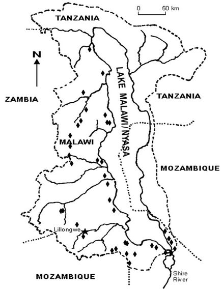
Figure 1. Lake malawi/nyasa basin (Source: [7]).
fish kills and the demise of other aquatic organisms [10, 11]. Although fish kills are a rare occurrence in Lake Malawi, a massive fish kill took place from late September to November in 1999 [12,13]. It was suggested that the upwelling triggered by prolonged southeast trade winds (i.e., Mwera winds) over the lake during the stated period led to the extrusion of hydrogen sulfide from the anoxic hypolimnion zone to the epilimnion, in the process killing a wide spectrum of fish species occupying different ecological niches. Bootsma and Jorgensen [13] further suggested that toxic algae may have been one of the causes of the fish kill. Phytoplankton density in inland water bodies is sometimes used as a measure of anthropogenic disturbance in their watersheds [14,15]: the more degraded the catchment area, the higher the phytoplankton density.
The seasonal fluctuation of primary productivity in Lake Malawi is controlled principally by the thermal structure of the lake, which modulates the mixing of deep water rich in nutrients with that of the phytoplankton rich near-surface layer [16]. The thermal structure in turn is highly dependent on the distribution of solar radiation within the water body. As such, the ability to determine the spatial and temporal distribution of temperature over the lake surface offers an opportunity to obtain vital information about the nature and extent of the existing thermal structure, and also aids in locating upwelling zones in the lake where primary productivity might be taking place. Upwelling zones are generally characterized by the prevalence of cool waters and are normally associated with abundant phytoplankton.
2. Methodology
In order to delineate potential fishing grounds in Lake Malawi, we developed maps showing the spatial and temporal distribution of chlorophyll-a concentration obtained by Moderate-resolution Imaging Spectroradiometer (MODIS/AQUA) and overlaid them on LST maps developed from Advanced Very High Resolution Radiometer (AVHRR) and MODIS/Terra data. Areas with high chlorophyll-a concentration and generally low lake surface temperatures (cool waters) were considered ideal for the development of the fishery industry because of their association with high primary productivity. Details of the methodology for developing chlorophyll and LST maps are outlined in [1,2].
2.1. Distribution of Chlorophyll-a Concentration
Two major activities were carried out in order to develop maps showing the temporal and spatial distribution of chlorophyll-a concentration in Lake Malawi using data from MODIS/AQUA satellite imagery. First, we conducted in situ measurements of chlorophyll concentration at three selected sampling stations over the southeastern arm of Lake Malawi (Figure 2) concurrent with satellite image acquisitions. Second, we downloaded Ocean Color (MODIS/AQUA) Data corresponding with the period of field sampling and used SeaWIFS Data Analysis System (SeaDAS) software [17,18] to determine chlorophyll concentration.
Water samples were collected from the surface of the lake at three stations shown in Figure 2 (Station 1: 14.08˚S, 34.96˚E; Station 2: 14.08˚S, 34.94˚E; and Station 3: 14.07˚S, 34.93˚E). A GPS unit was used to locate the sampling stations. Water sampling was done on clear days over the period May 03 to November 30, 2006. Two liters of water were collected in 20-liter collapsible plastic bottles and kept in a cooler box to avoid exposure to light. The water samples were then transported to a laboratory at Monkey Bay Fisheries Research Station, where the water was filtered on 47 mm GF/F filters under low to moderate vacuum (i.e., less than 8 PSI) to concentrate chlorophyll-containing organisms. Later the concentration of chlorophyll-a concentration in the water was measured.
We also downloaded Level 2 and Level 3 Ocean Color (MODIS/AQUA) Data concurrent with field sampling. From the SeaWIFS Data Analysis System (SeaDAS) main menu, we selected four options, namely: chlorophyll, i.e. an option that intrinsically computes chlorophyll concentration from MODIS imagery using the ratio
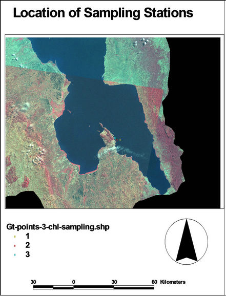
Figure 2. Sampling stations for chlorophyll-a concentration and lake surface temperature.
of normalized reflectance values for bands 10 and 12, or R490/R551; and normalized reflectance data for MODIS/ AQUA bands 9 (R443), 10 (R488), and 12 (R551). We then used equations described in [1] to compute corresponding chlorophyll concentrations. Computed chlorophyll estimates were then compared with in situ data. The Smigen routine of SeaDAS was used for MODIS Ocean Color Level 3 data.
2.2. Distribution of Lake Surface Temperature
Two major tasks were carried out to develop an algorithm to estimate lake surface temperature from satellite imagery. First, we conducted in situ measurements of lake surface temperature at three selected sampling stations over Lake Malawi (Figure 2) at a depth of 0 - 7.0 cm (i.e., skin temperature) concurrent with satellite image acquisitions. The second activity involved downloading and processing AVHRR and MODIS/Terra satellite imagery. AVHRR data covered the period September 1997 to February 1998, whereas MODIS/Terra data covered the period May to November, 2006. For MODIS data, both MODIS Land Surface Temperature (MOD- 11A1) and Ocean Color Sea Surface Temperature (SST) were downloaded from EOS Gateway website and processed into lake surface temperature.
AVHRR data for the period 1997-1998 concurrent with the time when Bootsma and others collected in situ measurements on Lake Malawi at a sampling station located at 13˚30''S and 34˚44.07''E were downloaded from NOAA website. The data then were “sub-setted” for the Lake Malawi Basin (i.e., area of interest, AOI), and digital number (DN) values for bands 3, 4, and 5 were converted to radiance values using the equation described in [2].
For MODIS/Terra (MOD11A1) Land Surface Temperature data, the intrinsic split window equation described in [2] was applied to compute values of LST from bands 31 and 32 using ERDAS Imagine. The procedure entailed downloading MOD11A1 daily (day) temperature data at 1 km resolution, determining the count corresponding with the sampling point and then converting it to temperature in Kelvin by multiplying the count value by a scale factor of 0.02. Thereafter, regression analysis between in situ and MOD11A1 data was conducted, and the value of the r2 was assessed. Contouring of lake surface temperature was done using ER Mapper software with a view to determining the circulation pattern of Lake Malawi.
For MODIS SST, Level 3 temperature data captured by MODIS/Terra satellite were downloaded from the Ocean Color website and processed into lake surface temperature using the Smigen routine in SeaDAS software. The satellite data had a re-sampled resolution of 2 km. Regression analysis between in situ and MODIS SST data was conducted, and the value of r2 was assessed.
3. Results
3.1. Distribution of Chlorophyll-a Concentration
Values of chlorophyll concentration determined from approaches described in [1] using MODIS/AQUA data ranged from 0.35 - 1.83 μg/L while observed values varied from 0.08 - 0.17 μg/L. Generally, the relationship between in situ and computed concentrations of chlorophyll is weak. A plot of the ratio of normalized reflectance at 443 and 551 nm obtained from SeaDAS against observed chlorophyll concentrations gave an r2 value of 0.6 [1]. Figure 3 shows an example of a map of chlorophyll-a concentration distribution over Lake Malawi for May 19, 2005 by applying the equation derived from the regression analysis of in situ chlorophyll-a concentration and the reflectance ratio Rs443/Rs551 using SeaDAS software.
The results show that chlorophyll concentration in the lake is generally low, and varied from 0.05 - 0.27 µg/L. These findings lie within the expected range of annual in situ chlorophyll concentrations in the lake which has a mean value of 1.0 µg/L.
3.2. Distribution of Lake Surface Temperature
Lake surface temperature results obtained from AVHRR using equations described in [16,19] did not closely match in situ data. However, a qualitative assessment of the variation of temperature distribution using ERDAS Imagine with band 4 data of AVHRR for five sampling days yielded temperature maps shown in Figure 4, where the red color represents high temperature, while low temperatures are shown in blue [2].
Temperature distribution maps generally suggest that the lake becomes cool between May and October. This may be attributed to the prevalence of strong Mwera winds (i.e. southeast trade winds) that blow over Lake Malawi during this period, causing upwelling of cold water from the bottom of the lake. But it should also be noted that Malawi experiences cool weather from December to July. Temperature maps further suggest that the location of cold water zones in the lake is not fixed but rather changes with season.
Figure 5 shows a graph of observed lake surface temperature plotted against Land Surface Temperature (i.e., MOD11A1) for Station 1 (Figure 2). The r2 value of 0.7 suggests a relatively strong linear relationship between satellite data and in situ LST. Satellite derived lake surface temperature varied from 22˚C to 25.9˚C.
Presented in Figures 6 and 7 are LST maps derived from MOD11A1 imagery using ER Mapper. In general, it may be said that the lake becomes cool from May to November, a situation very similar to the one depicted by AVHRR satellite imagery (Figure 4). The satellite images also show that the location of upwelling zones in the lake is not static but changes seasonally. However, in the case of MODIS data there is a persistent cold water zone extending from Salima to the north of Nkhotakota. Generally, upwelling zones are fully developed in November, with cold water centers located in the northern tip as wells as the middle section of the lake.
A plot of LST values derived from MODIS SST against observed temperature yielded r2 value of 0.75 (Figure 8), a value slightly higher than that obtained for Land Surface Temperature (i.e. 0.7).
Presented in Figure 9 is the lake surface temperature distribution map developed from the regression equation
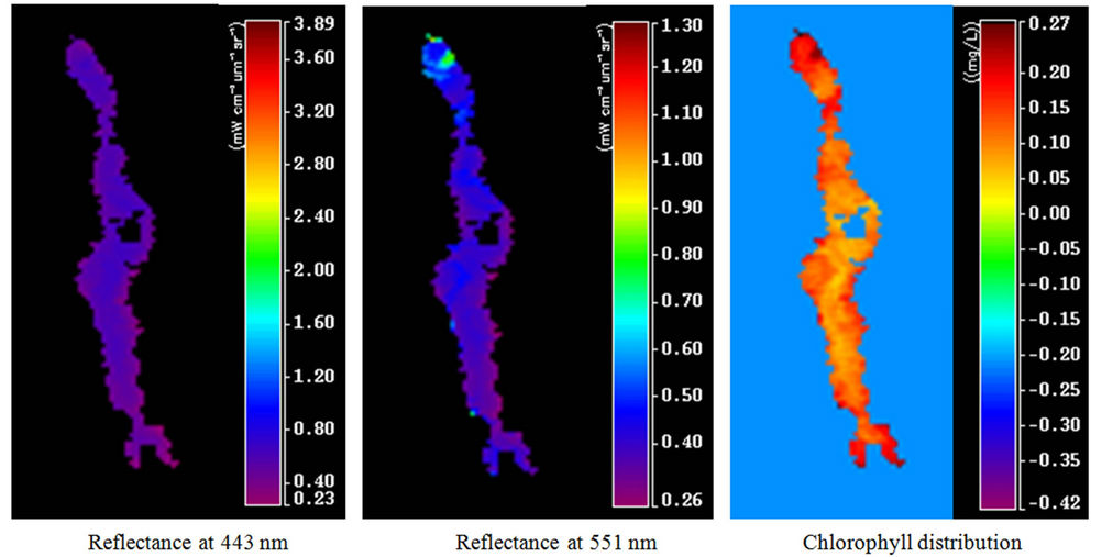
Figure 3. Chlorophyll distribution map, developed from reflectance ratio Rs443/Rs551.
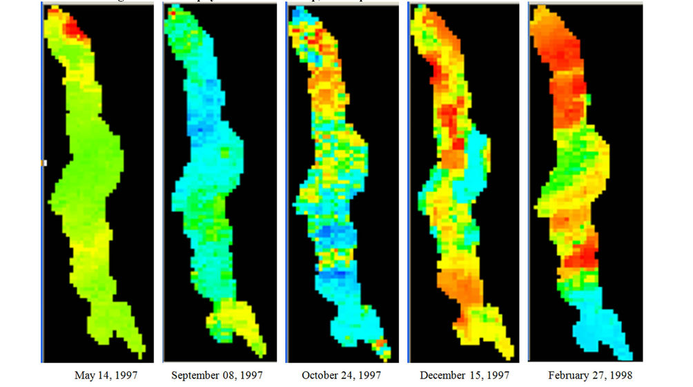
Figure 4. Temperature distribution over Lake Malawi using AVHRR imagery.
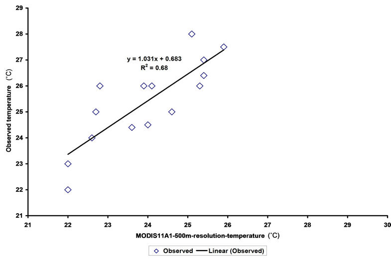
Figure 5. Graph showing MODIS land surface temperature (MOD11A1) plotted against observed LST.
by making use of routines available in SeaDAS.
3.3. Delineating Potential Fishing Grounds
In order to delineate potential fishing grounds in Lake Malawi, we overlaid chlorophyll-a maps with LST maps to demarcate areas of high primary productivity. Figure 10 shows two zones we identified as having great potential for the development of the fishery industry, mainly because of the persistence of cool surface water zones. However, further studies are required to confirm this suggestion with in situ data in terms of the abundance of fish resources in the two delineated areas.

Figure 6. Temperature distribution maps for Lake Malawi, MOD11A1 imagery.
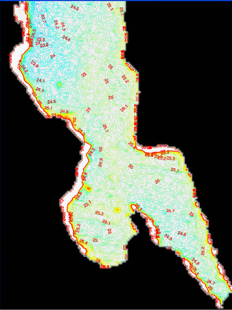
Figure 7. Enlarged LST map for October 03, 2006 (MOD- 11A1), ˚C.
4. Conclusion
This paper has demonstrated how remotely sensed data from MODIS and AVHRR may be used in mapping potential fishing grounds in Lake Malawi. Based on chlorophyll and lake surface temperature data, two areas have been identified where the potential for the development of the fishery industry is high, namely: the zone extending from Salima up to the northern part of Nkhotakota and the northeastern tip of the lake. These areas show characteristics for high primary productivity as evidenced by the prevalence of upwelling cool water from the bottom of the lake and relatively abundant phytoplankton. However, there is need to confirm this suggestion with observed data in terms of the abundance of fish resources in the delineated areas.
5. Acknowledgements
The authors thank the International Water Management Institute (IWMI), University of Minnesota, and START for providing funding for the study. Use of the facilities of the Remote Sensing Laboratory and Water Resources Center at the University of Minnesota and Monkey Bay Fisheries Research Station in Malawi is greatly appreciated. We are happy to acknowledge technical support from James Kuyper, NASA; John Sapper, NOAA; Ye Myint, Leica; Prasad Thenkabail, USGS; and the Ministry
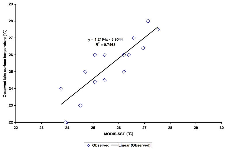
Figure 8. Graph showing MODIS Sea Surface Temperature (SST) plotted against observed Lake Surface Temperature (LST).
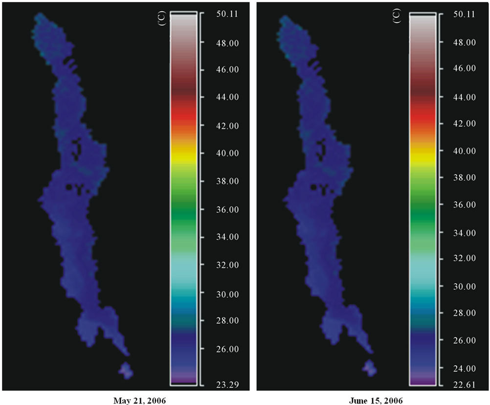
Figure 9. Temperature distribution map for Lake Malawi (˚C), Ocean Color (SST) data.
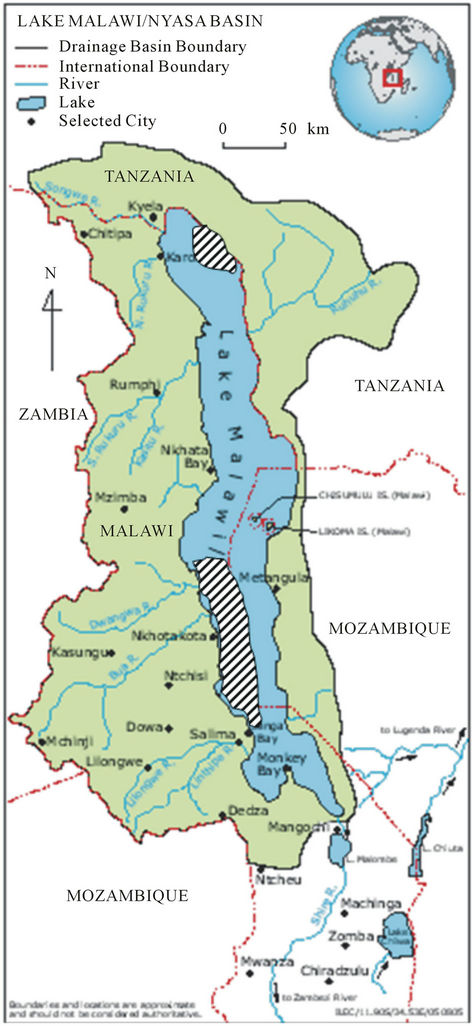
Figure 10. Potential fishing grounds (shaded areas).
of Irrigation and Water Development in Malawi.
REFERENCES
- G. Chavula, P. Brezonik, P. Thenkabail, T. Jonson and M. Bauer, “Estimating Chlorophyll Concentration in Lake Malawi from MODIS Satellite Imagery,” Journal of Physics and Chemistry of the Earth, Vol. 34, No. 13-16, 2009, pp. 755-760.
- G. Chavula, P. Brezonik, P. Thenkabail, T. Jonson and M. Bauer, “Estimating the Surface Temperature of Lake Malawi Using AVHRR and MODIS Satellite Imagery,” Journal of Physics and Chemistry of the Earth, Vol. 34, No. 13-16, 2009, pp. 749-754.
- S. J. R. Bland and S. J. Donda, “Common Property and Poverty: Fisheries Co-Management in Malawi,” Fisheries Bulletin, No. 30, 1995, pp. 1-16.
- G. Patterson and O. Kachinjika, “Limnology and Phytoplankton Ecology,” In: A. Menz, Ed., The Fishery Potential and Productivity of the pelagic zone of the Lake Malawi/Niassa, Natural Resources Institute, London, 1995.
- H. A. Bootsma and R. E. Hecky, Eds., “Water Quality Report,” Lake Malawi/Nyasa Biodiversity Conservation Project, SADC/GEF, 1999.
- S. J. Guildford, R. E. Hecky, W. D. Taylor, R. Mugidde and H. A. Bootsma, “Nutrient Enrichment Experiments in Tropical Great Lakes Malawi/Nyasa and Victoria,” Journal of Great Lakes Research, Vol. 29, Suppl. 2, 2003, pp. 89-106. doi:10.1016/S0380-1330(03)70541-3
- H. A. Bootsma and S. E. Jorgensen, “Lake Malawi/ Nyasa: Experience and Lessons Learned Brief,” 2006. http://www.ilec.or.jp/lbmi2/reports/16_Lake_Malawi_Nyasa_27February2006.pdf
- S. Sathyendranath, G. Cota, V. Stuart, H. Maass and T. Platt, “Remote Sensing of Phytoplankton Pigments: A Comparison of Empirical and Theoretical Approaches,” International Journal of Remote Sensing, Vol. 22, No. 2- 3, 2001, pp. 249-273.
- C. M. Hu, F. E. K. Muller, C. J. Taylor, K. L. Carder, C. Kelble, E. Johns and C. A. Heil, “Red Tide Detection and Tracing Using MODIS Fluorescence Data: A Regional Example in SW Florida Coastal Waters,” Remote Sensing of Environment, Vol. 97, No. 3, 2005, pp. 311-321. doi:10.1016/j.rse.2005.05.013
- S. C. Liew, I. Lin, L. K. Kwoh, M. Holmes, S. Teo, K. Gin and H. Lim, “Spectral Reflectance Signatures of Case 2 Waters: Potential for Tropical Algal Bloom Monitoring Using Satellite Ocean Color Sensors,” 10th JSPS/VCC Joint Seminar on Marine and Fisheries Sciences, Melaka, 29 November-1 December 1999.
- S. Koponen, J. Pullianen, K. Kallio, J. Vepsalainen, T. Pyhalahti, P. Korpinen, M. Kiirikki, J. Koponen and M. Hallikainen, “Use of MODIS Satellite Sensor for Remote Sensing of Phytoplankton Blooms and Turbidity in the Baltic Sea,” International Journal of Remote Sensing, 2012, in Press.
- Ministry of Natural Resources and Environmental Affairs, “Malawi-Lake Malawi Ecosystem,” Project Proposal, GEF, Ministry of Natural Resources and Environmental Affairs, 2002.
- H. Bootsma and S. E. Jorgensen, “Lake Malawi/Nyasa,” In: M. Nakamura, Ed., Managing Lake Basins, Practical Approaches for Sustainable Use, 2004, 36 p. http://www.worldlakes.org/uploads/ELLB%20Malawi-NyasaDraftFinal.14Nov2004.pdf
- A. Genin, B. Lazar and S. Brenner, “Vertical Mixing and Coral Death in the Red Sea Following the Eruption of Mount Pinatubo,” Nature, Vol. 377, No. 6549, 1995, pp. 507-510. doi:10.1038/377507a0
- D. Iluz, Y. Yacobi and A. Gitelson, “Adaptation of an Algorithm for Chlorophyll-a Estimation by Optical Data in the Oligotrophic Gulf of EIlat,” International Journal of Remote Sensing, Vol. 24, No. 5, 2003, pp. 1157-1163. doi:10.1080/0143116021000044797
- M. Wooster, G. Patterson, R. Loftie and C. Sear, “Derivation and Validation of the Seasonal Thermal Structure of Lake Malawi Using Multi-Satellite AVHRR Observations,” International Journal of Remote Sensing, Vol. 22, No. 15, 2001, pp. 2953-2972.
- J. E. O’Reilly, S. Maritorena, B. G. Mitchell, D. A. Siegel, K. L. Carder, S. A. Garver, M. Kahru and C. McClain, “Ocean Color Chlorophyll Algorithms for SeaWIFS,” Journal of Geophysical Research, Vol. 103, No. 11, 1998, pp. 24937-24953. doi:10.1029/98JC02160
- S. B. Hooker and E. R. Firestone, Eds., “SeaWIFS Postlaunch Calibration and Validation Analyses,” NASA Tech. Memo 1999-2068929, Part 1, NASA Goddard Space Flight Centre, Greenbelt, 2000.
- P. S. Thenkabail, “Global Monthly 0.1 Degree (~10 km) AVHRR NDVI Datasets for 1981-2001,” International Water Management Institute (IWMI), Colombo Sri Lanka, 2003.
NOTES
*Corresponding author.