Journal of Applied Mathematics and Physics
Vol.07 No.01(2019), Article ID:90240,10 pages
10.4236/jamp.2019.71019
Existence of Solutions for Boundary Value Problems of Conformable Fractional Differential Equations
Xingyue Jian
College of Science, University of Shanghai for Science and Technology, Shanghai, China

Copyright © 2019 by author(s) and Scientific Research Publishing Inc.
This work is licensed under the Creative Commons Attribution International License (CC BY 4.0).
http://creativecommons.org/licenses/by/4.0/


Received: January 7, 2019; Accepted: January 26, 2019; Published: January 29, 2019
ABSTRACT
In this paper, we study a class of boundary value problems for conformable fractional differential equations under a new definition. Firstly, by using the monotone iterative technique and the method of coupled upper and lower solution, the sufficient condition for the existence of the boundary value problem is obtained, and the range of the solution is determined. Then the existence and uniqueness of the solution are proved by the proof by contradiction. Finally, a concrete example is given to illustrate the wide applicability of our main results.
Keywords:
Boundary Value Problems, Conformable Fractional Differential Equations, The Method of Coupled Upper and Lower Solution, Coupled Solution, Monotone Iteration

1. Introduction
In recent years, there are few studies on boundary value problems of conformable fractional differential equations under new definitions [1] [2] [3] . And conformable fractional derivatives not only have good operational properties (Four Operational Rules of Derivatives, Chain Rule and Leibniz Rule), this definition can also construct fractional Newton equation and Euler-Lagrange equation from fractional variational method, this is of great significance to the study of uniform or uniformly accelerated motion of particles and to the solution of Newton’s fractional-order mechanical problems [4] [5] (fractional-order harmonic oscillator, fractional-order damped oscillator and forced oscillator). And the method of upper and lower solution for monotone iteration can not only gives the existence theorem, but also determines the value range of the solution. Therefore, this method has gradually become an important method for studying nonlinear differential equations [6] [7] [8] [9] . In addition, with the application of anti-periodic boundary value problems in various mathematical models and physical processes has been widely applied, the integral boundaries are also widely used in heat conduction, chemical engineering, groundwater flow, thermoelasticity, plasma physics and other fields. As a result, more and more studies have been made on this kind of problems [10] [11] [12] (anti-periodic boundary value problems, anti-periodic boundary value problems with integral boundaries). However, the indefinite sign of solutions of nonlinear differential equations determines that some problems (anti-periodic boundary value problems and their generalizations) cannot be studied directly by the method of upper and lower solutions for monotone iteration. But the development of nonlinear analysis theory provides a powerful tool for the study of these problems. In the generalized monotone iteration process, the method of coupled upper and lower solution becomes an important method to study this kind of problem by the flexible construction of the comparison theorem [13] [14] [15] [16] . Motivated by the above work, in this paper, the existence of solutions for a class of boundary value problems of conformable fractional differential equations under a new definition is proved by using the method of coupled upper and lower solution, and the range of solutions is obtained. Throughout this paper, we consider the existence of solutions of boundary value problems for the following uniform fractional differential equations
(1)
where is the conformable fractional derivatives of order for which is defined in [1] , and , , , , is continuous.
2. Preliminaries
In this section, we present some definitions and lemmas which will be used in the proof of our main results.
Definition 2.1. (See [1] ) Given a function . Then the conformable fractional derivative of x of order is defined by
for all , . If the conformable fractional derivative of x of order exists, then we simply say that x is δ-differentiable. If x is δ-differentiable in some , , and exists, then we define
Definition 2.2. Let , then are said to be coupled lower and upper solutions of (1), respectively, if
Definition 2.3. Let , then the function pair is said to be coupled solutions of (1), if
Let , then is said to be minimum and maximum coupled solutions of (1), if are coupled solutions of (1), and for any coupled solution .
Lemma 2.1. (See [1] ) Let , and assume to be δ-differentiable, then
1) ;
2) ;
3) .
for , .
Lemma 2.2. (See [1] ) If x is differentiable, , then .
Lemma. 2.3 (See [3] ) If exists, then for , we have .
Lemma 2.4. Assume that , and , , , Define function as follows:
(2)
Then is the solution of the initial value problem as follows
Proof Assume that is given by (2), then p is differentiable for , therefore we have
from Lemma 2.2, and subject to the condition
Lemma 2.5. (Comparison Theorem) Let , and the following inequalities hold true
then , for .
Proof Let , then we have for , and we can draw a conclusion from (2.1) and Lemma 2.3.
3. Conclusions
Theorem 3.1. Assume that are coupled lower and upper solutions of (1.1) with for , let . And if , then the following inequalities hold true
(3)
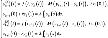
for and . If we take as initial elements, the iterative sequences defined by
(4)
are and , then
1) and uniformly and ;
2) are coupled minimal and maximal solutions of (1.1) respectively in D;
3) If is the solution of (1.1) in D, then we have ; i.e., we have
for .
Proof 1). There is a unique solution to the boundary value problem as follows
which is given by
for and from Lemma 2.2 and Lemma 2.3. Where , . Define operator
where operators are given by
respectively. Then the fixed point of operator T in means the coupled solutions of (1).
Let .
Here we prove that , and are coupled lower and upper solutions of (1).
Whereas
(5)
And are coupled lower and upper solutions of (1), then we have
for . And by Lemma 2.5, we have
So we can easily get that
from formula (3) and (5). i.e., are coupled lower and upper solutions of (1).
We also get that
from formula (5) and . Similarly, we have . by Lemma 2.5.
Let , then from formula (4), we have that are coupled lower and upper solutions of (1) for any , which is similar to the proof above. And
In summary, we have
for . Therefore, function sequences are uniformly bounded, i.e.,
for and . Because f is continuous, we have
for and . In addition, because that functions and are continuous, we have
if and . Hence, is equicontinuous, we can also get that is equicontinuous similarly.
In summary, by Ascoli-Arzela theorem [17] , we can prove that  are convergent because of the monotonicity of Sequences, i.e., there are two functions
 , such that

and . Next we take limits on both sides of (4), then from Lebesgue Dominated Convergence Theorem, we have

if . i.e.,
  are coupled solutions of (1).
2) Here we prove that  are coupled minimal and maximal solutions of (1) respectively in D.
Assume that  are a set of coupled solutions of (1), then the above problem is equivalent to prove that

Whereas , therefore
 . Assume that
  for
for , here we prove that
 .
.
Consider that
And from Definition 2.3, we have that

Then from (3), we get that

In that way, we have

according to Lemma 2.5. By Mathematical Induction, we can get

for . In addition, because of the convergence of iterative sequences, we have

if . i.e.,

for . Therefore,
  are coupled minimal and maximal solutions of (1) respectively in D from Definition 2.3.
3) Here we prove that if x is the solution of (1) in D, then . In conclusion (2) above, let
 , because that x is the solution of (1) in D, therefore,
  are a set of coupled solutions of (1). Obviously, x subject to

In summary, Theorem 3.1 is proved.
Theorem 3.2. Assume that  is increasing in x on
  , and
, and , then there exists a unique solution of (1) in
 .
.
Proof By Theorem 3.1, we get that  and
and . And we have
  for
for . Then we have that
  for
for . Here we prove that
 .
.
If  is increasing in x on
 , assume that
 , then we have

considering the convergence of iterative sequences. Let , then we have
  by Lemma 2.2, i.e., the function
  is monotonically decreasing. Hence,
  , therefore, we draw a contradiction from the conclusion that
 , which can be obtained from the condition
  and the boundary value conditions above. Therefore, we have
 , i.e.,
  is the solution of (1).
On the basis of (1), we can also consider the existence of solutions of boundary value problems for the following uniform fractional differential equations:
 (6)
(6)
where  is the conformable fractional derivatives of order
  for
for  which is defined in [1] , and
 ,
,  ,
,  ,
,  is continuous. Similarly, the existence of the solution can be proved by the method of coupled upper and lower solution, and the range of the solution can be obtained. Due to
 , so the original problem needs to be solved until the solution of the equation of order n before we construct the comparison theorem, which is the difficulty of (6).
4. Examples
To illustrate our main results, we present the following example.
Example 4.1. Consider the boundary value problem of conformable fractional differential equations under the following new definitions
 (7)
(7)
It is obvious that  are coupled lower and upper solutions of (7), and from the condition
 , we can get that there exists a constant
  for
for , such that the formula (4) of Theorem 3.1 holds. Hence, problem (4) has at least one solution
  for
for  by Theorem 3.2.
Example 4.2. Consider the boundary value problem of conformable fractional differential equations under the following new definitions
 (8)
(8)
where , it is easy to get that

which yield to

Therefore,  are coupled lower and upper solutions of (8), it is obvious that the formula (4) of Theorem 3.1 holds. Hence, problem (8) has at least one solution
  for
for  by Theorem 3.2.
Conflicts of Interest
The author declares no conflicts of interest regarding the publication of this paper.
Cite this paper
Jian, X.Y. (2019) Existence of Solutions for Boundary Value Problems of Conformable Fractional Differential Equations. Journal of Applied Mathematics and Physics, 7, 233-242. https://doi.org/10.4236/jamp.2019.71019
References
- 1. Khalil, R., Al Horani, M., Yousef, A. and Sababheh, M. (2014) A New Definition of Fractional Derivative. Journal of Computational and Applied Mathematics, 264, 65-70.
- 2. Anderson, D.R. and Avery, R.I. (2015) Fractional-Order Boundary Value Problem with Sturm-Liouville Boundary Conditions. Eprint Arxiv, 29.
- 3. Batarfi, H., Losada, J. and Nieto, J.J. (2015) Three-Point Boundary Value Problems for Conformable Fractional Differential Equations. Journal of Function Spaces, 2015, Article ID: 706383.
- 4. Chung, W.S. (2015) Fractional Newton Mechanics with Conformable Fractional Derivative. Journal of Computational and Applied Mathematics, 290, 150-158. https://doi.org/10.1016/j.cam.2015.04.049
- 5. Benkhettou, N., Hassani, S. and Torres, D.F.M. (2015) A Conformable Fractional Calculus on Arbitrary Time Scales. Journal of King Saud University Science, 28, 93-98. https://doi.org/10.1016/j.jksus.2015.05.003
- 6. Wei, Z.L., Dong, W. and Che, J.L. (2010) Periodic Boundary Value Problems for Fractional Differential Equations Involving a Riemann-Liouville Fractional Derivative. Nonlinear Analysis-Theory Methods and Applications, 73, 3232-3238.
- 7. Wei, Z.L. and Dong, W. (2011) Periodic Boundary Value Problems for Riemann-Liouville Sequential Fractional Differential Equations. Electronic Journal of Qualitative Theory of Differential Equations, 87, 1-13. https://doi.org/10.14232/ejqtde.2011.1.87
- 8. Zhang, W., Bai, Z.B. and Sun, S.J. (2016) Extremal Solutions for Some Periodic Fractional Differential Equations. Advances in Difference Equations, 179, 1-8.
- 9. Mu, J. and Li, Y.X. (2012) Periodic Boundary Value Problems for Semilinear Fractional Differential Equations. Mathematical Problems in Engineering, 1-16.
- 10. Xu, Y.F. (2016) Fractional Boundary Value Problems with Integral and Anti-Periodic Boundary Conditions. Bulletin of the Malaysian Mathematical Sciences Society, 39, 571-587.
- 11. Qiao, Y. and Zhou, Z.F. (2017) Existence of Solutions for a Class of Fractional Differential Equations with Integral and Anti-Periodic Boundary Conditions. Qiao and Zhou Boundary Value Problems, 1-9.
- 12. Matar, M.M. (2017) Existence of Integral and Anti-Periodic Boundary Valued Problem of Fractional Order . Bulletin of the Malaysian Mathematical Sciences Society, 40, 959-973.
- 13. Luo, Z.G. and Wang, W.B. (2006) Existence of Solutions for Antiperiodic Boundary Value Problems of Second Order Differential Equations. Journal of Applied Mathematics, 29, 1111-1117.
- 14. Wang, W.B. and Shen, J.H. (2009) Existence of Solutions for Anti-Periodic Boundary Value Problems. Nonlinear Analysis: Theory, Methods and Applications, 70, 598-605.
- 15. Devi, J.V. (2008) Generalized Monotone Method for Periodic Boundary Value Problems of Caputo Fractional Differential Equations. Communications in Applied Analysis, 12.
- 16. Ramrez, J.D. (2014) Generalized Monotone Iterative Method for Caputo Fractional Differential Equations with Anti-Periodic Boundary Conditions. Dynamic Systems and Applications, 23, 479-492.
- 17. Guo, D.J., Sun, J.X. and Liu, Z.L. (2006) Functional Method for Nonlinear Ordinary Differential Equations. Shandong Science and Technology Press.