American Journal of Operations Research
Vol. 2 No. 3 (2012) , Article ID: 22442 , 12 pages DOI:10.4236/ajor.2012.23051
Are Securities Also Derivatives?
Department of Quantitative Finance, National Tsing Hua University, Hsinchu, Taiwan
Email: kpchang@mx.nthu.edu.tw
Received May 21, 2012; revised June 20, 2012; accepted July 8, 2012
Keywords: Arbitrage Theorem; Derivatives; Home-Made Security; Capital Structure Irrelevancy; Share and Mixed Labor Contracts
ABSTRACT
This paper has used the Arbitrage Theorem (Gordan Theorem) to show that first, all securities are derivatives for each other, and they are priced by the same risk neutral probability measure. Second, after the firm changes its debt-equity ratio, the equityholders can always combine the new equity with other existing securities to create a home-made equity which will give exactly the same time-1 payoff of the old equity. That is, we have a capital structure irrelevancy proposition: changes in firms’ debt-equity ratios will not affect equityholders’ wealth (welfare), and equityholders’ preferences toward variance are irrelevant. Third, when the firm moves from a more certain project to a more uncertain one, the time-0 price of equity will increase, but (because the time-1 payoff of common bond has an upper bound) the time-0 price of common bond will decrease. Fourth, different labor contractual arrangements will not affect the time-0 price of labor input. When the firm moves from a more certain project to a more uncertain one, the time-0 price of labor input will increase if it is under the share or the mixed contract.
1. Introduction
The seminal work of Black and Scholes (1973) has inspired many researches on pricing and hedging different financial contracts [1]. The literature argues that options and their underlying assets are different: a rise in the variability of the underlying asset will decrease its market value, but this rise will increase the market value of the option. Some studies also argue that an option value depends only on its underlying asset, and it does not depend on the random prices of other securities or portfolios. I think these arguments are wrong. In this paper, I first derive the Arbitrage Theorem, and then use the theorem to show that all securities are derivatives for each other, and they depend on each other. The paper also derives a capital structure irrelevancy proposition: changes in firms’ debt-equity ratios will not affect equityholders’ wealth (welfare), and equityholders’ preferences toward variance are irrelevant. When the firm moves from a more certain project to a more uncertain one, the time-0 price of equity will increase, but the time-0 price of common bond will decrease. Different labor contractual arrangements will not affect the time-0 price of labor input. When the firm moves from a more certain project to a more uncertain one, the time-0 price of labor input will increase if it is under the share or the mixed contract.
The remainder of this paper is organized as follows. Section 2 derives the Arbitrage Theorem and uses the theorem and several examples to show that securities are derivatives for each other; and that after the firm changes its debt-equity ratio, the equityholders can always combine the new equity with other existing securities to create a home-made equity which will give exactly the same time-1 payoff of the old equity. Concluding remarks appear in Section 3.
2. Arbitrage Theorem and Valuation of Contracts
Theorem 1:
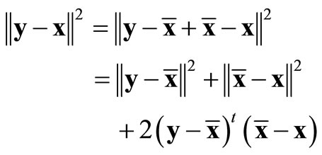
Let S be a nonempty, closed convex set in Rn and . Then, there exists a unique point
  with minimum distance from y. Also,
  is the minimizing point if and only if
  for all
 .
.
Proof We first show the existence of a minimum point. Since S is not empty, there exists a point . Define
 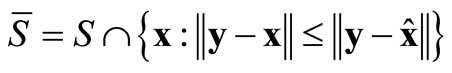 and hence,
 .
.
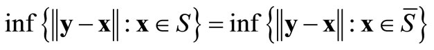
Since 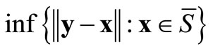 means finding the minimum of a continuous function over a nonempty, compact set
 , by Weierstrass’ theorem, there exists a minimizing point
  in S that is closest to the point y.
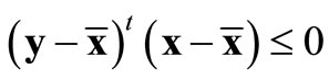
To show the uniqueness of minimum point, suppose that there is another 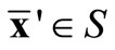 which is also a minimum point, i.e.,
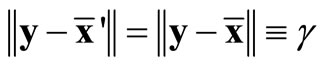 . By convexity of S,
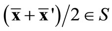 . By Schwartz inequality, we get
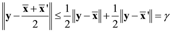
If strict inequality holds, we have a contradiction to  being the closest point to y. Therefore, equality holds, and we must have
 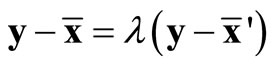 for some λ. Since
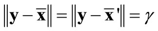 ,
,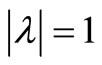 . If λ = –1, then
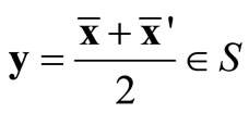
which contradicts the assumption . Thus, λ = 1, and we have
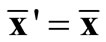 .
.
Suppose  for all
 . Then,
Since 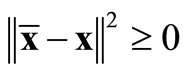 and
and 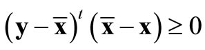 by assumption,
 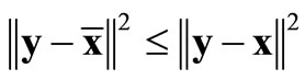 for all
 , i.e.,
  is the minimizing point. Conversely, assume that
  is the minimizing point. Let
  and 0 ≤ α ≤ 1. We have
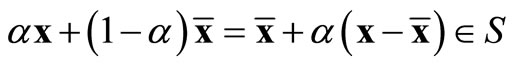
and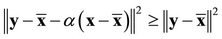 . Therefore, from
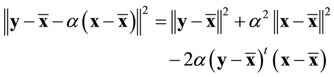
we can get 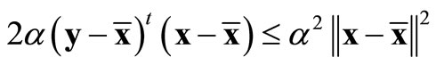 for all 0 ≤ α ≤ 1. Dividing this inequality by any such α > 0
 and letting α → 0+, we have
  for all
 .
. 
Theorem 2 (Separating Hyperplane Theorem):
Let S be a nonempty, closed convex set in Rn and . Then, there exists a nonzero vector
  and a scalar α such that
 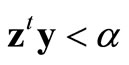 and
and 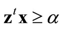 for each
 .
.
Proof From Theorem 1 we know that because the set S is a nonempty, closed convex set in Rn and , there exists a unique minimizing point
  that
that
 for all
 .
.
Letting 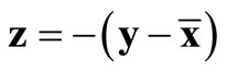 and
and , we have zt(x –
 )≥ 0 and hence,
  for each
 . Also, zty – α = zt(y –
 ) = –(y –
 )t(y –
 ) < 0 or
 .
. 
Theorem 3 (Farkas Theorem):
Let A be an m × n matrix and  be a vector. Then, exactly one of the following systems has a solution:
System 1: Ax ≥ 0 and ctx < 0 for some 
System 2: Aty = c and y ≥ 0 for some 
Proof 1) Suppose that System 2 has a solution; that is, there exists a  and y ≥ 0 such that Aty = c. Then, if for any
  such that Ax ≥ 0, then
 ; that is, System 1 has no solution.
2) Suppose System 2 has no solution. Form the set . Note that the set S is a closed convex set: Let
  and
and . Then there must exist
  such that x1 = Aty1 and x2 = Aty2. Also,
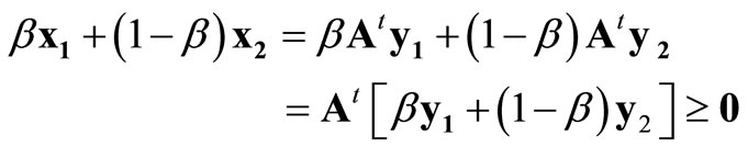
where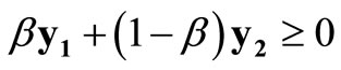 .
.
Since , by Theorem 2, there exists a nonzero vector
  and a scalar α such that ztc < α and
 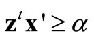 for each
 . Because
 ,
, .
.  for each y ≥ 0. Since y can be made arbitrarily large and α is a fixed number, we must have Az ≥ 0. We have therefore constructed a vector
  such that Az ≥ 0 and ztc < 0, i.e., System 1 has a solution.
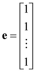
Theorem 4 (Gordan Theorem or Arbitrage Theorem):
Let A be an m × n matrix. Then, exactly one of the following systems has a solution:
System 1: Ax > 0 for some 
System 2: Atp = 0 for some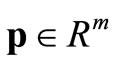 , p ≥ 0, etp = 1 where
 .
.
Proof 1) Suppose that System 1 has a solution: Ax > 0 for some . Then, we can construct a negative scalar δ < 0 and a vector
such that Ax +δe ≥ 0, or 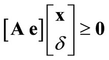 and
and
 .
.
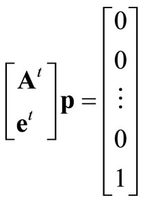
Define ,
,  , and
, and . We have
 ,
,  and
and ; that is, System 1 of Theorem 3 has a solution.
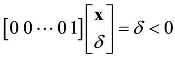
2) With the same definitions, System 2 of Theorem 3 can be interpreted as: There exists a vector p ≥ 0 and  such that
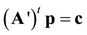 . That is,
 or Atp = 0 and etp = 1 (i.e.,
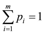 ).
). 
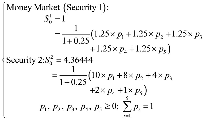
In System 2 of the Arbitrage Theorem, the vector p is usually termed as the risk neutral probability measure, and pi, i = 1, ···, m, can be interpreted as the current price of one dollar received at the end of period if state i occurs. If the matrix A has rank m (i.e., the matrix has m independent rows), the risk neutral probability measure p will be unique. We now use the Arbitrage Theorem to clarify some ambiguous (and erroneous) arguments in the literature.
Example 1. All Securities Are Derivatives.
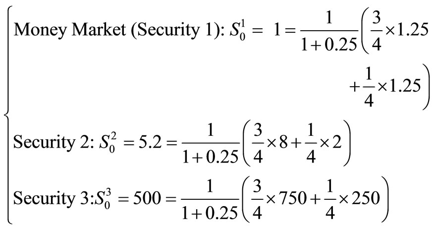
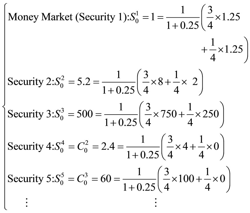
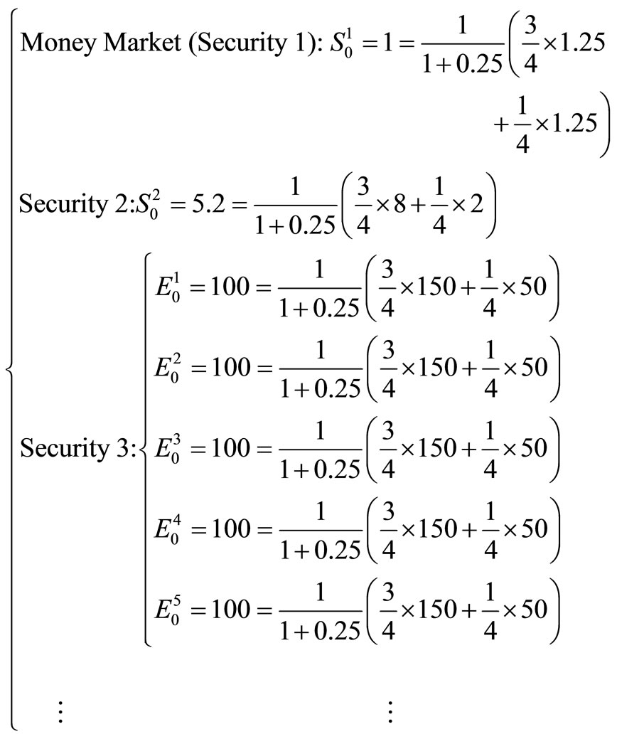
Assume a one-period, two states of nature world with no transaction costs. There are a money market (Security 1) which provides 1 + 0.25 dollars at time one if one dollar is invested at time 0 (i.e., the interest rate is r = 0.25), and two other securities (Security 2 and Security 3) with current prices 4 and 500 dollars, respectively, which provide:
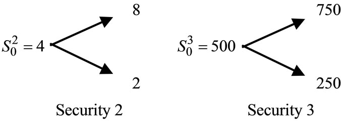
Note that the two securities are not governed by the same risk neutral probability measure (i.e., System 2 of the Arbitrage Theorem has no solution):
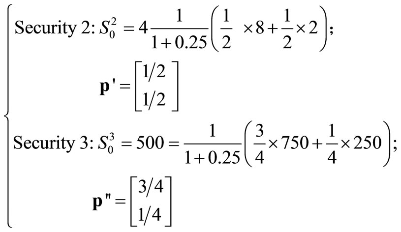
i.e., we cannot find a vector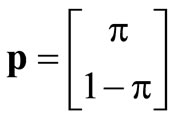 , 0 ≤ π ≤ 1such that
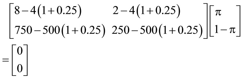
By System 1 of the Arbitrage Theorem, arbitrage exists: e.g., at time 0, we can short sell one share of Security 3, buy 60 shares of Security 2 and invest 260 (= 500 – 4 × 60) dollars in the money market, and at time 1 we can get net profit:
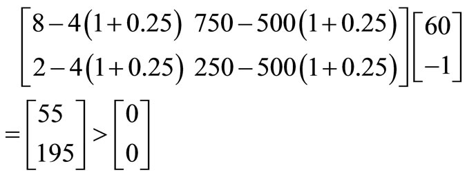
Hence, in equilibrium (with no arbitrage), the time-0 prices of Security 2 and Security 3 will change so that they are priced by the same risk neutral probability messure, say,
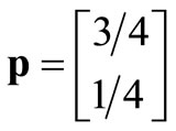 and
and
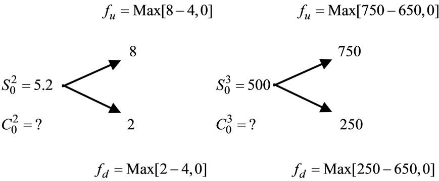
Suppose that two European call options are based on Security 2 (with strike price 4 dollars) and Security 3 (with strike price 650 dollars), respectively:
Since all the securities are governed (priced) by the same, unique risk neutral probability measure
 we will have:
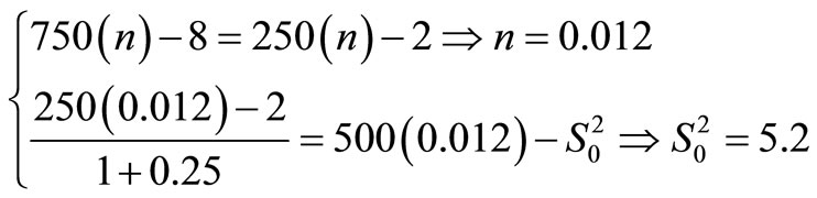
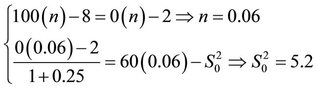
Also, at time 0, by buying n shares of the underlying asset and selling one call to construct a portfolio which gives certain time-1 payoff, the prices of the two European calls can be derived from Security 2 or Security 3:
For :
:
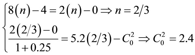
or 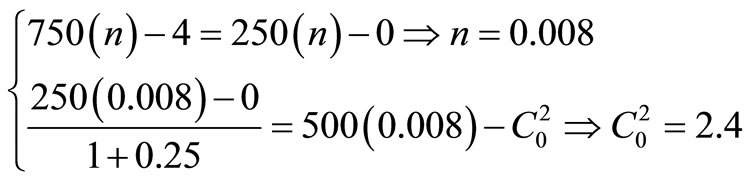
For :
:
or 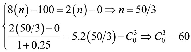
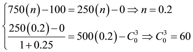
The time-0 price of Security 2 can be derived from Security 3 or the options, and the time-0 price of Security 3 can be derived from Security 2 or the options:
For :
:
or
For :
:
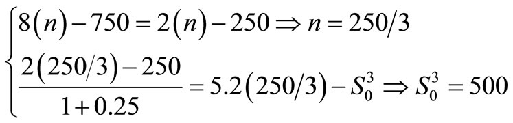
or
Thus, we can conclude that all securities are derivatives for each other, and all securities are underlying assets for each other. This result refutes Cox, Ross and Rubinstein’s (1979) [2] claim that “the only random variable on which the call value depends is the stock itself. In particular, it does not depend on the random prices of other securities or portfolios” (p. 235).1
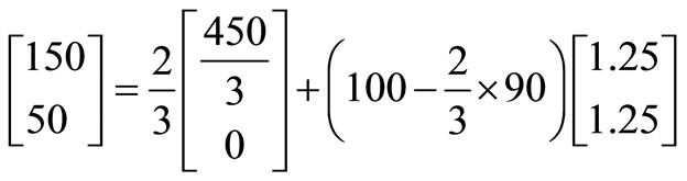
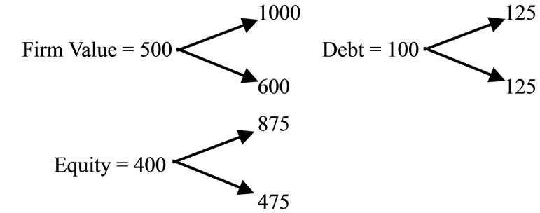
Example 2. Home-made Securities.
In Example 1, assume that Security 3 is a firm and is the sum of five shares of equity:
 (1)
(1)
Suppose that the fourth and the fifth shares of equity ( and
and ) of the firm are changed into riskless debts (
 and
and ):
):
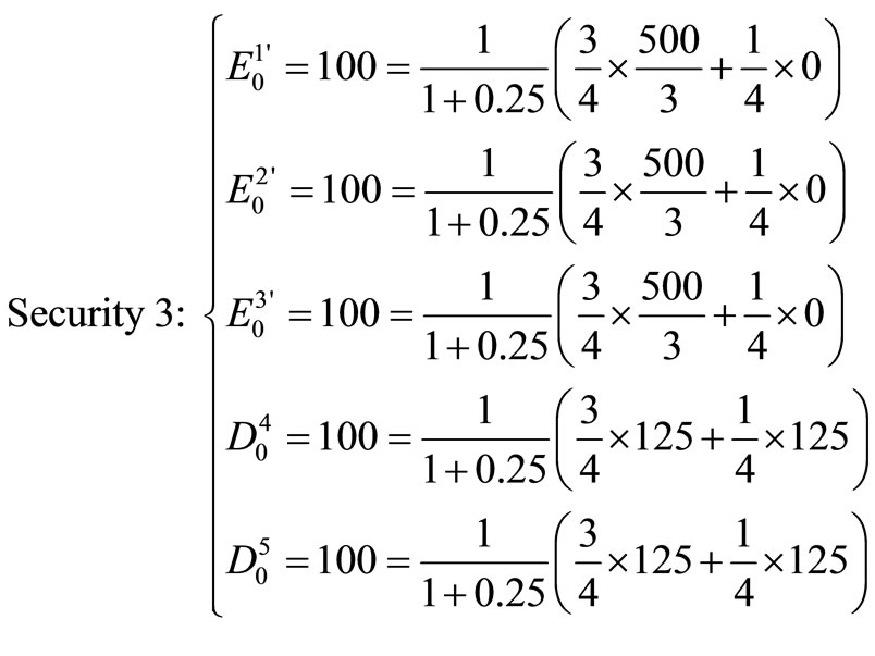 (2)
(2)
The market value of the firm (Security 3) at time 0 is still 500 dollars; that is, the market value of firm is independent of its debt-equity ratio. This is just a restatement of Modigliani-Miller’s first proposition.2
Comparing Equation (1) with Equation (2), it is found that more debt means higher variance of equity’s time-1 payoff:

But after the firm changes its debt-equity ratio, the equityholders can always buy only 0.6 shares of the new equity ( ) and invest 40 (= 100 – 0.6 × 100) dollars in the money market to recreate the time-1 payoff of the old equity (
 ):
):
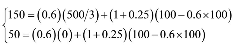
or
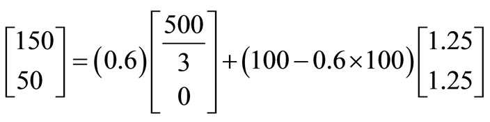 (3)
(3)
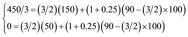
Suppose that in Equation (2), debts are risky:
 (4)
(4)
Again, after the firm changes its debt-equity ratio, the equityholders can always buy 2/3 shares of the new equity ( ) and invest
 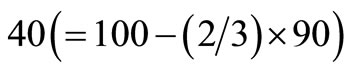 dollars in the money market to recreate the time-1 payoff of the old equity (
 ):
):
 (5)
(5)
That is, after the firm changes its debt-equity ratio, the equityholders can always combine the new equity with other securities (e.g., money market) to create a “home-made equity” which will give exactly the same time-1 payoff of the old equity.3 We now have a capital structure irrelevancy proposition: changes in firms’ debt-equity ratio will not affect equityholders’ wealth (welfare), and equityholders’ preferences toward variance are irrelevant.4 This result refutes the claims in the literature that “the use of debt rather than equity funds to finance a given venture may well increase the expected return to the owners, but only at the cost of increased dispersion of the outcomes” (Modigliani and Miller, 1958 [4], p. 262); “any gains from using more of what might seem to be cheaper debt capital would thus be offset by correspondingly higher cost of the now riskier equity capital” (Miller, 1988, p. 100) [5]; and “the levered stockholders have better returns in good times than do unlevered stockholders but have worse returns in bad times, implying greater risk with leverage” (Ross, Westerfield and Jaffe, 2010 [6], p. 496).5
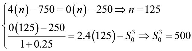
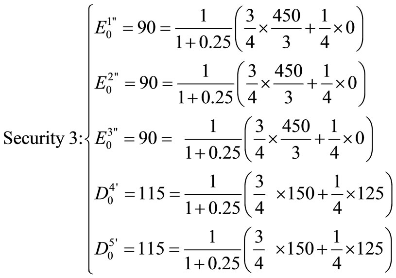
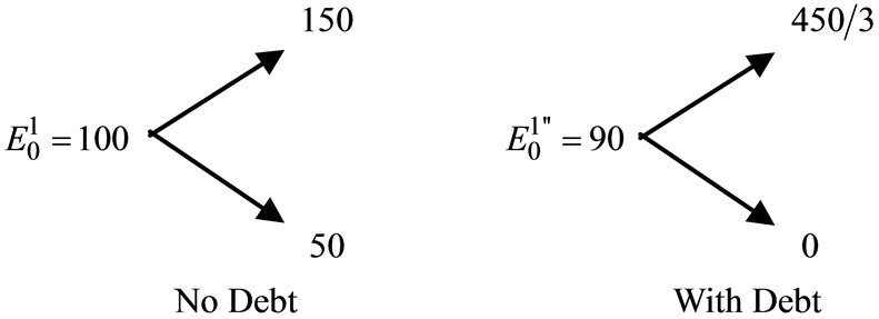
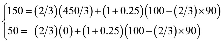
Example 3. Pricing Debt and Equity Contracts.
In Example 2, assume Equation (4) where Security 3 is a levered firm:
 (4’)
(4’)
Suppose that the firm moves to a more uncertain project, and its time-1 payoff is  rather than
 .
.
Then, Equation (4’) becomes:
 (5’)
(5’)
It is found that when the firm moves from a more certain project (its time-1 payoff is either $750 or $250) to a more uncertain one (its time-1 payoff is either $900 or $100), the variance of the time-1 payoff of the firm (and the variance of the time-1 payoff of the equity) increases, the time-0 price of equity increases, but the time-0 price of debt decreases.6 Also, this redistribution effect of wealth between debtholders and equityholders has nothing to do with their attitudes toward risk. These results and the results of Example 1 refute the claims that “there is a fundamental distinction between holding an option on an underlying asset and holding the underlying asset. If investors in the marketplace are risk-averse, a rise in the variability of the stock will decrease its market value” (Ross, Westerfield and Jaffe, 2010 [6], p. 689); and “in most financial settings, risk is a bad thing; you have to be paid to bear it. Investor in risky (high-beta) stocks demand higher expected rates of return. High-risk capital investment projects have correspondingly high costs of capital and have to beat higher hurdle rates to achieve positive NPV. For options it’s the other way around” (Brealey, Myers and Allen, 2006 [7], p. 557).
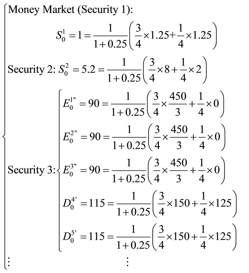
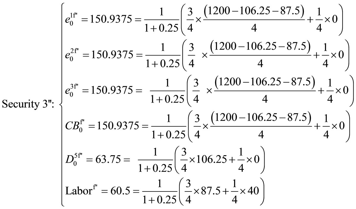
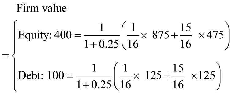
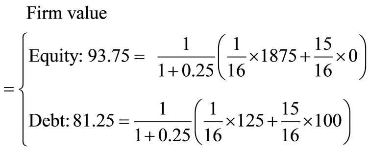
Example 4. Pricing Convertible Bonds.
In Example 2, assume Equation (2) where Security 3 is a levered firm. Assume that one of the firm’s riskless debts is changed into a convertible bond:
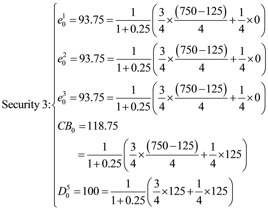 (6)
(6)
Adding this convertible bond dilutes the time-0 value of the equity (which decreases from 100 dollars to 93.75 dollars). The time-0 price of the option (the right) of converting the bond into a share of equity is 18.75 (= 118.75 – 100) dollars.
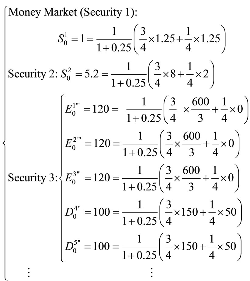
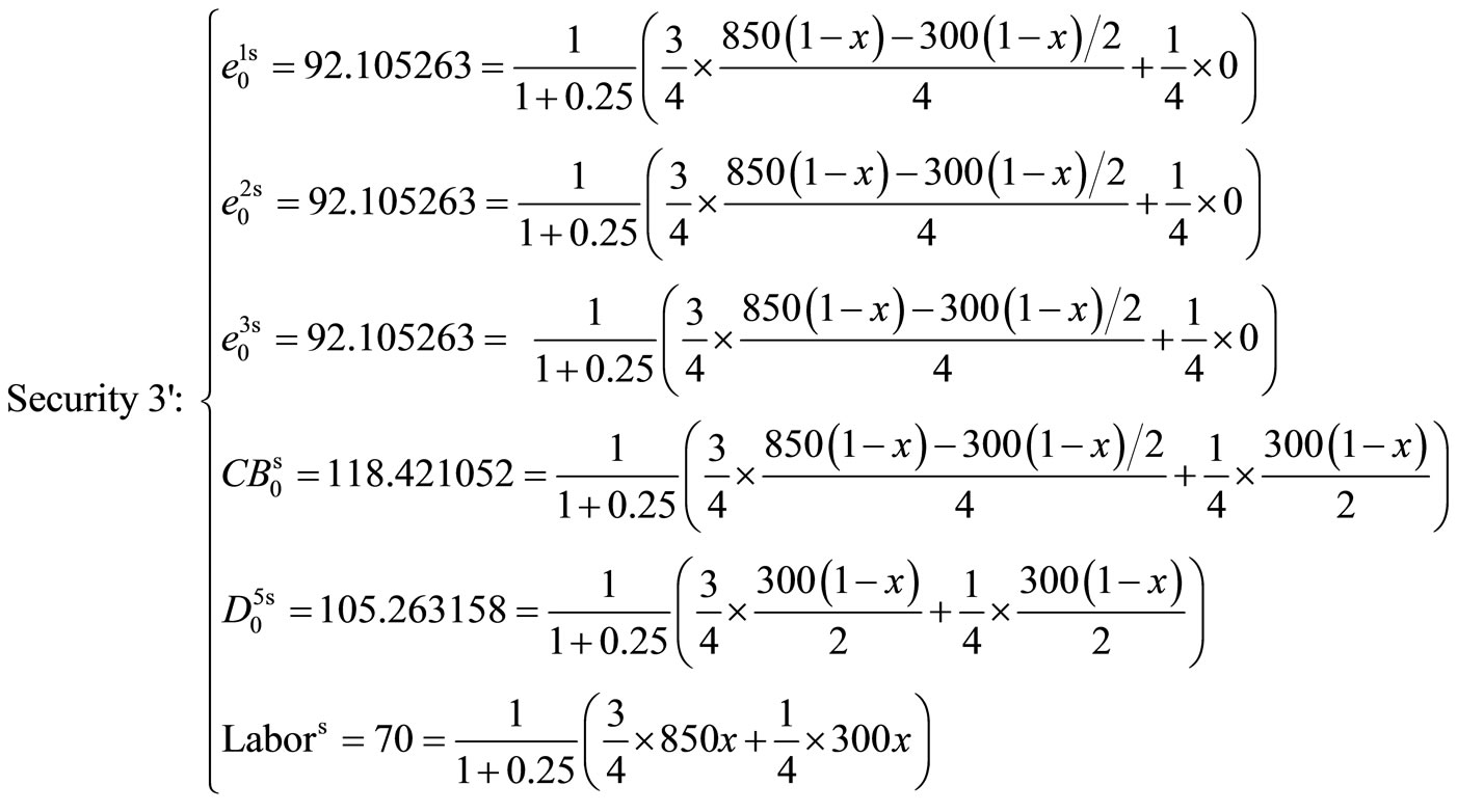
Example 5. Pricing Different Contracts.
In Example 4, assume Equation (6) where Security 3 is a levered firm. Suppose that the firm’s hiring an additional labor (a manager) can increase its time-1 payoff from  to
to :
:
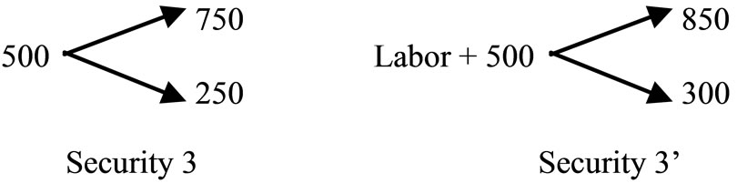
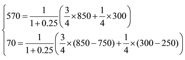
The time-0 value of the whole firm will be 570 dollars, and the time-0 value of the labor input will be 70 dollars:
Note that different labor contractual arrangements will not affect the time-0 prices of the labor input and the whole capital input (which includes equity, debt and convertible bond):7
Fixed-wage contract:
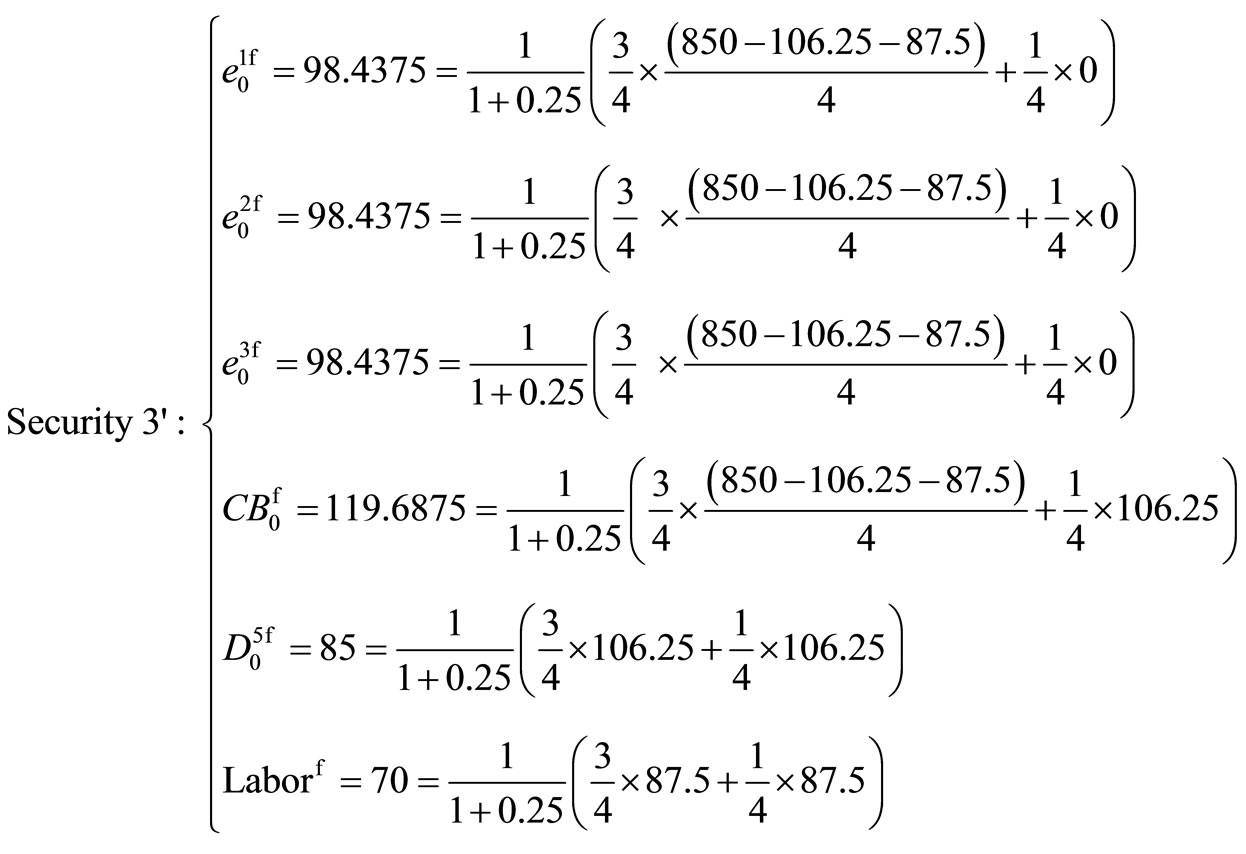 (7)
(7)
Share contract (where the labor’s share: ; the capital providers’ share:
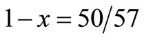 ):
):
 (8)
(8)
Mixed contract (where the labor obtains 50 dollars and has share: , and capital providers’ share is:
 ):
):
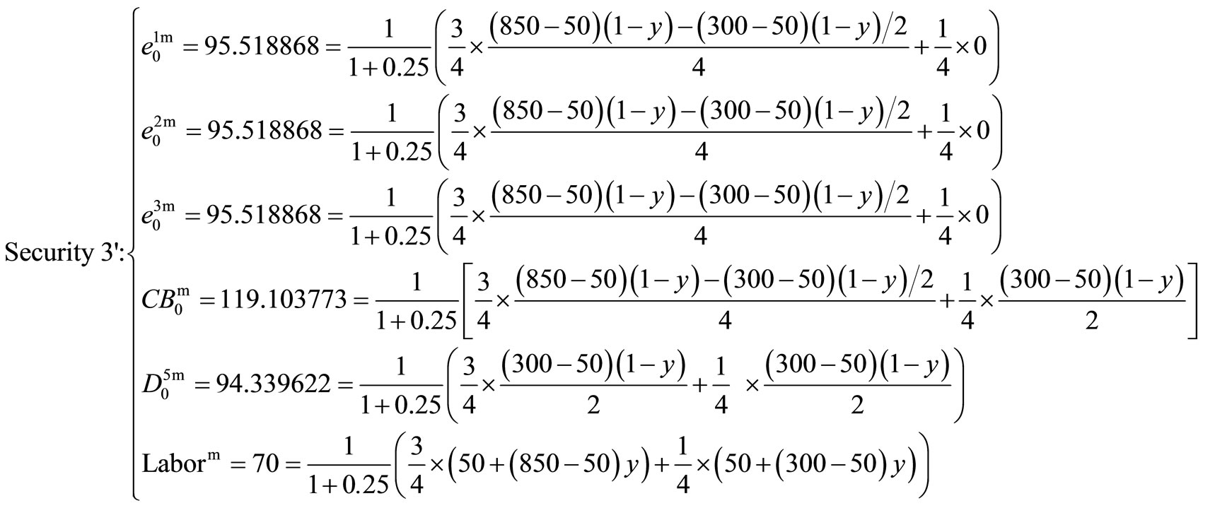 (9)
(9)
Suppose the firm moves to a more uncertain projectand its time-1 payoff is  rather than
 and assume that the labor is the first to get payment, the common bondholder is the second to get payment, the convertible bondholder is the third to get payment, and the equityholder obtains the residual:
Fixed-wage contract:
 (7’)
(7’)
Share contract (where labor share: ; capital providers share:
 ):
):
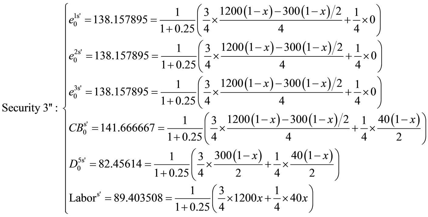 (8’)
(8’)
Mixed contract (where the labor obtains 50 dollars and has share: , and capital providers’ share is:
 ):
):
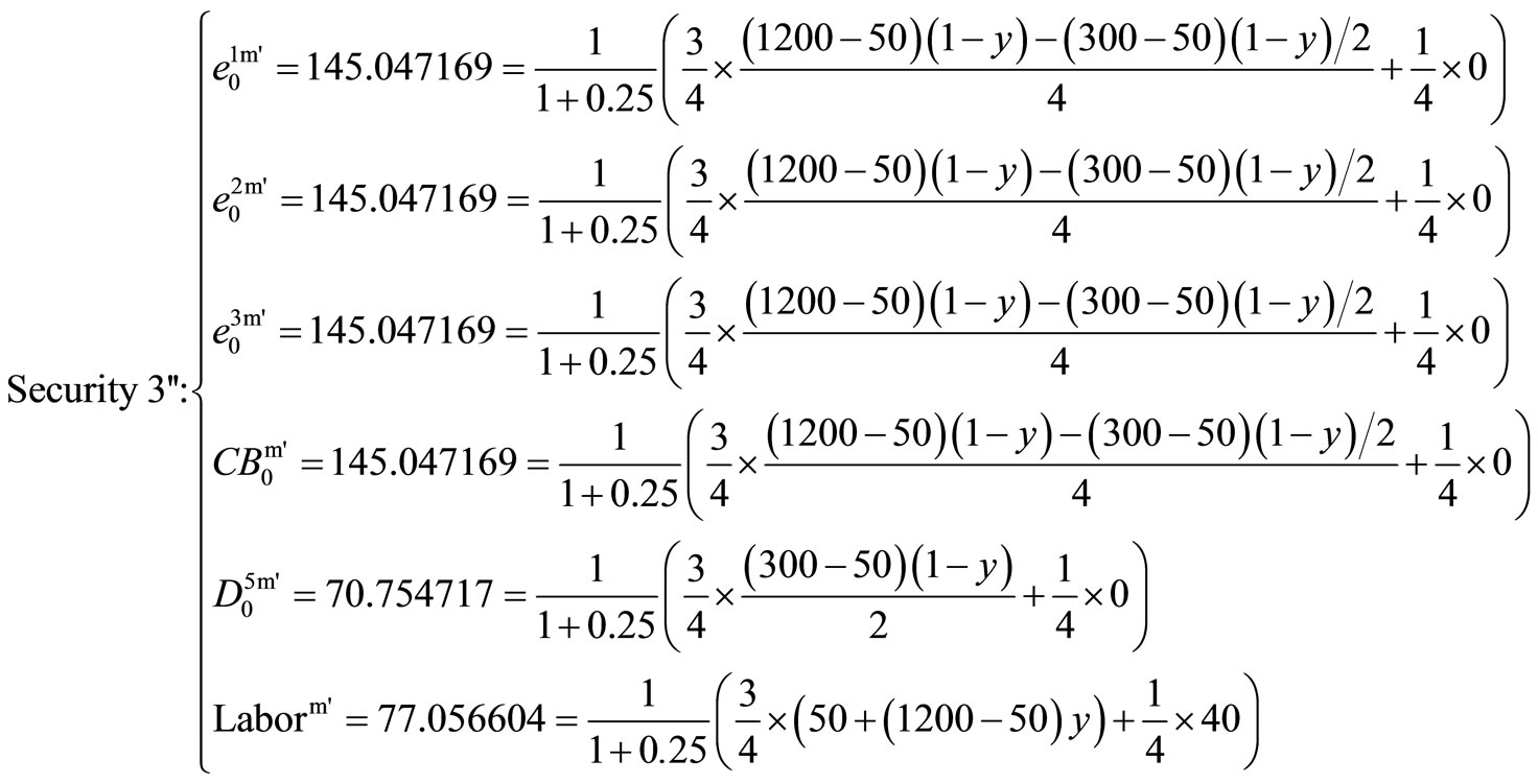 (9’)
(9’)
The time-0 prices of the whole firm, the equity and the convertible bond will increase. The time-0 price of the common bond will decrease. The time-0 price of the labor input will decrease if it is under the fixed-wage contract. The time-0 price of the labor input will increase if it is under the share or the mixed contracts.
3. Concluding Remarks
This paper has used the Arbitrage Theorem (Gordan Theorem) to show that first, all securities are derivatives for each other, and they are priced by the same risk neutral probability measure. Second, after the firm changes its debt-equity ratio, the equityholders can always combine the new equity with other existing securities to create a home-made equity which will give exactly the same time-1 payoff of the old equity. That is, we have a capital structure irrelevancy proposition: changes in firms’ debtequity ratios will not affect equityholders’ wealth (welfare), and equityholders’ preferences toward variance are irrelevant. Third, when the firm moves from a more certain project to a more uncertain one, the time-0 price of equity will increase, but (because the time-1 payoff of common bond has an upper bound) the time-0 price of common bond will decrease. Fourth, different labor contractual arrangements will not affect the time-0 price of labor input. When the firm moves from a more certain project to a more uncertain one, the time-0 price of labor input will increase if it is under the share or the mixed contract.
REFERENCES
- F. Black and M. Scholes, “The Pricing of Options and Corporate Liabilities,” Journal of Political Economy, Vol. 81, No. 3, 1973, pp. 637-654. doi:10.1086/260062
- J. Cox, S. Ross and M. Rubinstein, “Option Pricing: A Simplified Approach,” Journal of Financial Economics, Vol. 7, No. 3, 1979, pp. 229-263. doi:10.1016/0304-405X(79)90015-1
- K. P. Chang, “A Reconsideration of the ModiglianiMiller Propositions,” 2004. http://ssrn.com/abstract=657921
- F. Modigliani and M. Miller, “The Cost of Capital, Corporation Finance and the Theory of Investment,” American Economic Review, Vol. 48, No. 3, 1958, pp. 261-297.
- M. Miller, “The Modigliani-Miller Propositions: After Thirty Years,” Journal of Economic Perspectives, Vol. 2, No. 4, 1988, pp. 99-120. doi:10.1257/jep.2.4.99
- S. Ross, R. Westerfield and J. Jaffe, “Corporate Finance,” McGraw-Hill, New York, 2010.
- R. Brealey, S. Myers and F. Allen, “Principles of Corporate Finance,” McGraw-Hill, New York, 2006.
- S. Cheung, “Private Property Rights and Sharecropping,” Journal of Political Economy, Vol. 76, No. 6, 1968, pp. 1107-1122. doi:10.1086/259477
- R. Litzenberger and H. Sosin, “The Theory of Recapitalizations and the Evidence of Dual Purpose Funds,” Journal of Finance, Vol. 32, No. 5, 1977, pp. 1433-1455. doi:10.1111/j.1540-6261.1977.tb03346.x
- C. Huang and R. Litzenberger, “Foundations for Financial Economics,” Elsevier Science Publishing, New York, 1988.
Appendix A
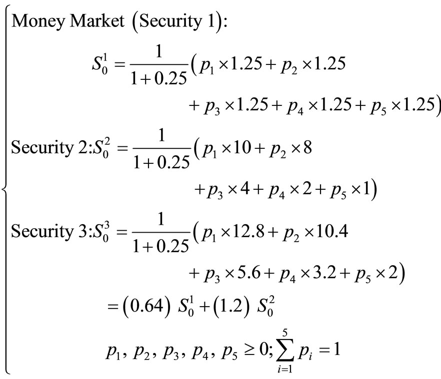
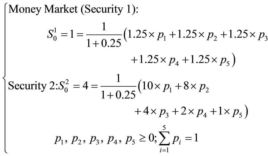
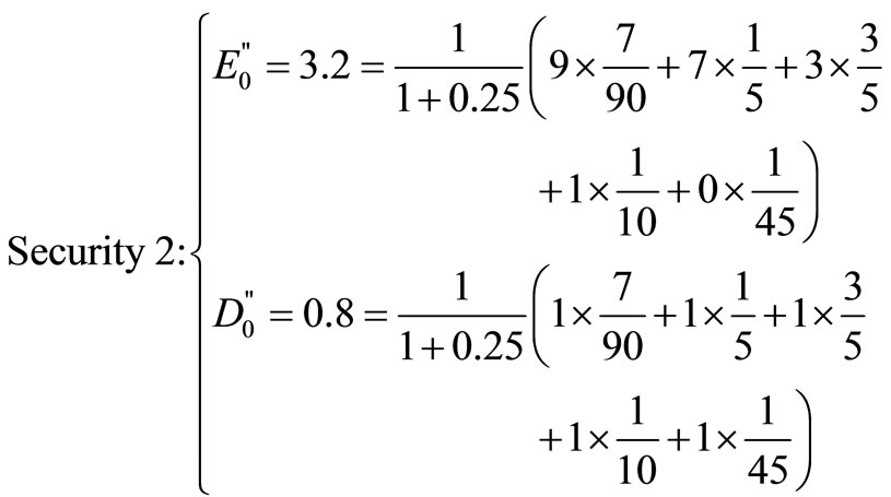
In incomplete markets, securities may not be derivatives for each other, but with no arbitrage (System 2 of Theorem 4 has a solution), they will still be priced by the same (which may not be unique) risk neutral probability measure. For example, assume that only two securities (one of them is a money market with interest rate r = 0.25) exist in a no-arbitrage, one-period, five states of nature world:
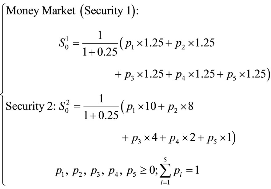
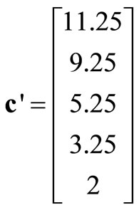
Suppose that there is a new security: Security 3 whose time-1 payoff is: 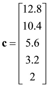 .
.
Because c lies in the subspace spanned by
 and
and 
(i.e.,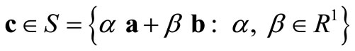 ), the time-1 payoff of Security 3 can be derived (replicated) by those of Securities 1 and 2:
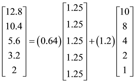
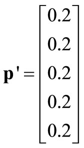
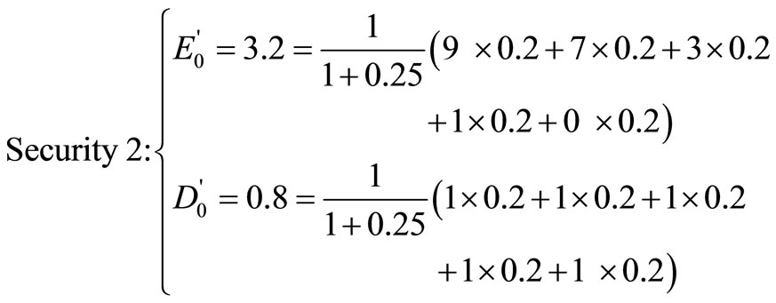
The time-0 price of Security 3 is: 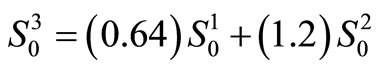 , and with no arbitrage, the three securities are priced by the same risk probability measure:
Suppose that the time-1 payoff of Security 3 is:
 .
.
Because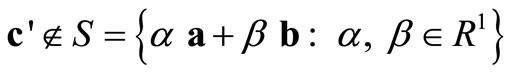 , the time-1 payoff of Security 3 cannot be replicated by those of Securities 1 and 2. But with no arbitrage (System 2 of Theorem 4 has a solution), all the three securities will be priced by the same risk probability measure:
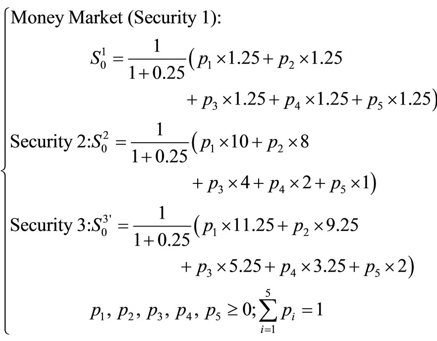
where p1, p2, p3, p4, p5 may not be unique.
Appendix B
In incomplete markets, after the firm changes its debtequity ratio, the equityholders may not be able to create a home-made equity to replicate the time-1 payoff of the old equity. For example, assume that only two securities (one of them is a money market with interest rate r = 0.25) exist in a no-arbitrage, one-period, five states of nature world:
 (B1)
(B1)
where the risk neutral probability can be
 or
or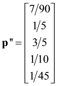 .
.
Assume that Security 2 is an all equity firm and it plans to issue a riskless debt (debtholder pays 0.8 dollar at time 0, and obtains 1 dollar at time 1):
By ,
,
or, by ,
,
That is, recapitalization through issuing riskless debt does not change the market value of the firm (i.e., the time-0 price of Security 2 is always 4 dollars), and the time-0 prices of equity and debt are independent of the risk neutral probability measure used. Also, after the firm issues riskless debt, the equityholder can always create a home-made equity by combining the new equity ( or
or ) with investing 0.8 dollar in the money market, which will give exactly the same time-1 payoff of the old equity:
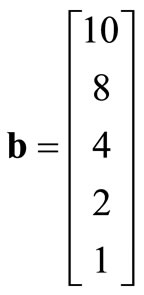 .
.
Suppose that the time-1 payoff of the debt is uncertain:
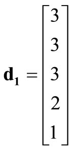 and the time-1 payoff of the equity is:
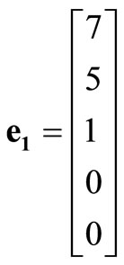 .
.
Since 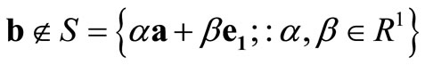 where
where
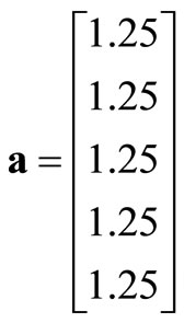 and
and b cannot be replicated by a and e1. That is, the equityholder cannot combine the new equity e1 with the money market to create a home-made equity to replicate the time-1 payoff of the old equity:
 .
.
Also, with different risk neutral probability measures:
By ,
,
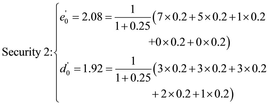
By ,
,
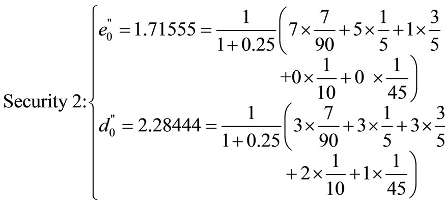
The time-0 price of Security 2 can be the sum of  and
and  (which is equal to 4.36444 > 4), and with no arbitrage,

where the risk neutral probability can be
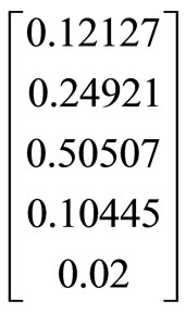 or
or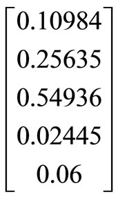 .
.
If this is the case, then with no arbitrage, the time-0 price of Security 2 in Equation (B1) will be adjusted to 4.36444 dollars in the first place (see also Litzenberger and Sosin, 1977 [9]; and Huang and Litzenberger, 1988 [10], pp. 128-129):
 (B1’)
(B1’)
where p1, p2, p3, p4, p5 may not be unique.
Appendix C
In some cases, the time-0 price of a firm may decrease when the firm moves to a more uncertain project. For example, assume a firm exists in a no-arbitrage, oneperiod, two states of nature world (where the market interest rate is: r = 0.25):
That is, the unique risk neutral probability for this world is:
 and
and
 (C1)
(C1)
Suppose the firm moves to a more uncertain project, and its time-1 payoff is

instead of  .
.
Then, the time-0 prices of the whole firm, the equity and the debt decrease:
 (C2)
(C2)
Since no one (especially, the equityholder) benefits, the firm will not move to this more uncertain project, and Equation (C2) does not exist.
NOTES
1This example and the following examples assume complete markets; i.e., the matrix A of System 2 of Theorem 4 has m independent rows. In incomplete markets, securities may not be derivatives for each other, but with no arbitrage (i.e., System 2 of Theorem 4 has a solution), they will still be priced by the same (which may not be unique) risk neutral probability measure. See Appendix A.
2For a simpler proof of this proposition without using any math, see Chang (2004) [3].
3Note that even before the firm changes its debt-equity ratio, the equityholders can buy 3/2 shares of the existing equity ( ) and borrow 60 (
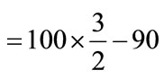 ) dollars from the money market to create the time-1 payoffs of the new equity (
 ):
): .
.
4After the firm changes its debt-equity ratio, the debtholders can also combine the new debt with other securities to create a home-made debt which will give exactly the same time-1 payoff of the old debt (i.e., debtholders’ preferences toward variance are irrelevant). Thus, in complete markets, mean-variance analysis may not be meaningful.
5In incomplete markets, after the firm changes its debt-equity ratio, the equityholders may not be able to create a home-made equity to replicate the time-1 payoff of the old equity. See Appendix B.
6Because the debtholders’ time-1 payoff has an upper bound, they will not benefit if the more uncertain project succeeds, and they will suffer if the more uncertain project fails. Note that in some cases, the time-0 price of a firm may decrease when the firm moves to a more uncertain project. See Appendix C.
7With the assumption of certainty, Cheung (1968) [8] finds that different labor contractual arrangements will not affect the efficiency of resource allocation.