Open Journal of Marine Science, 2012, 2, 70-83
http://dx.doi.org/10.4236/ojms.2012.22010 Published Online April 2012 (http://www.SciRP.org/journal/ojms)
Model for Predicting the Transport and Dispersal of
Contaminants Incoming with Submarine
Groundwater: Case Study for the Southwestern
Taiwan Coastal Zone
Konstantin A. Korotenko1, Peter O. Zavialov1, Ruey-Chy Kao2, Chung-Feng Ding2
1Shirshov Institute of Oceanology, Russian Academy of Sciences, Moscow, Russia
2Tainan Hydraulics Laboratory, National Cheng-Kung University, Tainan, Chinese Taipei
Received February 29, 2012; revised March 19, 2012; accepted March 26, 2012
ABSTRACT
As was recognized recently, the submarine groundwater transports a significant amount of various contaminants into
the coastal ocean. An assessment of the impact of intruded pollutants in the coastal ecosystems requires understanding
fate of the pollutants and processes of their dispersal in ambient waters. In this paper, we proposed a 3-D coupled ocean
circulation/particle-tracking model for predicting the transport and dispersal of pollution-containing groundwater dis-
charged into a coastal environment of the southwestern Taiwan. The particle-tracking model takes currents and turbu-
lent diffusivities predetermined by the ocean circulation model and uses the Lagrangian approach to predict the motion
of individual droplets, the sum of which constitutes a contaminant plume in result of discharge of contaminant-rich
submarine groundwater. The ocean circulation model was forced by tides and seasonal favorable winds for the south-
western coast of Taiwan. The initialization of the coupled model was set using field data obtained in 2009 on the Ping-
tung shelf where shallow aquifer seepages were discovered. Several types of numerical experiment scenarios were set
up to elucidate the transport and dispersal of conservative and nonconservative (nitrate) contaminants in the shallow
coastal zone. The comparison of obtained numerical results with observations performed by other researches was dis-
cussed.
Keywords: Submarine Groundwater; Coastal Zone; Nitrate; Eulerian-Lagrangian Model; Taiwan
1. Introduction
Submarine groundwater discharge (hereinafter SGD) has
been recognized as the potentially significant contribu-
tion to the coastal ocean [1]. Although not as obvious as
river discharge, groundwaters (hereinafter SGs) can also
discharge directly into the coastal ocean. Like surface
water, groundwater flows downgradient. Therefore, ground-
water flows directly into the coastal ocean wherever a
coastal aquifer is connected to the sea. Furthermore, arte-
sian aquifers can extend for considerable distances from
shore, underneath the continental shelf with discharge to
the coastal ocean at their points of outcrop. In some cases,
these deeper aquifers may have fractures or other breaches
in the overlying confining layers, allowing groundwater
to flow into the sea Figure 1(b) schematically illustrates
shallow and deep aquifers and processes associates with
SGD.
Very importantly, it is now recognized that groundwa-
ter discharge may be an important pathway for diffuse
pollution to enter the coastal zone where coastal aquifers
have become contaminated by septic systems or other
pollution sources [2]. Despite SGD contribution in the
ocean’s water budget is generally small, it represents an
important source of nutrients and other contaminants that
affect the ecology of the estuaries and coastal fresh water
bodies [1,3-7]. There are reports that SGD may also be
an important source of alkalinity and carbon to shelf wa-
ters [8].
Submarine groundwater coming from coastal aquifers
into the coastal ocean carries dissolved contaminants,
concentration and type of which considerably varied from
region to region. Multiple studies indicate that the con-
centration of groundwater contaminants increases with
increasing housing density and agriculture activity. Ex-
panding residential and commercial near-shore develop-
ment is leading to increased nutrient inputs to groundwa-
ter that eventually migrate into to coastal waters. Several-
decades long research shows that nitrogen inputs via
C
opyright © 2012 SciRes. OJMS

K. A. KOROTENKO ET AL. 71
Figure 1. Map of the Pingtung coastal zone showing the bathy metry off southwestern Taiw an and stations of hydrographical
observations (marked by solid circles) in the area of the shallow SG well (marked by the solid square). The lower inset (2b)
epicts the schematic (no scale) of processes associated with SGD (after [1]). d

K. A. KOROTENKO ET AL.
72
non-point sources over large coastline areas cause de-
cline of ecological health and may support harmful algal
blooms [9].
In Taiwan, investigations of the offshore discharge of
groundwater, for many years, were largely motivated by
water resource related issues. As was noted by [10], there
were at least two reasons why scientific studies have de-
veloped so slowly in this field. First, the SGD process is
inherently very difficult to measure and monitor, which
tended to discourage serious investigations. Nearshore
seepages around Taiwan typically have very diffuse and
highly variable unit fluxes although the cumulative dis-
charge can be very significant when it occurs over a wide
area. Second, SGD is a process that occurs across a land-
sea interface that spans different scientific disciplines as
well as environments. Unfortunately, there are distinct
cultural and structural differences that separate terrestrial
and marine scientists. Literally, hydrologists and coastal
oceanographers are looking at the same problem from
different ends.
For the last decade, intensive field investigations of
coastal environment pollution associated with SGD are
undertaken in coastal zone of Taiwan including its south-
western part (Figure 1). In [11], it was found out that
aquifers are significant sources of trace elements and
other chemical constituents to the southwestern coastal
waters of Taiwan where onland chemicals as NH4, SO4,
NO3, PO4 and SiO2, hydrocarbons, trace metals (Ni, Cu,
Cd), NaOH, fertilizers, and sewage were. Reference [11]
also reported the exploratory discovery of SGD by using
salinity in Taiwan for the first time in the coastal area
and point out that SGD may occur near the Kaoping
River estuary. Recently [12,13] have shown that subma-
rine groundwaters are also clearly indicated by tracers of
oxygen, strontium isotopes and barium content. They
noted that the concentration of many contaminants in
groundwater is typically several times higher than in
seawater. Usually with distance from seepage the con-
centration of contaminants decreased rapidly. As obser-
vations of nitrate (NO3) plumes near shallow seepages by
[7,14] shows, the flux of nitrate towards the marine en-
vironment was highly variable even over a short distance
from the coast. In addition, greater dispersion near the
seepage face due to movement of water masses in re-
sponse of tides and to seasonal cycles of recharge to the
fresh aquifer. Outside an aquifer, nitrate diminished sub-
stantially in concentration so that horizontal and vertical
sizes of a detectable inclined nitrate plume did not ex-
ceed 6 and 4 m, respectively [7].
In the coastal ocean, processes of spreading and fate of
contaminants coming from SG aquifers are governed by
ocean dynamics and depend on many factors as seepage
zone, discharge rate and type of contaminants. Mathe-
matically, predicting such processes is very a compli-
cated task that requires developing numerical models for
reproducing/predicting the ocean circulation and trans-
port of contaminants. Until now, numerical modeling
directed to the solution of problems associated with pol-
lution inputs from SGD is mostly focused on modeling
the transport and biogeochemical processes [9,15,16]
inside aquifers. Some works have been dedicated to ana-
lysis and modeling an influence of tides on oscillation of
groundwater discharge rate [2,17,18]. By theoretical mo-
del for SGD and the associated chemical transfer to the
ocean, [2] have demonstrated that wave setup and tidal
pumping may be the processes largely responsible for the
high rate of SDG and, in turn, a considerable intensifica-
tion of the transport of chemicals to the ocean. Despite
wide spectra of models and approaches that were built
for the solution of various problems associated with con-
tamination of coastal zone due to SDGs, yet, no attempt
has been made on the development of a complex ap-
proach for predicting the regional circulation and its ef-
fect on the transport and mixing of pollutants coming
into seawater from submarine seepages. Therefore the
objective of this work is to fill this gap and develop a
pollution transport model coupled with an ocean circula-
tion model. In the work, we will focus on the shelf zone
of the southwestern Taiwan, however, based on the gen-
eralized approach, the model can be adapted easily for
any region of interest.
The paper is structured as follows: In Section 2, a short
description of region of interest, hydrology and charac-
teristics of SG based on field observations are given. In
Section 3, the coupled circulation/particle-tracking model
is introduced. In Section 4, results numerical experiments
with conservative and nonconservative (nitrate) tracers
under wind and tidal forcings as well as discussion are
presented. Summary is given in Section 5.
2. Study Region
Figure 1 shows the coastal zone of the southwestern
Taiwan. The marine environment in this area is rather
unique in terms of geomorphology. A major feature the
latter is Gaoping (submarine) Canyon, belonging to the
river extension type canyon, and Siaoliuciou Island. The
canyon is well aligned with the Gaoping River on land,
runs across the continental shelf, continues its course
southwestward onto the continental slope, and terminates
at a depth of about 3000 m. The head of the canyon, cut-
ting the continental shelf, is characterized by high and
steep walls, and the cross-sectional morphology of the
canyon varies from V-shaped to broadly U-shaped [19].
As field observations exhibited [19,20], such peculiari-
ties in geomorphology have a great effect on coastal cir-
culation and mixing processes.
Complex hydrographic study of submarine groundwa-

K. A. KOROTENKO ET AL. 73
ter discharge in the Pingtung coastal zone [12,13] al-
lowed finding seepage locations by tracing oxygen, stron-
tium isotopes. Areas with notable SGD1 were found to
locate a long distance from the shoreline (~25 km) and
likely to be widespread off southwestern Taiwan.
To detect shallow SGDs, quantify their rate and influ-
ence on the local hydrology as well as define the content
of contaminants, the joint oceanographic observations
were conducted by Taiwanese and the Russian scientific
groups in February and October 2009 on the Pingtung
shelf [21]. Figure 1 schematically depicts the transec-
tions of the polygon where hydrophysical and hydro-
chemical observations have been conducted. The solid
circles depicted along the transections denote location of
hydrographical stations conducted during both expedi-
tions.
Distinct manifestations of submarine groundwater dis-
charge were revealed near-shore, west of the Siaoliuciou
Island at stations 11 and 16 (Figure 1). In the vicinity of
the SG seepage (marked by solid squared in Figure 1),
CTD measurements revealed salinity inversions on pro-
files in the 2 m bottom layer (Figure 2(b)), where the
magnitude of the salinity drop reached 0.06 psu. For such
salinity drop, the SGD rate, as was estimated by [21],
should be in range between 0.1 and 1 gm–2·s–1. The esti-
mation was based on the advection-diffusion balance of
salinity in the water column affected groundwater inflow,
dd
z
wSK Sz, where S is salinity, z is vertical coordi-
nate, w is mean vertical velocity of groundwater seepage
and Kz is the eddy diffusivity.
Assuming that salinity difference, , in the bottom
inverse layer,
S
H

w
, significantly less than mean salinity
in the bottom ambient water, S0, i.e., 0, we ob-
tain the velocity and SGD rate per
unit area,
SS

1

1
0z
wKSS H



Q

, where

is mean density. Taking
average values S0 = 30 psu, Kz = 10–4 m
2·s–1 and

=
1025 kg·m–3, for = 0.06 and S
H
 = 2 m, we obtain
w = 0.864 cm·day–1 and Q = 1.025 g·m–2·s–1.
The deviation of vertical velocity and magnitude of the
SGD rate, obtained by [21], is associated with variations
of and
S
H
 estimated from field experiments. Be-
sides uncertainties in estimation of and
S
H
 the rate,
Q, depends on vertical diffusivity, Kz, which was chosen
from general assumptions. Actually, Kz can significantly
vary in the bottom boundary layer and thus the estimates
of w and Q can be considered as an order of magnitudes.
Nevertheless they agree with the characteristic values
reported earlier for well-developed SGD at other loca-
tions in the ocean [22].
The field observations also revealed that the salinity
inversions coincided with maxima of dissolved oxygen,
organic matter content, iron and phosphorus concentra-
tions, and the minimum of turbidity. Note that, in non-
impacted by SGD areas, ambient waters were character-
ized by regular salinity profiles with the maximum of
salinity at the bottom (Figure 2(a)).
Many studies show that SGD makes a significant con-
tribution to nutrient budget of coastal water that causes
significant research interest in this phenomenon [6,12,18].
We made chemical analyses of water samples collected
from the bottom layer of the ocean, as well as the near-
shore land groundwater well (marked by solid square in
Figure 1) and Kaoping River in February 2009. The re-
sults for nitrate, NO3, which we focus on, are depicted in
Table 1.
As seen, measurements conducted at stations 1, 6, 11,
16 and near the SG well revealed that nitrate concentra-
tions were higher than those at other stations not affected
by SGD. This difference in NO3 concentrations appears
to be consistent with the figures reported by [8] for the
same area. Note that the increasing concentrations of
NO3 observed at stations #11 and #16 cannot be ex-
plained by the river inputs, because the nitrate content in
Kaoping River water was considerably lower. Above the
SG well, the nitrate concentration reached 0.48 mg·L–1
that significantly exceeded that in seawater.
Current velocity measurements conducted near by the
SG well (Figure 1) indicated that along- and cross-shore
components of the velocity exhibited a superposition of
about 0.1 m·s–1 amplitude of the tidal and background
northwestward coastal current of about 0.25 m·s–1.
3. Coupled Model Description
Modeling the transport and dispersal of contaminant-
containing fresh groundwater from a coastal aquifer into
(a) (b)
Figure 2. Typical temperature, T, and salinity, S, profiles
obtained in the 5-m layer (a) far from the seepage (at station
15) and (b) those obtained near the seepage (after [21]).
1Note that SGD can be submerged springs or point sources and often
are diffuse across large areas in the ocean.

K. A. KOROTENKO ET AL.
74
Table 1. Chemical indicators of the water samples collected
from the bottom layer of the ocean, groundwater well, and
Kaoping River in February, 2009. Bold values indicate SGD
impacted seawater (after [21]).
Station # Distance, km Nitrate, mg·L–1
1 0.5 0.04
2 1.7 0.03
5 1.9 0.04
6 0.4 0.04
7 6.8 0.02
8 5.0 0.02
9 2.9 0.02
10 1.2 0.02
11 0.3 0.03
12 6.9 0.02
13 5.0 -
14 3.0 0.01
15 1,3 0.01
16 0.4 0.02
Average N/A 0.02
Average sites N/A 0.03
GW Well N/A 0.48
Kaoping River N/A 0.06
the adjacent shallow marine environment presents a real
challenge to oceanographers. Difficulties are associated
with many factors such as the hydrostatic instability of
bottom fresh water discharging into the saline environ-
ment, uncertainties of the SGD rate estimate, seepage
location(s) as well as with difficulties of predicting coa-
stal currents induced by variable forcing (wind, tides,
etc.). All these factors are necessary to take into account
in deciding on the choice of a particular numerical model
and approach. Our approach to the solution of the trans-
port and dispersal of contaminant-containing fresh ground-
water is based on the Lagrangian particle tracking me-
thod (LPTM) that is significantly more effective than
approaches based on finite-difference models since LPTM
describes the advective transport with a high accuracy.
This is a very important for realistic reproducing the
movement a plume of contaminants. In addition, the La-
grangian method is better suited to modeling the fate and
dispersal of contaminants, when the attribution of fate
properties to a particular contaminant is required.
As any other similar coupled models, ours consists of
a hydrodynamic model embedded into a particle trans-
port model (PTM). PTM takes currents and turbulent
diffusivities predetermined by the hydrodynamic model
and uses LPTM to predict the motion of individual parti-
cles, the sum of which constitutes a contaminant plume.
The basic concept of the proposed model is similar to
that presented in [23-30]. Therefore, herein, we shortly
discussed only those extensions/improvements of the
model that are made for the present specific problem.
Generally, the procedure of predicting behavior and
fate of a contaminant plume is divided into two parts: 1)
predetermination of currents, turbulent diffusivities with
the hydrodynamic model; and 2) applying the predeter-
mined three-dimensional motions to individual particles,
the aggregate of which constitutes the plume. The model
thus simulates the advection and turbulent diffusion of
particles. The physicochemical decay and processes mo-
difying the structure and properties of a contaminant
plume are simulated due to specific algorithms.
3.1. The Hydrodynamic Module
To predict circulation, we chose the sigma-coordinate
Princeton ocean model (POM) [31] and adapted it for the
southeastern part of Taiwanese coastal zone marked in
Figure 1(a) by the square. The POM has a resolution of
1/60 Deg along longitude (Δx) and latitude (Δy). The
calculation domain, 39 × 72 cells, covers the region of
interest from 22.00˚N to 23.05˚N and from 120.05˚E to
120.70˚E. Over the vertical, the model has 31 uneven
σ-levels, which are distributed so that to provide the
maximal resolutions near the surface and the bottom. The
calculation time steps for the external, DTE, and for the
internal, DTI, modes were chosen from the CFL criterion
of stability [31] and equal to 6 s and 120 s, respectively.
For the momentum fluxes in the near-bottom layer (1
+ σkb–1)H/z0, we used the quadratic dependence on the
velocity:
 
1/2
22
12
M
iz i
K
uDCuu 

 

u
for 1,

 where H(x, y) is depth, D = H + η, η(x, y)
is the elevation of the free surface, KM, z0 is the rough-
ness parameter is the coefficient of turbulent viscosity, ui
(i = 1, 2) are the horizontal components of the mean cur-
rent velocity, and drag coefficient, Cz is defined as
 
2
2
10
max ,0.0025
ln 1
z
kb
C
Hz

















,
where k = 0.4 is the Karman constant.
3.1.1. Open Boun dary Conditions
At the open (western and southern) boundaries of the
calculation domain, two types of boundary conditions for
the temperature and salinity were used: the condition for
the inflow and that for the outflow. In the case of the
outflow outside the calculation domain, the values for T

K. A. KOROTENKO ET AL. 75
and S at the corresponding open boundary were setup. In
the case of the inflow into the calculation domain, the
radiation equation
 
,,
n
TSt uTSn was solved
[25]. The index n, here, represents the coordinate normal
to the open boundary. The components of the mean cur-
rent and the turbulent diffusivities were output to the
particle transport model at every time step during the
simulations.
3.1.2. For cing
Two types of forcing were applied for modeling: winds
and tides. For the wind forcing, we used observations by
[32] presented favorable seasonal winds. For the tidal
forcing, we referred to [19,20] who analyzed the ratio
between amplitude of tidal oscillations of coastal currents
along the southwestern Taiwan induced by the astro-
nomical semidiurnal, M2, S2 and diurnal, K1, and O1 con-
stituents. They showed that the semidiurnal, M2, con-
stituent was the major one in energy spectra of tidal os-
cillation. Thus, for the first order approximation, we can
simplify tidal forcing by a use of the dominant constitu-
ent M2 only and, for tuning the circulation module, we
utilized current velocity measurements conducted by [21]
near by the SGD well. We applied a radiation condition
based on the long gravity-wave speed, to determine the
boundary elevation and a gravity-wave radiation condi-
tion to specify the normal component of the depth-aver-
aged current at the model open boundaries.
3.1.3. POM Initialization
The hydrodynamic model is spun up from rest and with
temperature and salinity from the ocean climatological
database [33] with adjusting T, S-profiles, in the water
column over the SG well, to those shown in Figure 2(a).
3.2. Particle Tracking Model
In the Lagrangian particle tracking method, an algorithm
for updating particle coordinates (Equation (1)) is the
following: at every time step, particles are moved in the
3-dimensional Cartesian reference frame by an advective
displacement added to a diffusive jump [23].
 

,
,,
13;1,2, ,;1,2, ,
iiji
jk jk
tp
xut
ij Nk N
 
  

(1)
The displacements,

,
i
j
k
x, are defined as sum of a
deterministic displacement caused by mean velocities,
,ij
u, and a random displacement,


,
i
j
k

, due to fluctua-
tions of velocity. Here Nt is the number of time steps, t
is the time step and Np is the total of particles released
during a numerical experiment.
The advective movement within a grid cell is deter-
mined by linear interpolation of the velocity values from
the 8 nodes of the grid cell, and computation of the dis-
placement vector is a product of the interpolated velocity
vector and the time step Δt. Diffusive jumps of particles
(random displacement due to sub-grid fluctuations of
velocity) along horizontal (i = 1, 2) and vertical (i = 3)
axes are determined differently. For the horizontal axes,
we used so-called “naïve random walk” (NRW) scheme,
i.e.,


1/2
,
2
ii ij
K
t

 to simulate diffusive jumps. The
random vector, i

, normally distributed with an aver-
aged value of zero and unit standard deviation is con-
verted later to yield the Gaussian distribution with zero
mean and unit standard deviation. Coefficients ,ij
K
rep-
resent time dependent diffusivities along the i-axis. Such
simple scheme for the lateral transport and dispersal of
particles is feasible due to a weak variation of horizontal
diffusivities, j,i
K
, along the correspondent axes.
Unlike
,ij
K
, profiles of the vertical diffusivity, 3,
j
K
,
usually exhibits significant variations in coastal waters
where current and density structures are formed under
tidal and wind-driven circulation and, often, under strong
influence of freshwater input [29]. Such combined forc-
ing leads to the formation of non-uniform vertical diffu-
sivity profiles that, in case of the use of the NRW scheme,
can form artificial particle accumulation zones in layers
with weak vertical mixing. To avoid this effect we em-
ployed so-called a “consistent random walk” (CRW)
approach [29,34,35] in order to obtain vertical particle
displacements correctly. For this, we applied the formula


1/2
*
33 33
2
K
ztKz t 


  

, adopted from [35].
As seen, this formula includes deterministic and diffusive
(or random) components. The deterministic component
causes a net displacement of the center of mass of the
neutrally buoyant particles toward increasing diffusivity
at a rate 3
K

(a local gradient of K3 in the vertical direc-
tion), thus allowing avoidance of the artificial particle
accumulation within layers of low vertical diffusivity.
The diffusion coefficient K in the CRW model is esti-
mated from the diffusivity profile at a vertical coordinate
z* shifted from the particle coordinate z by a small dis-
tance 3 0.5
K
t


. Note that the CRW model should be
used for simulating horizontal displacements too. How-
ever, according to our assessment, the largest horizontal
diffusivity gradient, in the coastal zone studied, is the
order of 10–3 m·s–1 (cf. m·s–1) so that the
effect of 1,2
1
3max 10K

K

on horizontal distribution of particles is
negligible for a given model grid spacing and time step
(see below).
As was mentioned about, the horizontal and vertical
diffusion coefficients, 1,2
H
K
K and 3V
K
K as well
as the mean current velocity components,


,,,, ij
uxyzt ,
and density,


,,,
x
yz  t, are provided by the POM. The
horizontal diffusivities are computed with a use of Sma-
gorinsky formula and the vertical diffusivity is obtained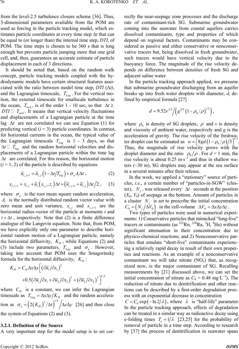

K. A. KOROTENKO ET AL.
76
from the level-2.5 turbulence closure scheme [36]. Thus,
3-dimensional parameters available from the POM are
used as forcing in the particle tracking model, which es-
timates particle coordinates at every time step Δt that can
be equal to (or longer than) the internal time step, DTI, of
POM. The time steps is chosen to be 360 s that is long
enough but prevents particle jumping more that one grid
cell, and, thus, guarantees an accurate estimate of particle
displacement in each of 3 directions.
It should be noted that, based on the random walk
concept, particle tracking models coupled with the hy-
drodynamic models have certain structural features asso-
ciated with the ratio between model time step, DTI (Δt),
and the Lagrangian timescale,
L
ag . For the vertical mo-
tion, the external timescale for smallscale turbulence in
the ocean, turb, is of the order 1 - 10 sec, so that
T
T t


turb . It means that vertical velocity fluctuations
and displacements of a Lagrangian particle at the time
lag are not correlated we can use Equation (1) for
predicting vertical (i = 3) particle coordinates. In contrast,
for horizontal currents in the ocean, the typical value of
the Lagrangian timescale
DTI T
t
L
ag
T is 1 - 3 days, so that
lag and the random horizontal velocities and dis-
placements of a Lagrangian particle within the time lag
are correlated. For this reason, the horizontal motion
(i = 1, 2) of the particle is described by equations
tT 
t

,1, 1 ijijlaga i
uu tTA 
t, (2)

,1,,,1 ,
,
ijijiij iijij2
x
xuxztuut

 , (3)
where a

is the root mean square random acceleration,
i
A
is the normally distributed random vector value with
zero mean and unit variance, ,ij
x
and ,1ij
x
 are the
horizontal radius-vector of the particle at moments t and
, respectively. Note that (2) is a finite difference
analogue of the Langevin equation. Note that, from POM,
we have explicitly only one parameter to describe hori-
zontal random motion of a Lagrangian particle, namely
the horizontal diffusivity,
tt
H
K
, while Equations (2) and
(3) include two parameters,
L
ag
T and a

. However,
taking into account that POM uses the Smagorinsky
formula for the horizontal diffusivity,
H
K
:


2
11
1/2
22
112 22 2
0.5
HH
KCxyux
ux uxux





where
H
C is a constant, we can infer the Lagrangian
timescale as
L
ag H
TxyK  and the random accelera-
tion as


1/2
3
2
aH
K
tx  y [26] and thus close
the system of Equations (2) and (3).
3.2.1. Definitio n of the Source
A very important step for the model setup is to set cor-
rectly the near-seepage zone processes and the discharge
rate of contaminant-rich SG. Submarine groundwater
coming into the seawater from coastal aquifers carries
dissolved contaminants, type and properties of which
depend on regional factors. Contaminants may be con-
sidered as passive and either conservative or nonconser-
vative tracers but, being dissolved in fresh groundwater,
such tracers would have vertical velocity due to the
buoyancy force. The magnitude of the rise velocity de-
pends on difference between densities of fresh SG and
adjacent saline water.
In the particle tracking approach applied, we presume
that submarine groundwater discharging from an aquifer
breaks up into fresh water droplets with diameter, d, de-
fined by empirical formula [27]



1/3
2/3 2/3
0
9.52 1dg   
,
where 0

is density of SG droplets,

and ν is density
and viscosity of ambient water, respectively and g is the
acceleration of gravity. The rise velocity of the freshwa-
ter droplet can be estimated as

1/ 2
0
81 3wgd   

.
Thus, the magnitude of rise velocity grows with the
droplet diameter and the ratio 0

. For d = 1 mm, the
rise velocity is about 0.25 m·s–1 and thus in shallow wa-
ters (~30 m), SG droplets may appear at the sea surface
in a several minutes after their release.
In the work, we applied a “stationary” source of parti-
cles, i.e., a certain number of “particles-in-SGW” (clus-
ter),
j
N, was released every seconds at the position
(X0, Y0) of seepage at the bottom. Amount of particles in
a cluster
t
j
N is set to prescribe the initial concentration


V
0
CN0j0
Two types of particles were used in numerical experi-
ments: 1) Conservative particles that mimicked “long-live”
tracers or contaminants (as 222Rn, 226Ra, 3H, 4He) without
significant attenuation in their concentration due to
physico-chemical reactions; and 2) Nonconservative par-
ticles that emulate “short-live” contaminants experienc-
ing a relatively rapid decay in result of their own proper-
ties and reactions. As an example of a nonconservative
contaminant we will take nitrate (NO3) that, as recog-
nized now, is the major contaminant of SG. Recalling
measurements by [21] discussed above, we can set the
initial concentration of nitrate as C0 = 0.48 mg·L–1), The
reduction of nitrate due to denitrification and other reac-
tions can be described by a first-order degradation proc-
ess with an exponential decrease in concentration
in the cell-volume . Vxyz


0expln 2CC

 , where

is “half-life” parameter.
In the particle tracking approach, effects of degradation
can be treated in a similar way as radioactive decay using
e-folding times 1
e
T


[23,25] for the probability of
removal of particle in a time step. According to research
by [37] the process of denitrification in seawater spans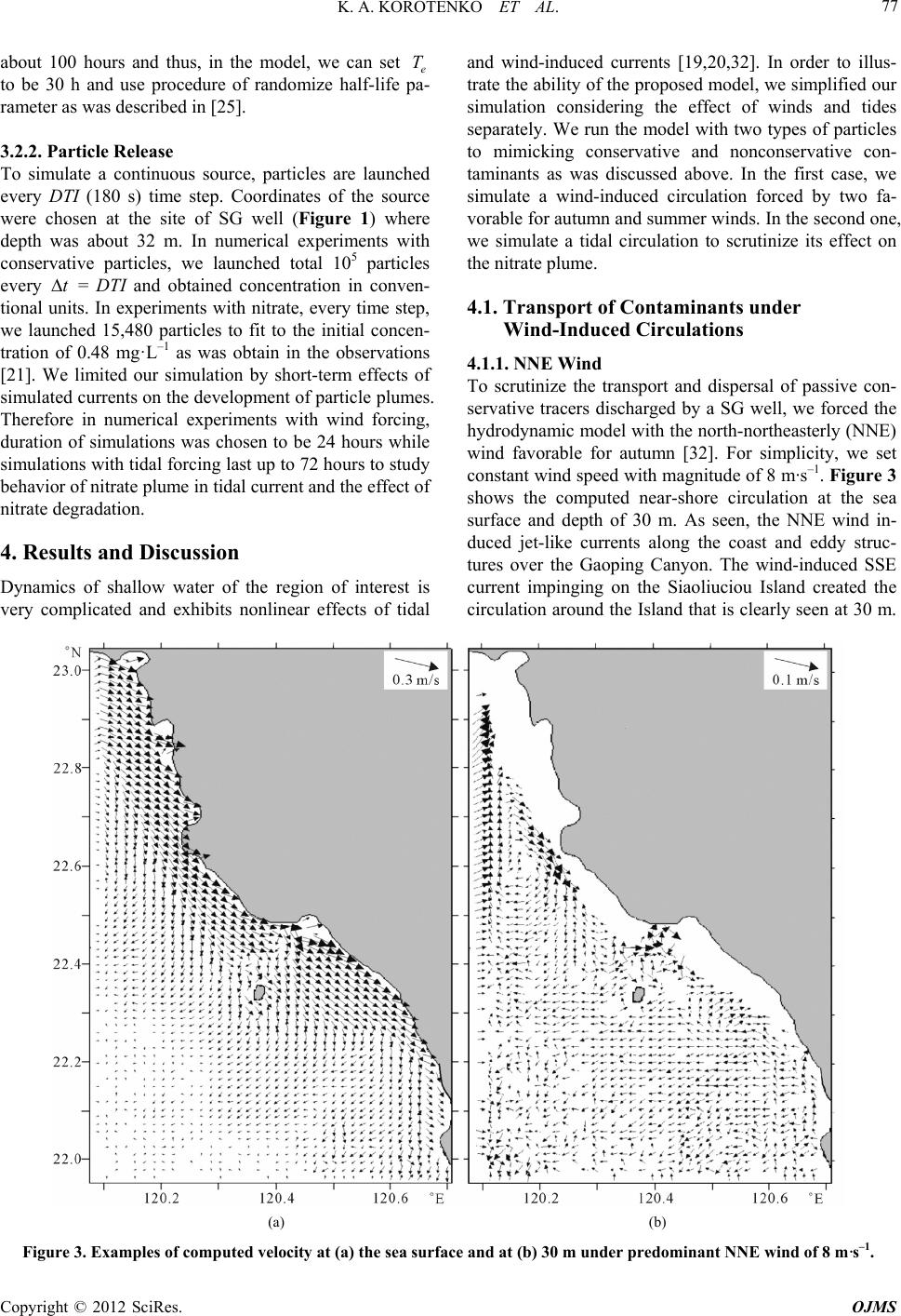

K. A. KOROTENKO ET AL.
77
about 100 hours and thus, in the model, we can set e
to be 30 h and use procedure of randomize half-life pa-
rameter as was described in [25].
T
3.2.2. Particle Re l e a se
To simulate a continuous source, particles are launched
every DTI (180 s) time step. Coordinates of the source
were chosen at the site of SG well (Figure 1) where
depth was about 32 m. In numerical experiments with
conservative particles, we launched total 105 particles
every t = DTI and obtained concentration in conven-
tional units. In experiments with nitrate, every time step,
we launched 15,480 particles to fit to the initial concen-
tration of 0.48 mg·L–1 as was obtain in the observations
[21]. We limited our simulation by short-term effects of
simulated currents on the development of particle plumes.
Therefore in numerical experiments with wind forcing,
duration of simulations was chosen to be 24 hours while
simulations with tidal forcing last up to 72 hours to study
behavior of nitrate plume in tidal current and the effect of
nitrate degradation.

4. Results and Discussion
Dynamics of shallow water of the region of interest is
very complicated and exhibits nonlinear effects of tidal
and wind-induced currents [19,20,32]. In order to illus-
trate the ability of the proposed model, we simplified our
simulation considering the effect of winds and tides
separately. We run the model with two types of particles
to mimicking conservative and nonconservative con-
taminants as was discussed above. In the first case, we
simulate a wind-induced circulation forced by two fa-
vorable for autumn and summer winds. In the second one,
we simulate a tidal circulation to scrutinize its effect on
the nitrate plume.
4.1. Transport of Contaminants under
Wind-Induced Circulations
4.1.1. N NE Wind
To scrutinize the transport and dispersal of passive con-
servative tracers discharged by a SG well, we forced the
hydrodynamic model with the north-northeasterly (NNE)
wind favorable for autumn [32]. For simplicity, we set
constant wind speed with magnitude of 8 m·s–1. Figure 3
shows the computed near-shore circulation at the sea
surface and depth of 30 m. As seen, the NNE wind in-
duced jet-like currents along the coast and eddy struc-
tures over the Gaoping Canyon. The wind-induced SSE
current impinging on the Siaoliuciou Island created the
circulation around the Island that is clearly seen at 30 m.
(a) (b)
Figure 3. Examples of computed velocity at (a) the sea surface and at (b) 30 m under predominant NNE wind of 8 m·s–1.

K. A. KOROTENKO ET AL.
78
At the surface, current velocity magnitude reached 0.3
m·s –1 while at 30 m the magnitude was about 0.1 m·s–1.
At 30 m, the circulation revealed distinct onshore flow at
the easternmost end of the Gaoping Canyon. Velocity
profiles (not shown here) indicated a veering of velocity
throughout the water column near the site of interest.
Figure 4 presents a planar plot of the integral2 con-
centration, C(x, y)H, of particles in 24 hours after their
release. Under NNE wind, the particles moved to south-
east along the coast, although some particles, as seen,
moved side- and backward due to the inhomogeneous
structure of the current velocity. Length and width of the
integral plume were about 15 and 7 km, respectively.
There were two maxima of concentration indicated the
slope of the particle plume that is clearly seen in Figure
5.
Presented in Figure 5, the 2-D cumulative X-Z and
Y-Z transections of the concentration give characteristic
details of vertical structure of the particle plume formed
in 24 h after their release. Here, “cumulative” means a
sum of all particles swept by the X-Z (Y-Z) area moving
along the Y (X) axis.
The asymmetric vertical structure of the plume was
associated with shear effects of wind-induced currents on
the vertical transport and dispersal of rising particles.
4.1.2. SS E Wind
The second numerical experiment was performed under
summer favorable wind, which, according to [32], blows
from south-southeast (SSE). Similarly to the previous
experiment, wind speed was chosen to be of 8 m/s.
As seen in Figure 6, the SSE wind induced strong
jet-like currents at the sea surface (cf. Figure 3) and
partly at 30 m. A weak distortion of the surface currents
occurred over the Gaoping Canyon while the strong cha-
otic circulation was at depth of 30 m indicated a signifi-
cant influence of the steep structure of the Canyon on the
current
Figure 7 shows the integral particle concentration dis-
tribution formed under the SSE wind of 8 m·s–1 in 24 h
after their release. As seen, the area covered by particles
was larger than that formed under the NNE wind; the
surface plume reached the Gaoping River estuary. Length
and width of the integral plume were about 17 and 8 km,
respectively. The maximum of particle concentration, as
seen, was near the source location.
Figure 8 presents the X-Z and Y-Z transections of
particle concentration. As in the experiment with SSE
wind, the concentration maximum was found to be at 3 -
4 m above the bottom indicating that the particle accu-
mulation increased when the rise of particles was re-
tarded. In contrast to the plume formed under NNE wind,
Figure 4. Integral concentrations of particles formed under
NNE wind of 8 m·s–1 after 24 h of discharge.
(a) (b)
Figure 5. The X-Z (a) and Y-Z (b) transections through a
particle plume relatively source coordinates (X0, Y0); the
experiment with NNE wind of 8 m·s–1.
in this case, the plume asymmetry indicated that margins
with lower gradients of particle concentrations are ex-
tended to the west (negative X) and to the north (positive
Y) from the source location.
4.2. Transport and Dispersal of Nitrate in Tidal
Current
The groundwater discharging into the sea often contains
nitrate with high concentrations. However, denitrification
2C(x, y)H = (N/ΔV), where N-number of particles, ΔV = Δx·Δy·Hand
H
(x, y) is depth.

K. A. KOROTENKO ET AL. 79
(a) (b)
Figure 6. Examples of computed velocity at (a) the sea surface and (b) 30 m under predominant SSE wind of 8 m·s–1.
Figure 7. Integral concentration of particles formed under
SSE wind of 8 m·s–1 after 24 h of discharge.
(a) (b)
Figure 8. The X-Z (a) and Y-Z (b) transections through a
particle plume relatively source coordinates (X0, Y0); the
experiment with SSE wind of 8 m·s –1.
and dilution of nitrate apparently reduces its concentra-
tion. As measurements indicated [37], the attenuation of
nitrate concentration in the seawater proceeds quite rap-
idly. Of interest here is to estimate scales of the nitrate
contamination of adjacent seawater nearby the SG well

K. A. KOROTENKO ET AL.
80
as well study an influence of tidal circulation on the dis-
tribution of nitrate in the impacted zone. For this, we
forced the hydrodynamic model with dominant constitu-
ent M2 and tune the model to adjust computed current
velocity to that obtained in the field observations with
ADCP [38].
Figure 9 presents the time series of horizontal velocity
components, U and V, and horizontal, KH, and vertical
diffusivities, KV, at 15 m above the bottom. As seen, KH
and KV exhibit significant variation during the tidal cycle
with KH ranges from about 4 to 20 m2·s–1 and KV ranges
from about 10–4 to 10–2 m
2·s–1 that is very close to KV
derived from direct measurements of turbulence obtained
with a high-frequency ADCP in tidal bottom layer [38].
Minima of the viscosities lag the minima of the current
velocity; the time lag is about 1.5 h.
Figure 10 illustrates successive phases of the nitrate
plume evolution in the tidal current. For the parameters
of the model initialization, nitrate reached the sea surface
in about 3 min after its release. Tidal oscillations cause to
periodic variations of the plume position relatively the
vertical axis. An asymmetry of current velocity and tur-
bulent diffusivities echoes in the nitrate plume structure
and variability in the water column.
As seen in Figure 10, the curvature of the plume is
more pronounced when the tidal current directed to the
southeast. The equalization of nitrate concentration level
comes after 24 h. Before, we see the vertical extension of
the high concentration core (~10–1 mg·L–1) of the plume.
Figure 11 shows the integral nitrate concentration
formed under tidal circulation in 24 h after nitrate release.
As seen, the area occupied by particles is noticeably less
than those formed in the experiments with NNE and SSE
winds, and particles are mostly dispersed around the
source point, through the northwestward drift is clearly
seen.
5. Summary
Although submarine springs and seeps around Taiwan
have been known for many years, these features have
traditionally been perceived as hydrologic “curiosities”
rather than objects for serious scientific investigation.
Despite low volume (relatively the riverine input) of
SGD inputs into coastal waters of the southwestern Tai-
wan, SGDs are recognized as potentially significant
sources of various pollutants.
An assessment of SGD-originated contamination im-
pact on ecosystems requires a complex approach to this
problem including experimental study and numerical
modeling. Until now, numerical modeling focused on the
solution of problems associated with contaminant distri-
bution inside aquifers and only a few works focused on
the processes near-seepage zones. In the paper, we pre-
sented the 3-D coupled circulation/particle transport model
for predicting coastal circulation and its effect on the
transport and distribution of particles mimicking conser-
vative and nonconservative (nitrate) contaminants dis-
charging in seawater in result of seepage of submarine
groundwater.
To our knowledge, this couple model is the first one
that was developed for such specific problems. Numeri-
cal experiments were performed with favorable for au-
tumn and summer winds and under simplified tidal cir-
culation forced only by M2 constituent. However, the
model gave reasonable results for scales and distributions
of discharged particles/contaminants in shallow zone
under the applied forcing. It is worthwhile to note that
Figure 9. Tidal cycle of computed velocity components, U and V (both in m·s–1), vertical = and horizontal diffu-
sivities = K
H/40 (both in m2·s–1) at 15 m above the bottom.
*
V
K50
*
V
K
*
H
K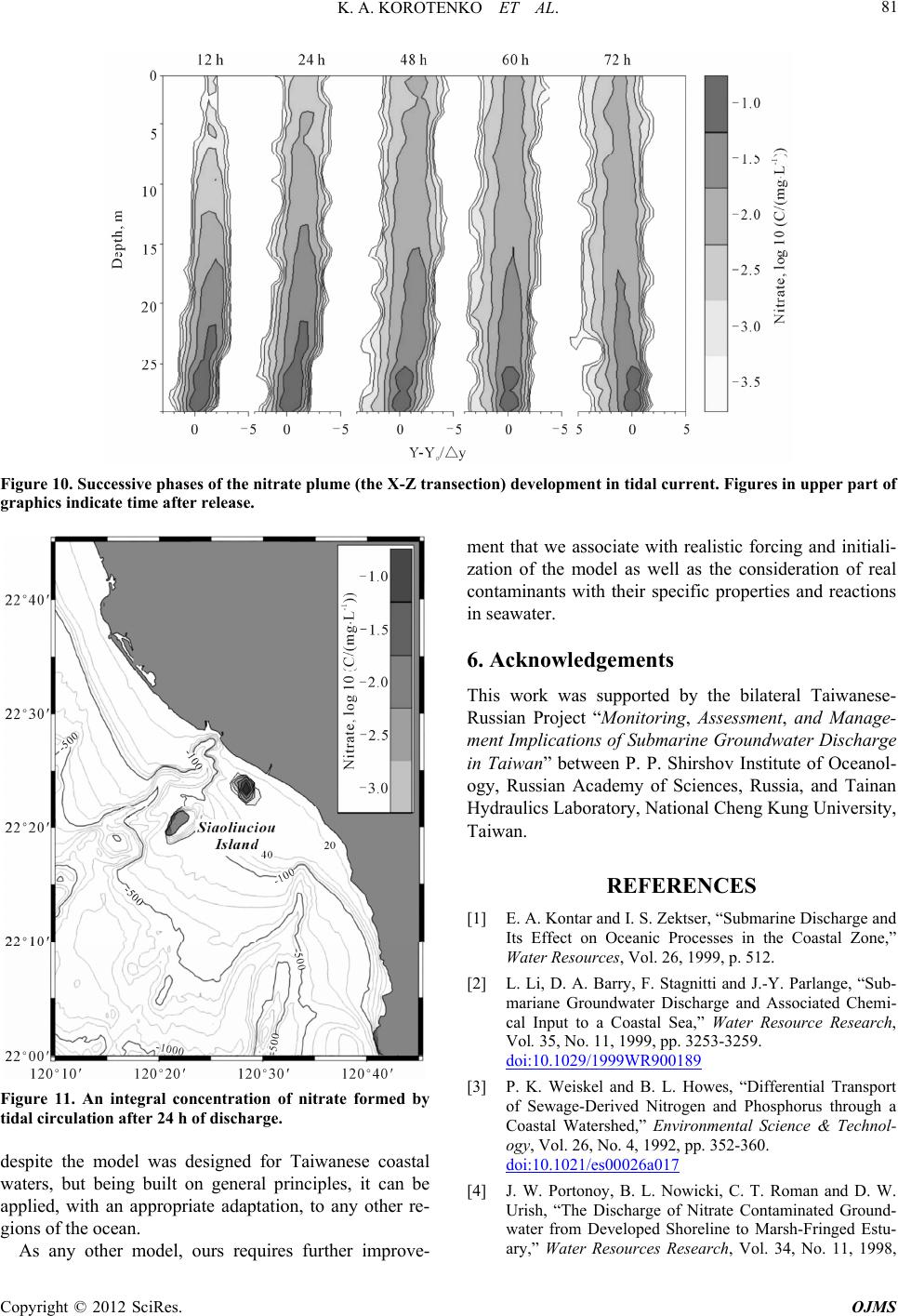

K. A. KOROTENKO ET AL. 81
Figure 10. Successive phases of the nitrate plume (the X-Z transection) development in tidal current. Figures in upper part of
graphics indicate time after release.
Figure 11. An integral concentration of nitrate formed by
tidal circulation after 24 h of discharge.
despite the model was designed for Taiwanese coastal
waters, but being built on general principles, it can be
applied, with an appropriate adaptation, to any other re-
gions of the ocean.
As any other model, ours requires further improve-
ment that we associate with realistic forcing and initiali-
zation of the model as well as the consideration of real
contaminants with their specific properties and reactions
in seawater.
6. Acknowledgements
This work was supported by the bilateral Taiwanese-
Russian Project “Monitoring, Assessment, and Manage-
ment Implications of Submarine Groundwater Discharge
in Taiwan” between P. P. Shirshov Institute of Oceanol-
ogy, Russian Academy of Sciences, Russia, and Tainan
Hydraulics Laboratory, National Cheng Kung University,
Taiwan.
REFERENCES
[1] E. A. Kontar and I. S. Zektser, “Submarine Discharge and
Its Effect on Oceanic Processes in the Coastal Zone,”
Water Resources, Vol. 26, 1999, p. 512.
[2] L. Li, D. A. Barry, F. Stagnitti and J.-Y. Parlange, “Sub-
mariane Groundwater Discharge and Associated Chemi-
cal Input to a Coastal Sea,” Water Resource Research,
Vol. 35, No. 11, 1999, pp. 3253-3259.
doi:10.1029/1999WR900189
[3] P. K. Weiskel and B. L. Howes, “Differential Transport
of Sewage-Derived Nitrogen and Phosphorus through a
Coastal Watershed,” Environmental Science & Technol-
ogy, Vol. 26, No. 4, 1992, pp. 352-360.
doi:10.1021/es00026a017
[4] J. W. Portonoy, B. L. Nowicki, C. T. Roman and D. W.
Urish, “The Discharge of Nitrate Contaminated Ground-
water from Developed Shoreline to Marsh-Fringed Estu-
ary,” Water Resources Research, Vol. 34, No. 11, 1998,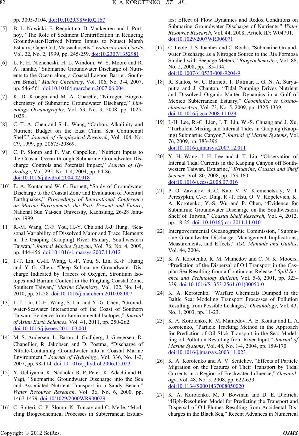

K. A. KOROTENKO ET AL.
82
pp. 3095-3104. doi:10.1029/98WR02167
[5] B. L. Nowicki, E. Requintina, D. Vankeuren and J. Port-
noy, “The Role of Sediment Denitrification in Reducing
Groundwater-Derived Nitrate Inputs to Nauset Marsh
Estuary, Cape Cod, Massachusetts,” Estuaries and Coasts,
Vol. 22, No. 2, 1999, pp. 245-259. doi:10.2307/1352981
[6] L. F. H. Niencheski, H. L. Windom, W. S. Moore and R.
A. Jahnke, “Submarine Groundwater Discharge of Nutri-
ents to the Ocean along a Coastal Lagoon Barrier, South-
ern Brazil,” Marine Chemistry, Vol. 106, No. 3-4, 2007,
pp. 546-561. doi.10.1016/j.marchem.2007.06.004
[7] K. D. Kroeger and M. A. Charette, “Nitrogen Biogeo-
chemistry of Submarine Groundwater Discharge,” Lim-
nology Oceanography, Vol. 53, No. 3, 2008, pp. 1025-
1039.
[8] C.-T. A. Chen and S.-L. Wang, “Carbon, Alkalinity and
Nutrient Budget on the East China Sea Continental
Shelf,” Journal of Geophysical Research, Vol. 104, No.
C9, 1999, pp. 20675-20869.
[9] C. P. Slomp and P. Van Cappellen, “Nutrient Inputs to
the Coastal Ocean through Submarine Groundwater Dis-
charge: Controls and Potential Impact,” Journal of Hy-
drology, Vol. 295, No. 1-4, 2004, pp. 64-86.
doi:10.1016/j.jhydrol.2004.02.018
[10] E. A. Kontar and W. C. Burnett, “Study of Groundwater
Discharge to the Coastal Zone and Evaluation of Potential
Earthquakes,” Proceedings of International Conference
on Marine Environment, the Past, Present and Future,
National Sun Yat-sen University, Kaohsiung, 26-28 Janu-
ary 1999.
[11] R.-M. Wang, C.-F. You, H.-Y. Chu and J.-J. Hung, “Sea-
sonal Variability of Dissolved Major and Trace Elements
in the Gaoping (Kaoping) River Estuary, Southwestern
Taiwan,” Journal Marine Systyem, Vol. 76, No. 4, 2009,
pp. 444-456. doi:10.1016/j.jmarsys.2007.11.012
[12] I.-T. Lin, C.-H. Wang, C.-F. You, S. Lin, K.-F. Huang
and Y.-G. Chen, “Deep Submarine Groundwater Dis-
charge Indicated by Tracers of Oxygen, Strontium Iso-
topes and Barium Content in the Pingtung Coastal Zone,
Southern Taiwan,” Marine Chemistry, Vol. 122, No. 1-4,
2010, pp. 51-58. doi:10.1016/j.marchem.2010.08.007
[13] I.-T. Lin, C.-H. Wang, S. Lin and Y.-G. Chen, “Ground-
water-Seawater Interactions off the Coast of Southern
Taiwan: Evidence from Environmental Isotopes,” Journal
of Asian Earth Sciences, Vol. 41, 2011, pp. 250-262.
doi:10.1016/j.jseaes.2011.03.001
[14] M. S. Andersen, L. Baron, J. Gudbjerg, J. Gregersen, D.
Chapellier, R. Jakobsen and D. Postma, “Discharge of
Nitrate-Containing Groundwater into a Coastal Marine
Environment,” Journal of Hydrology, Vol. 336, No. 1-2,
2007, pp. 98-114. doi:10.1016/j.jhydrol.2006.12.023
[15] Y. Uchiyama, K. Nadaoka, R. P. Peter, K. Adachi and H.
Yagi, “Submarine Groundwater Discharge into the Sea
and Associated Nutrient Transport in a Sandy Beach,”
Water Resource Research, Vol. 36, No. 6, 2000, pp.
1467-1479. doi:10/1029/2000WR900029
[16] C. Spiteri, C. P. Slomp, K. Tuncay and C. Meile, “Mod-
eling Biogeochemical Processes in Subterranean Estuar-
ies: Effect of Flow Dynamics and Redox Conditions on
Submarine Groundwater Discharge of Nutrients,” Water
Resource Research, Vol. 44, 2008, Article ID: W04701.
doi:10.1029/2007WR006071
[17] C. Leote, J. S. Ibanhez and C. Rocha, “Submarine Ground-
water Discharge as a Nitrogen Source to the Ria Formosa
Studied with Seepage Meters,” Biogeochemistry, Vol. 88,
No. 2, 2008, pp. 185-194.
doi:10.1007/s10533-008-9204-9
[18] R. Santos, W. C. Burnett, T. Dittmar, I. G. N. A. Surya-
putra and J. Chanton, “Tidal Pumping Drives Nutrient
and Dissolved Organic Matter Dynamics in a Gulf of
Mexico Subterranean Estuary,” Geochimica et Cosmo-
chimica Acta, Vol. 73, No. 5, 2009, pp. 1325-1339.
doi:10.1016/j.gca.2008.11.029
[19] I.-H. Lee, R.-C. Lien, J. T. Liu, W.-S. Chuang and J. Xu,
“Turbulent Mixing and Internal Tides in Gaoping (Kaop-
ing) Submarine Canyon,” Journal of Marine Systems, Vol.
76, 2009, pp. 383-396.
doi:10.1016/j.jmarsys.2007.12.011
[20] Y. H. Wang, I. H. Lee and J. T. Liu, “Observation of
Internal Tidal Currents in the Kaoping Canyon off South-
western Taiwan. Estuarine,” Estuarine, Coastal and Shelf
Science, Vol. 80, 2008, pp. 153-160.
doi:10.1016/j.ecss.2008.07.016
[21] P. O. Zavialov, R.-C. Kao, V. V. Kremenetskiy, V. I.
Peresypkin, C.-F. Ding, R.-T. Hsu, O. V. Kopelevich, K.
A. Korotenko, Y.-S. Wu and P. Chen, “Evidence for
Submarine Groundwater Discharge on the Southwestern
Shelf of Taiwan,” Coastal Shelf Research, Vol. 4, 2012,
pp. 18-25. doi: 10.1016/j.csr.2011.11.010
[22] Intergovernmental Oceanographic Commission, “Subma-
rine Groundwater Discharge: Management Implications,
Measurements, and Effects,” IOC Manuals and Guides,
Vol. 44, 2004.
[23] K. A. Korotenko, R. M. Mamedov and C. N. K. Mooers,
“Prediction of the Dispersal of Oil Transport in the Cas-
pian Sea Resulting from a Continuous Release,” Spill Sci-
ence and Technology Bulletin, Vol. 5-6, 2001, pp. 323-
339. doi:10.1016/S1353-2561 (01)00050-0
[24] K. A. Korotenko, “Warfare Chemicals Dumped in the
Baltic Sea: Modeling Transport Processes of Pollution
Resulting from Possible Leakages,” Oceanology, Vol. 43,
No. 1, 2003, pp. 11-23.
[25] K. A. Korotenko, R. M. Mamedov, A. E. Kontar and L. A.
Korotenko, “Particle Tracking Method in the Approach
for Prediction of Oil Slick Transport in the Sea: Model-
ling oil Pollution Resulting from River Input,” Journal of
Marine Systems, Vol. 48, No. 1-4, 2004, pp. 159-170.
doi:10.1016/j.jmarsys.2003.11.023
[26] K. A. Korotenko and A. V. Sentchev, “Effects of Particle
Migration on the Features of Their Transport by Tidal
Currents in a Region of Freshwater Influence,” Oceanol-
ogy, Vol. 48, No. 5, 2008, pp. 622-633.
doi:10.1134/S0001437008050020
[27] K. A. Korotenko, M. J. Bowman and D. E. Dietrich,
“High-Resolution Model for Predicting the Transport and
Dispersal of Oil Plumes Resulting from Accidental Dis-
charges in the Black Sea,” Recent Advances in Numerical

K. A. KOROTENKO ET AL.
83
Ocean Modeling and Prediction, Terrestrial Atmospheric
and Oceanic Sciences, Vol. 21, 2010, pp. 123-136.
doi:10.3319/TAO.2009.04.24.01(IWNOP)
[28] V. Sentchev and K. A. Korotenko, “Stratification and
Tidal Current Effects on Larval Transport in the Eastern
English Channel: Observations and 3D Modeling,” Envi-
ronmental Fluid Mechanics, Vol. 4, No. 3, 2004, pp.
305-331. doi:10.1023/B:EFMC.0000024246.39646.1d
[29] V. Sentchev and K. A. Korotenko, “Dispersion Processes
and Transport Pattern in the ROFI System of the Eastern
English Channel Derived from a Particle-Tracking Model,”
Continental Shelf Research, Vol. 25, No. 16, 2005, pp.
2294-2308. doi:10.1016/j.csr.2005.09.003
[30] V. Sentchev and K. A. Korotenko, “Modeling Distribu-
tion of Flounder Larvae in the Eastern English Channel:
Sensitivity to Physical Forcing and Biological Behavior,”
Marine Ecology Progress Series, Vol. 347, 2007, pp.
233-245. doi:10.3354/meps06981
[31] F. Blumberg and G. L. Mellor, “A Description of a
Three-Dimensional Hydrodynamic Model of New York
Harbor Region,” Journal Hydraulic Engineering, Vol.
125, 1987, pp. 799-816.
[32] B. W. J. Kern, Y.-L. Chen and M.-Y. Chang, “The Diur-
nal Cycle of Winds, Rain, and Clouds over Taiwan during
the Mey-Yu, Summer, and Autumn Rainfall Regimes,"
Monthly Weather Review, Vol. 138, No. 2, 2010, pp.
497-516. doi:10.1175/2009MWR3031.1
[33] S. Levitus, “World Ocean Atlas//NOAA Atlas,” US De-
partment of Commerce. NOAA/NODC, 2009.
[34] J. Hunter, C. Craig and H. Phillips, “On the Use of Ran-
dom-Walk Models with Spatially-Variable Diffusivity,”
Journal of Computational Physics, Vol. 106, No. 2, 1993,
pp. 366-376. doi:10.1016/S0021- 9991(83)71114-9
[35] A. Visser, “Using Random Walk Models to Simulate the
Vertical Distribution of Particles in a Turbulent Water
Column,” Marine Ecology Progress Series, Vol. 158,
1997, pp. 275-281. doi:10.3354/meps15827
[36] G. L Mellor and T. Yamada, “Development of a Turbu-
lence Closure Model for Geophysical Fluid Problems,”
Review of Geophysics Space Physics, Vol. 20, No. 4,
1982, pp. 851-875. doi:10.1029/ RG020i004p00851
[37] J. J. Coering and J. D. Cline, “A Note on Denitrification
in Seawater,” Limnology and Oceanography, Vol. 15,
1970, pp. 306-309.
[38] K. A. Korotenko and A. V. Sentchev, “Turbulence Inves-
tigation in a Tidal Coastal Region,” Oceanology, Vol. 51,
No. 3, 2011, pp. 394-406.
doi:10.1134/S000143701103012X.
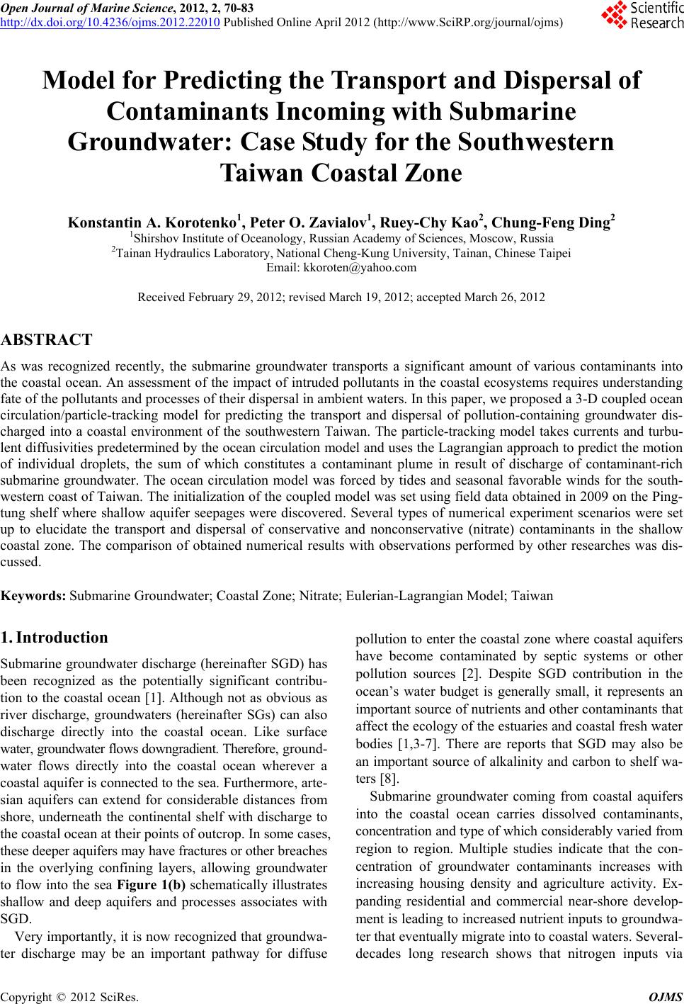