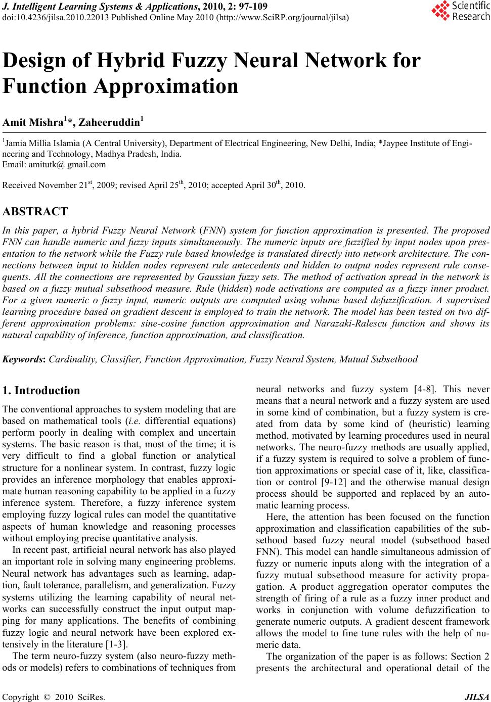J. Intelligent Learning Systems & Applications, 2010, 2: 97-109
doi:10.4236/jilsa.2010.22013 Published Online May 2010 (http://www.SciRP.org/journal/jilsa)
97
Design of Hybrid Fuzzy Neural Network for
Function Approximation
Amit Mishra1*, Zaheeruddin1
1Jamia Millia Islamia (A Central University), Department of Electrical Engineering, New Delhi, India; *Jaypee Institute of Engi-
neering and Technology, Madhya Pradesh, India.
Received November 21st, 2009; revised April 25th, 2010; accepted April 30th, 2010.
ABSTRACT
In this paper, a hybrid Fuzzy Neural Network (FNN) system for function approximation is presented. The proposed
FNN can handle numeric and fuzzy inputs simultaneously. The numeric inputs are fuzzified by input nodes upon pres-
entation to the network while the Fuzzy rule based knowledge is translated directly into network architecture. The con-
nections between input to hidden nodes represent rule antecedents and hidden to output nodes represent rule conse-
quents. All the connections are represented by Gaussian fuzzy sets. The method of activation spread in the network is
based on a fuzzy mutual subsethood measure. Rule (hidden) node activations are computed as a fuzzy inner product.
For a given numeric o fuzzy input, numeric outputs are computed using volume based defuzzification. A supervised
learning procedure based on gradient descent is employed to train the network. The model has been tested on two dif-
ferent approximation problems: sine-cosine function approximation and Narazaki-Ralescu function and shows its
natural capability of inference, function approximation, and classification.
Keywords: Cardinality, Classifier, Function Approximation, Fuzzy Neural System, Mutual Subsethood
1. Introduction
The conventional approaches to system modeling that are
based on mathematical tools (i.e. differential equations)
perform poorly in dealing with complex and uncertain
systems. The basic reason is that, most of the time; it is
very difficult to find a global function or analytical
structure for a nonlinear system. In contrast, fuzzy logic
provides an inference morphology that enables approxi-
mate human reasoning capability to be applied in a fuzzy
inference system. Therefore, a fuzzy inference system
employing fuzzy logical rules can model the quantitative
aspects of human knowledge and reasoning processes
without employing precise quantitative analysis.
In recent past, artificial neural network has also played
an important role in solving many engineering problems.
Neural network has advantages such as learning, adap-
tion, fault tolerance, parallelism, and generalization. Fuzzy
systems utilizing the learning capability of neural net-
works can successfully construct the input output map-
ping for many applications. The benefits of combining
fuzzy logic and neural network have been explored ex-
tensively in the literature [1-3].
The term neuro-fuzzy system (also neuro-fuzzy meth-
ods or models) refers to combinations of techniques from
neural networks and fuzzy system [4-8]. This never
means that a neural network and a fuzzy system are used
in some kind of combination, but a fuzzy system is cre-
ated from data by some kind of (heuristic) learning
method, motivated by learning procedures used in neural
networks. The neuro-fuzzy methods are usually applied,
if a fuzzy system is required to solve a problem of func-
tion approximations or special case of it, like, classifica-
tion or control [9-12] and the otherwise manual design
process should be supported and replaced by an auto-
matic learning process.
Here, the attention has been focused on the function
approximation and classification capabilities of the sub-
sethood based fuzzy neural model (subsethood based
FNN). This model can handle simultaneous admission of
fuzzy or numeric inputs along with the integration of a
fuzzy mutual subsethood measure for activity propa-
gation. A product aggregation operator computes the
strength of firing of a rule as a fuzzy inner product and
works in conjunction with volume defuzzification to
generate numeric outputs. A gradient descent framework
allows the model to fine tune rules with the help of nu-
meric data.
The organization of the paper is as follows: Section 2
presents the architectural and operational detail of the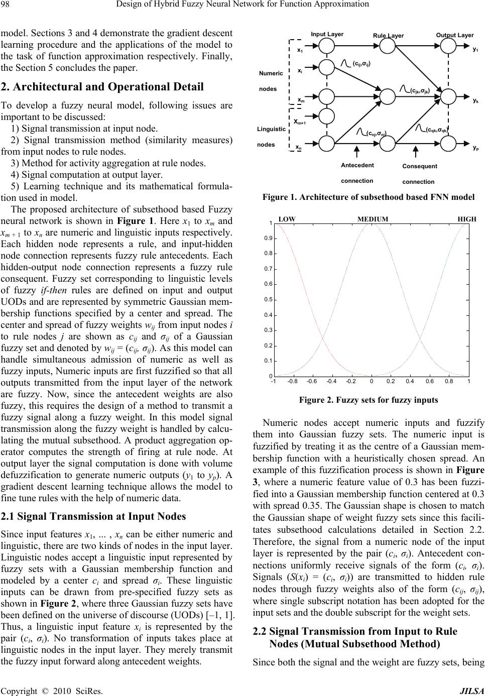

Design of Hybrid Fuzzy Neural Network for Function Approximation 98
model. Sections 3 and 4 demonstrate the gradient descent
learning procedure and the applications of the model to
the task of function approximation respectively. Finally,
the Section 5 concludes the paper.
2. Architectural and Operational Detail
To develop a fuzzy neural model, following issues are
important to be discussed:
1) Signal transmission at input node.
2) Signal transmission method (similarity measures)
from input nodes to rule nodes.
3) Method for activity aggregation at rule nodes.
4) Signal computation at output layer.
5) Learning technique and its mathematical formula-
tion used in model.
The proposed architecture of subsethood based Fuzzy
neural network is shown in Figure 1. Here x1 to xm and
xm + 1 to xn are numeric and linguistic inputs respectively.
Each hidden node represents a rule, and input-hidden
node connection represents fuzzy rule antecedents. Each
hidden-output node connection represents a fuzzy rule
consequent. Fuzzy set corresponding to linguistic levels
of fuzzy if-then rules are defined on input and output
UODs and are represented by symmetric Gaussian mem-
bership functions specified by a center and spread. The
center and spread of fuzzy weights wij from input nodes i
to rule nodes j are shown as cij and σij of a Gaussian
fuzzy set and denoted by wij = (cij, σij). As this model can
handle simultaneous admission of numeric as well as
fuzzy inputs, Numeric inputs are first fuzzified so that all
outputs transmitted from the input layer of the network
are fuzzy. Now, since the antecedent weights are also
fuzzy, this requires the design of a method to transmit a
fuzzy signal along a fuzzy weight. In this model signal
transmission along the fuzzy weight is handled by calcu-
lating the mutual subsethood. A product aggregation op-
erator computes the strength of firing at rule node. At
output layer the signal computation is done with volume
defuzzification to generate numeric outputs (y1 to yp). A
gradient descent learning technique allows the model to
fine tune rules with the help of numeric data.
2.1 Signal Transmission at Input Nodes
Since input features x1, ... , xn can be either numeric and
linguistic, there are two kinds of nodes in the input layer.
Linguistic nodes accept a linguistic input represented by
fuzzy sets with a Gaussian membership function and
modeled by a center ci and spread σi. These linguistic
inputs can be drawn from pre-specified fuzzy sets as
shown in Figure 2, where three Gaussian fuzzy sets have
been defined on the universe of discourse (UODs) [–1, 1].
Thus, a linguistic input feature xi is represented by the
pair (ci, σi). No transformation of inputs takes place at
linguistic nodes in the input layer. They merely transmit
the fuzzy input forward along antecedent weights.
x
1
x
i
x
m
X
m+1
x
n
Input Layer
Rule Layer Output Layer
Numeric
nodes
Linguistic
nodes
y
1
y
k
y
p
(c
ij
,σ
ij
)
(c
nj
,σ
nj
)
(c
jk
,σ
jk
)
(c
qk
,σ
qk
)
Antecedent
connection
Consequent
connection
Figure 1. Architecture of subsethood based FNN model
LOWMEDIUM HIGH
-1 -0.8 -0.6-0.4 -0.200.2 0.40.6 0.8 1
0
0.1
0.2
0.3
0.4
0.5
0.6
0.7
0.8
0.9
1
Figure 2. Fuzzy sets for fuzzy inputs
Numeric nodes accept numeric inputs and fuzzify
them into Gaussian fuzzy sets. The numeric input is
fuzzified by treating it as the centre of a Gaussian mem-
bership function with a heuristically chosen spread. An
example of this fuzzification process is shown in Figure
3, where a numeric feature value of 0.3 has been fuzzi-
fied into a Gaussian membership function centered at 0.3
with spread 0.35. The Gaussian shape is chosen to match
the Gaussian shape of weight fuzzy sets since this facili-
tates subsethood calculations detailed in Section 2.2.
Therefore, the signal from a numeric node of the input
layer is represented by the pair (ci, σi). Antecedent con-
nections uniformly receive signals of the form (ci, σi).
Signals (S(xi) = (ci, σi)) are transmitted to hidden rule
nodes through fuzzy weights also of the form (cij, σij),
where single subscript notation has been adopted for the
input sets and the double subscript for the weight sets.
2.2 Signal Transmission from Input to Rule
Nodes (Mutual Subsethood Method)
Since both the signal and the weight are fuzzy sets, being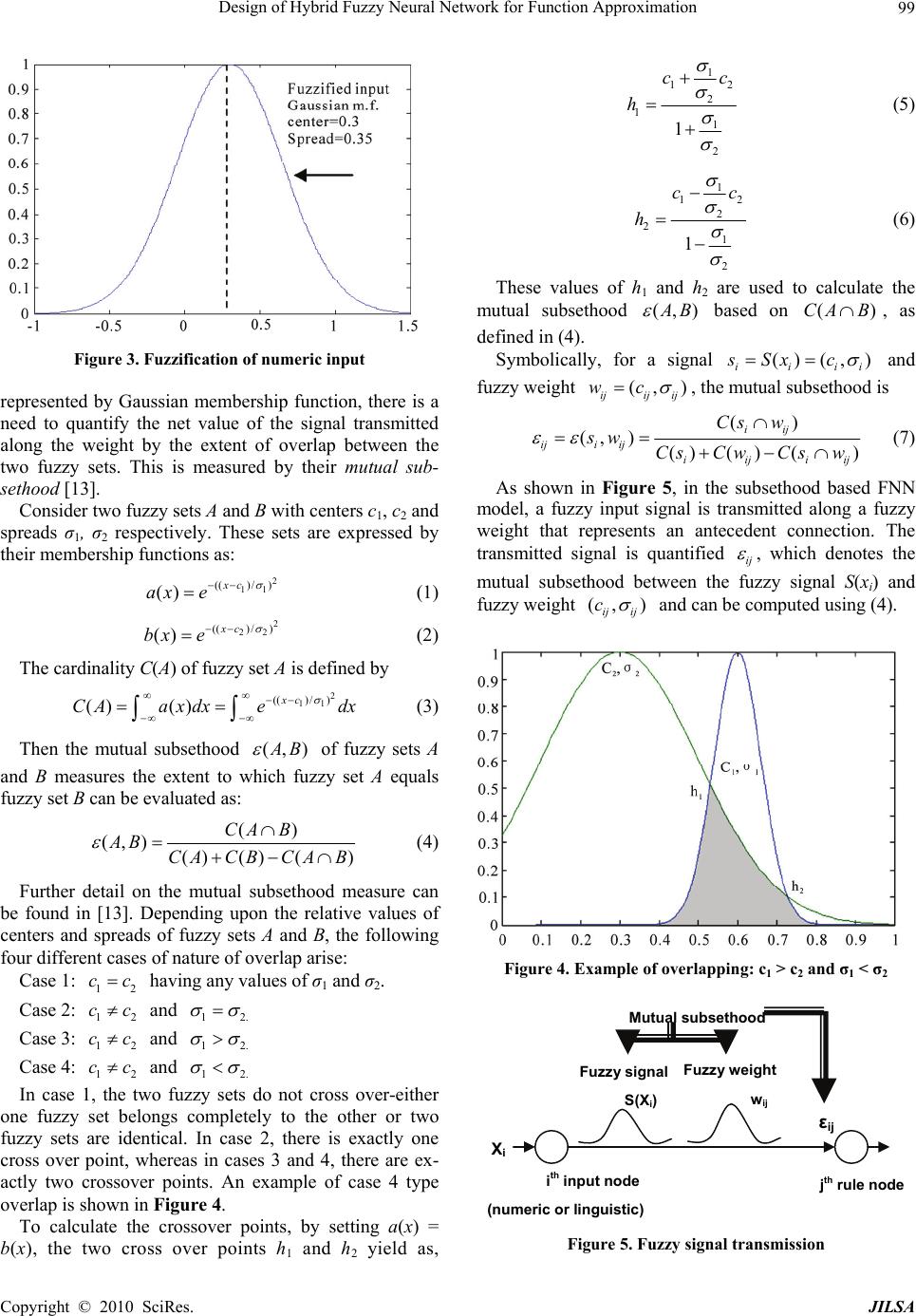

Design of Hybrid Fuzzy Neural Network for Function Approximation99
Figure 3. Fuzzification of numeric input
represented by Gaussian membership function, there is a
need to quantify the net value of the signal transmitted
along the weight by the extent of overlap between the
two fuzzy sets. This is measured by their mutual sub-
sethood [13].
Consider two fuzzy sets A and B with centers c1, c2 and
spreads σ1, σ2 respectively. These sets are expressed by
their membership functions as:
2
11
(()/ )
() xc ax e
 
 (1)
2
22
(()/ )
() xc bxe
 
 (2)
The cardinality C(A) of fuzzy set A is defined by
2
11
(()/ )
() ()xc CAaxdx edx



 

 (3)
Then the mutual subsethood (,)
A
B

of fuzzy sets A
and B measures the extent to which fuzzy set A equals
fuzzy set B can be evaluated as:
()
(,) () () ()
CA B
AB CACBCA B 

 (4)
Further detail on the mutual subsethood measure can
be found in [13]. Depending upon the relative values of
centers and spreads of fuzzy sets A and B, the following
four different cases of nature of overlap arise:
Case 1: having any values of σ1 and σ2.
1
cc2
2.
Case 2: and
1
cc12

 
Case 3: and
1
cc2.12

 
Case 4: and
1
cc2.12

 
In case 1, the two fuzzy sets do not cross over-either
one fuzzy set belongs completely to the other or two
fuzzy sets are identical. In case 2, there is exactly one
cross over point, whereas in cases 3 and 4, there are ex-
actly two crossover points. An example of case 4 type
overlap is shown in Figure 4.
To calculate the crossover points, by setting a(x) =
b(x), the two cross over points h1 and h2 yield as,
1
12
2
1
1
2
1
cc
h







(5)
1
12
2
2
1
2
1
cc
h







(6)
These values of h1 and h2 are used to calculate the
mutual subsethood (,)
A
B

based on (CA B)

, as
defined in (4).
Symbolically, for a signal () (, )
iii
sSx ci

 and
fuzzy weight (, )
ijij ij
wc


, the mutual subsethood is
()
(, )()( )()
iij
ijiij
iiji
Cs w
sw CsCwCsw 



ij
(7)
As shown in Figure 5, in the subsethood based FNN
model, a fuzzy input signal is transmitted along a fuzzy
weight that represents an antecedent connection. The
transmitted signal is quantified ij

, which denotes the
mutual subsethood between the fuzzy signal S(xi) and
fuzzy weight (, )
ij ij
c

and can be computed using (4).
Figure 4. Example of overlapping: c1 > c2 and σ1 < σ2
i
th
input node
(numeric or linguistic)
j
th
rule node
ε
ij
Fuzzy signal
S(X
i
)
Fuzzy weight
w
ij
Mutual subsethood
X
i
Figure 5. Fuzzy signal transmission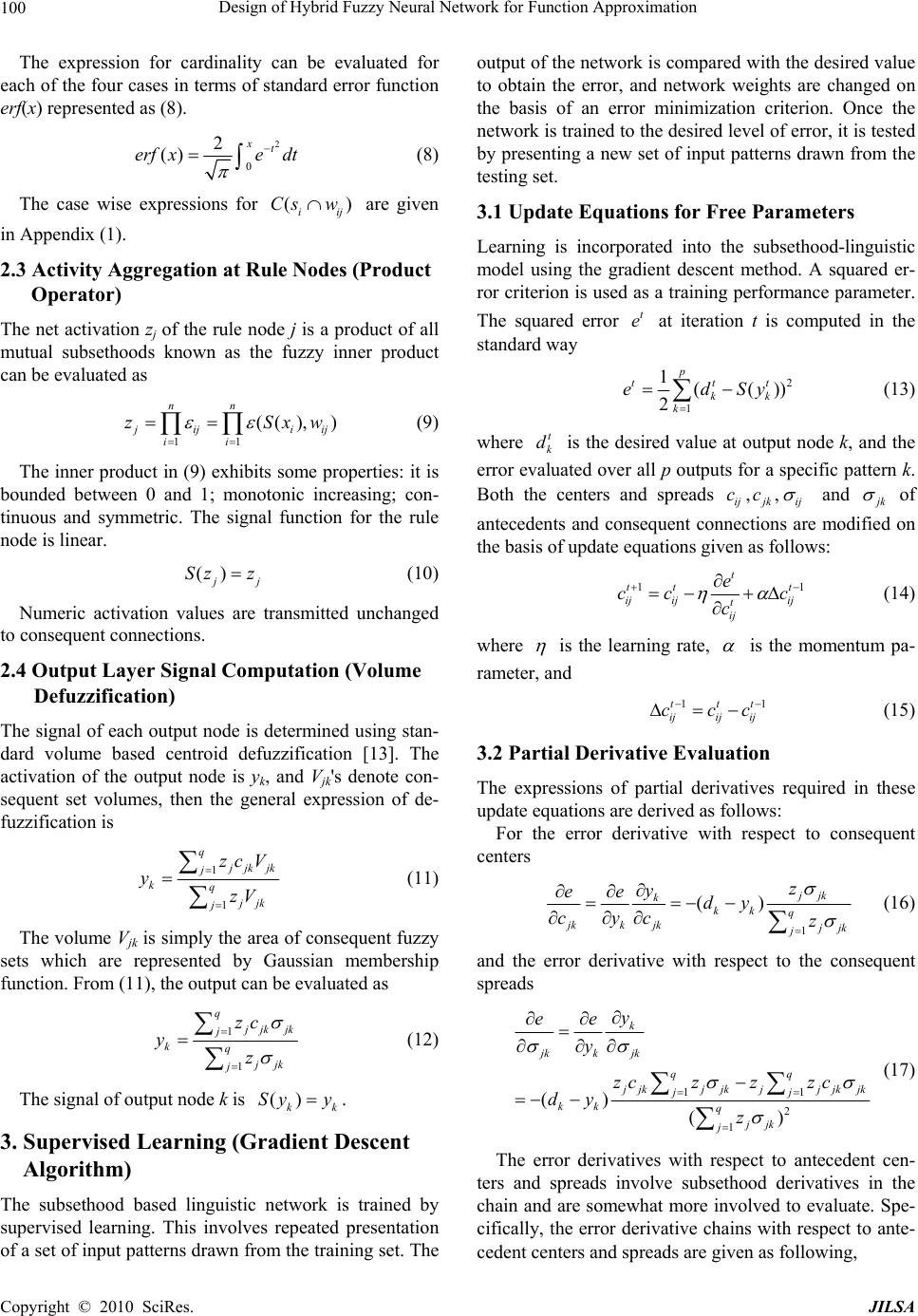

Design of Hybrid Fuzzy Neural Network for Function Approximation 100
The expression for cardinality can be evaluated for
each of the four cases in terms of standard error function
erf(x) represented as (8).
2
0
2
() xt erf xedt


 (8)
The case wise expressions for are given
in Appendix (1).
(
iij
Cs w)
2.3 Activity Aggregation at Rule Nodes (Product
Operator)
The net activation zj of the rule node j is a product of all
mutual subsethoods known as the fuzzy inner product
can be evaluated as
11
(( ),)
nn
j
iji ij
ii
zS 


xw (9)
The inner product in (9) exhibits some properties: it is
bounded between 0 and 1; monotonic increasing; con-
tinuous and symmetric. The signal function for the rule
node is linear.
()
j
j
Sz z

(10)
Numeric activation values are transmitted unchanged
to consequent connections.
2.4 Output Layer Signal Computation (Volume
Defuzzification)
The signal of each output node is determined using stan-
dard volume based centroid defuzzification [13]. The
activation of the output node is yk, and Vjk's denote con-
sequent set volumes, then the general expression of de-
fuzzification is
1
1
q
j
jk jk
j
kq
jjk
j
zc V
y
zV



 (11)
The volume Vjk is simply the area of consequent fuzzy
sets which are represented by Gaussian membership
function. From (11), the output can be evaluated as
1
1
q
j
jk jk
j
kq
jjk
j
zc
y
z





 (12)
The signal of output node k is . ()
kk
Sy y
3. Supervised Learning (Gradient Descent
Algorithm)
The subsethood based linguistic network is trained by
supervised learning. This involves repeated presentation
of a set of input patterns drawn from the training set. The
output of the network is compared with the desired value
to obtain the error, and network weights are changed on
the basis of an error minimization criterion. Once the
network is trained to the desired level of error, it is tested
by presenting a new set of input patterns drawn from the
testing set.
3.1 Update Equations for Free Parameters
Learning is incorporated into the subsethood-linguistic
model using the gradient descent method. A squared er-
ror criterion is used as a training performance parameter.
The squared error at iteration t is computed in the
standard way
t
e
2
1
1(()
2
p
tt
kk
k
edSy


)
t
(13)
where is the desired value at output node k, and the
error evaluated over all p outputs for a specific pattern k.
Both the centers and spreads
t
k
d
,,
ij jkij
cc

and
j
k

of
antecedents and consequent connections are modified on
the basis of update equations given as follows:
11
t
tt t
ij ijij
t
ij
e
cc c
c




 
 (14)
where

is the learning rate,

is the momentum pa-
rameter, and
1ttt
ijij ij
ccc
1


 (15)
3.2 Partial Derivative Evaluation
The expressions of partial derivatives required in these
update equations are derived as follows:
For the error derivative with respect to consequent
centers
1
()
jjk
k
kk q
jkk jk
j
jk
j
z
y ee dy
cyc z



 

  (16)
and the error derivative with respect to the consequent
spreads
11
2
1
()
()
k
jkk jk
qq
j
jkjjkjj jkjk
jj
kk q
jjk
j
y
ee
y
zczz zc
dy
z











 

(17)
The error derivatives with respect to antecedent cen-
ters and spreads involve subsethood derivatives in the
chain and are somewhat more involved to evaluate. Spe-
cifically, the error derivative chains with respect to ante-
cedent centers and spreads are given as following,

Design of Hybrid Fuzzy Neural Network for Function Approximation 101
1
1
()
pjij
k
k
ijkjij ij
p
j
ij
k
kk
k
j
ij ij
z
y ee
cyzc
z
y
dyzc







 




 




(18)


11
2
1
11
2
1
1
()
qq
j
kjkjjkjk jjkjk
jj
k
q
jjjk
j
qq
jkjjkj jkjk
jj
jk q
jjk
j
jk jkk
q
jjk
j
cz zc
y
zz
cz zc
z
cy
z

 



























(21)
1
1
()
pjij
k
k
ijkj ijij
p
j
ij
k
kk
k
j
ij ij
z
y ee
yz
z
y
dyz








 




 




(19)
and
and the error derivative chains with respect to input fea-
ture spread is evaluated as
1,
n
j
ij
iij
ij
z




 (22)
11
11
()
qp
j
ij
k
jk
j
kjij i
qp
j
ij
k
kk
jk
j
ij i
z
y ee
yz
z
y
dyz









 








(20) The expressions for antecedent connection, mutual
subsethood partial derivatives ij
ij
c


 and ij
ij



 are ob-
tained by differentiating (7) with respect to cij, σij and σi
as in (23), (24) and (25).
where


2
() ()
()() ()
()()
iij iij
iiji iji ij
ij ij
ij
ij iiji ij
Cs wCs w
Cs wCs w
cc
cCs w
 

 

  
 
 





 







(23)
2
() ()
(()( ))( )
(() ())
iij iij
ij iiijiij
ij ij
ij
ij ij iiij
Cs wCs w
Cs wCs w
Cs w
 


 



 
   

















(24)
2
() ()
(()( ))( )
(() ())
iij iij
ijii iji ij
i i ij
iij iiij
Cs wCs w
Cs wCs w
Cs w
 
 
 

 

 
 


 










ij
(25)
In these equations, the calculation of ()/
iij ij
Cs wc ,
()/
iij
Cs w

 and i ()/
iij
Cs w

  are require
which depends onature of overlap o
termining or learning depends on how
fin
d
the nf the input fea-
ture fuzzy set and weight fuzzy set. The case wise ex-
pressions are demonstrated in Appendix (2).
4. Function Approximation
Function approximation involves de
the input-output relations using numeric input-output
data. Conventional methods like linear regression are
useful in cases where the relation being learnt, is linear or
quasi-linear. For nonlinear function approximation mul-
tilayer neural networks are well suited to solve the prob-
lem but with the drawback of their black box nature and
heuristic decisions regarding network structure and tun-
able parameters. Interpretability of learnt knowledge in
conventional neural networks is a severe problem. On the
other hand, function approximation by fuzzy systems
employs the concept of dividing the input space into sub
regions, and for each sub region a fuzzy rule is defined
thus making the system interpretable.
The performance of the fuzzy system
ally the sub regions are generated. The practical imita-
tion arises with fuzzy systems when the input variables
are increased and the number of fuzzy rules explodes
leading to the problem known as the curse of dimension-
ality. It is now well known that both fuzzy system and

Design of Hybrid Fuzzy Neural Network for Function Approximation 102
neural network are universal function approximators and
can approximate functions to any arbitrary degree of ac-
curacy [13,14]. Fuzzy neural system also has capability
of approximating any continuous function or modeling a
system [15-17].
There are two broad applications of function ap-
pr
sethood based linguistic network proposed in
th
e proposed model can be
oximation-prediction and interpretation. In this paper,
the work has been done on applications of function ap-
proximation related to prediction. In prediction, it is
expected that, in future, new observations will be en-
countered for which only the input values are known,
and the goal is to predict a likely output value for each
case. The function estimate obtained from the training
data through the learning algorithm is used for this
purpose.
The sub
e present paper has been tested on two different ap-
proximation problem: sine-cosine function approxima-
tion and Narazaki-Ralescu function [18].
4.1 Sine-Cosine Function
The learning capabilities of th
demonstrated by approximating the sine-cosine function
given by
(, )sin()cos()
f
xyx y (26)
for the purpose of training the networ
ameters that subsethood based
FN
5,
10
k the above func-
tion was described by 900 sample points, evenly distrib-
uted in a 30 × 30 grid in the input cross-space [0, 2π] ×
[0, 2π]. The model is tested by another set of 400 points
evenly distributed in a 20 × 20 grid in the input
cross-space [0, 2π] × [0, 2π]. The mesh plots of training
and testing patterns are shown in Figure 6. For training
of the model, the centers of fuzzy weights between the
input layer and rule layer are initially randomized in the
range [0, 2π] while the centers of fuzzy weights between
rule layer and output layer are initially randomized in the
range [–1, 1]. The spreads of all the fuzzy weights and
the spreads of input feature fuzzifiers are initialized ran-
domly in range [0.2, 0.9].
The number of free par
N employs is straightforward to calculate: one spread
for each numeric input; a center and a spread for each
antecedent and consequent connection of a rule. For this
function model employs a 2-r-1 network architecture,
where r is the number of rule nodes. Therefore, since
each rule has two antecedents and one consequent, an
r-rule FNN system will have 6r + 2 free parameters.
Model was trained for different number of rules—
, 15, 20, 30 and 50. Simulations were performed with
different learning schedules given in Table 1 to study the
effect of learning parameters on the performance of
model.
0
2
4
6
8
0
2
4
6
8
-1
-0.5
0
0. 5
1
x
y
f(x,y)
(a)
0
2
4
6
8
0
2
4
6
8
-1
-0.5
0
0. 5
1
x
y
f(x,y)
(b)
Figure 6. (a) Mesh plot andrs of 900 training pat-
able 1. Details of different learning schedules used for
e Details
counte
terns; (b) mesh plot and counters of 400 testing
T
simulation studies
Learning Schedul
LS = 0.2 η and α to 0.2 are fixed
LS = 0.1 η and α are fixed to 0.2
LS = 0.01 η and α are fixed to 0.2
LS = 0.001 η and α are fixed to 0.2
(

-learning rate and

-momentum)
The root mean square error, evaluated for both training
an d testing patterns, is given as
2
()
training patterns
trn
desired actual
RMSE number oftrainingpatterns

 (27)
2
()
testing patterns
test
desired actual
RMSE numberof testing patterns

 (28)

Design of Hybrid Fuzzy Neural Network for Function Approximation103
In order to visualize the surface obtained from the test
set after training the function f(x, y) = sin(x) co
250 epochs the three dimensional plots of the functio
ge
Function
s(y) for
n is
nerated. Figure 7 illustrates surface plots of the func-
tion and the error surface for different values of rule
counts with learning schedule as LS = 0.01. It can be
observed that a model of mere 5 rules seems to be
coarsely approximating the given function. The error is
more where the slope of the function changes in that re-
gion. Thus, increasing the number of rules generates bet-
ter approximated surface as can be observed as shown in
Figure 7. As per the observation shown in Table 2, we
can conclude that for learning schedule LS = 0.2 or
higher and with small rule count the subsethood model is
unable to train, resulting in oscillations in error trajecto-
ries shown as Figure 8. This may occur due to the im-
proper selection of learning parameters (learning rate (η)
and momentum (α)) and number of rules. But with same
learning parameters and higher rule counts like 30 and 50
rules model produces good approximation.
The observations for fuzzy neuro model drawn in the
above experiments can be summarized as the following:
1) As the number of rules increases the approximation
performance of model improves to a certain limit.
2) For higher learning rates and momentum with lower
rule counts the model is unable to learn. In contrast if the
learning rate and momentum are kept to small values a
smooth decaying trajectory is obtained even for small
rule counts.
3) In general, Model works fairly well even for simple
learning schemes by keeping the learning rate and mo-
mentum fixed to small values.
4) Most of the learning is achieved in a small number
of epochs.
4.2 Narazaki and Ralescu
The function is expressed as follows,
( )0.20.8(0.7sin(2)),0yxxxx1

  (29)
Figure 9.
proximating single
input-output function is 1-r-1, where r is the n
mploys
training and test sets generated are
and the plot of the function is shown in
The system architecture used for ap
umber of
rule nodes. The tunable parameters that model e
for this application is calculated to be as, one spread for
one input, and a center and a spread for each antecedent
and consequent connection of rule. As each rule has one
antecedent and one consequent, r rule architecture will
have 4r + 1 free parameters. The model is trained using
21 training patterns. These patterns were generated at
intervals of 0.05 in range [0, 1]. Thus, the training pat-
terns are of the form:
(0, (0)),(0.05, (0.05)),,(1,(1))yy y (30)
The evaluation was done using 101 test data taken at
intervals of 0.01. The
(a) (b)
(c) (d)
(e) (f)
(g) (h)
(i) (j)
(k) (l)
Figure 7. f(x, y) surface plot and their corresponding testing
error surface after 250 epochs for different rule counts w
learning scheduace for 5 rul;
(b) f(x, y) surfacce for 15 rules;
ith
esle as LS = 0.01, (a) f(x, y) surf
e for 10 rules; (c) f(x, y) surfa
(d) error surface for 5 rules; (e) error surface for 10 rules;
(f) error surface for 15 rules; (g) f(x, y) surface for 20 rules;
(h) f(x, y) surface for 30 rules; (i) f(x, y) surface for 50 rules;
(j) error surface for 20 rules; (k) error surface for 30 rules;
(l) error surface for 50 rules

Design of Hybrid Fuzzy Neural Network for Function Approximation 104
Table 2. Root mean square errors for different rule count
and learning schedules for 250 epochs
Rules LS = 0.2 LS = 0.1
RMSEtrn RMSEtest RMSEtrn RMSE
test
5 0.4306 0.3464
10 0.1851 0.3144 0.2745 0.3239
15 0.0897 0.1125 0.1250 0.1746
30 0.0418 0.0522 0.0518 0.0615
50 0.0316 0.0323 0.0219 0.0452
Rules LS = 0.001
5928 0.0.6210
20 0.0631 0.1518 0.0811 0.1026
LS = 0.01
RMS RMS RMSEtrn Etest Etrn RMSEtest
5 0.3352 0.3428
10 0.
15 0.
0.4080 0.3567
1758 0.1997 0.2194 0.2783
1419 0.1516 0.2771 0.2954
20 0.0972 0.1247 0.1446 0.1432
30 0.0645 0.0735 0.1135 0.1246
50 0.0336 0.0354 0.0336 0.0354
muly ee. Trforindiced J2
as dned, usvalre givw:
tualxclusivwo pemance s J1 an
efi in [18]ed for euation aen belo
1
110021training data Jdesired output  
(31)
actual outputdesiredoutput
1
2100 101test data
actual outputdesiredoutput
Jdesired output

 
(32)
Experiments were conducted for different rule counts,
using a learning rate of 0.01 and momentum of 0.01
throughout the learning procedure. Table 3 summa
th
rizes
e performance of model in terms of indices J1 and J2
for rule counts 3 to 6. It is evident from the performance
measures that for 5 or 6 rules the approximation accuracy
is much better than that for 3 or 4 rules. In general up to a
certain limit, as the number of rules grows, the perform-
ance of model improves.
Table 4 compares the test accuracy performance index
J2 for different models along with the number of rules
and tunable parameters used to achieve it. With five rules
our model obtained J1 = 0.9467 and J2 = 0.7403 as better
than all other schemes. From the above results, it can be
infer that subsethood-based FNN shows the ability to
approximate function with good accuracy in comparison
with other models.
050 100150 200 250 300 350 400 450 50
0
0
0. 1
0. 2
0. 3
0. 4
0. 5
0. 6
0. 7
0. 8
0. 9
1
5 rules
10 rules
15 rules
20 rules
30 rules
50 rules
epochs
testing error (Rmse)
(a)
050100 150 200 250 300350400 450 500
0
0. 1
0. 2
0. 3
0. 4
0. 5
0. 6
0. 7
0. 8
0. 9
1
epochs
testing error (Rmse)
5 rules
10 rules
15 rules
20 rules
30 rules
50 rules
(b)
Figure 8. Error trajectories for different rules and learning
schedule (a) LS = 0.2, (b) LS = 0.01
00.1 0.20.3 0.40.5 0.6 0.70.8 0.9 1
0
0.1
0.2
0.3
0.4
0.5
0.6
0.7
0.8
0.9
1
x
y(x)
Figure 9. Narazaki-Ralescu function

Design of Hybrid Fuzzy Neural Network for Function Approximation 105
Table 3. Subsethood based FNN performance for Na-
razaki-Ralescu’s function
Number
of Rules
Trainable
Parameter
Training
Accuracy
(J1%)
Testing
Accuracy
(J2%)
3 13 2.57 1.7015
4 17 1.022 0.7350
5 21 0.9468 0.7403
6 25 0.6703 0.6595
Table 4. Performance comparison of subsethood based F
with other methods for Narazaki-Ralescu’s function
Methods and
reference
Number
of rules
Trainable
Parameters
Testing
Accuracy
(J2%)
NN
FuGeNeS0.856 ys [19] 5 15
Lin and Cunning-
ham III [20] 4 16 0.987
Narazaki and
Ralescu [18]
Subsetho sed
Na 12
od ba
N
Subsethood based
FNN 5 1
3.19
FN 313 1.7015
20.7403
5. Cclusion
In thper the osed subd basedu-
al Network model has now proved to be a universal
approximation problem empirically. The applications
funcat ivnclo-
main s, eco cnin
inging a image cpression.
work aute concets of fuzzy neural
function approximator in image comssion.
REFERENCES
[1] . S. G. Lee, “Neural-Netw
Fugic Controld Decisiostem,” I ns-
actions on Computers, Vol. 40, No. 12, 1991, pp. 1320-
. R. Yager and H. Tahani, “Neura
sterms, Vol.
[6] S. Mitra and layer Perceptron,
Inferencing and Rule EE Transactions on
Interpretability-Accuracy Representation,” IEEE
vel Online Neu-
al Networks,
, Vol. 1,
No. 1, 1992, pp. 32-45.
ons
is papropsethoo Fuzzy Ne
r
Lin
function approximator. The model is tested on two dif-
ferent applications and found suitable for any function
of
[14] K. Hornik, “Approximation Capabilities of Multilayer
Feed forward Networks are Universal Approximators,”
IEEE Transaction on Neural Networks, Vol. 2, No. 5,
tion approximion are d
nomics,
erse and i
ontrol, plan
ude the d
g, forecaof physicst-
, machine learnndom
p
In future
1989, pp. 359-366.
[15] B. Kosko, “Fuzzy Systems as Universal Approximators,”
IEEE Transactions on computers, Vol. 43, No. 11, 1994,
hors shall incorporat
pre
C. T. Lin and C
zzy Lo
ork-B
EEE Tra
ased
Systems, Vol. 3, No. 2, 1995, pp. 169-189.
[17] L. X. Wang and J. M. Mendel, “Generating Fuzzy Rules
from Numerical Data, with Application,” Technical Re-
port 169, USC SIPI, University of Southern California,
Los Angeles, January 1991.
ann Sy
1336.
[2] J. M. Keller, Rl Net-[18] H. Narazaki and A. L. Ralescu, “An Improved Synthesis
Method for Multilayered Neural Networks Using Qualita-
tive Knowledge’s,” IEEE Transactions Fuzzy Systems,
Vol. 1, No. 2, 1993, pp. 125-137.
work Implementation of Fuzzy Logic,” Fuzzy Sets and
Systems, Vol. 45, No. 5, 1992, pp. 1-12.
[3] S. Horikawa, T. Furuhashi and Y. Uchikawa, “On Fuzzy
Modeling Using Fuzzy Neural Networks with the Back
Propagation Algorithm,” IEEE transactions on Neural
Networks, Vol. 3, No. 5, 1992, pp. 801-806.
[4] D. Nauck and R. Kruse, “A Neuro-Fuzzy Method to
Learn Fuzzy Classification Rules from Data,” Fuzzy Sets
and Systems, Vol. 89, No. 3, 1997, pp. 277-288.
[5] J. S. R. Jang, “ANFIS: Adaptive-Network-Based Fuzzy
Inference System,” IEEE Transactions on Sy
23, 1993, pp. 665-685.
S. K. Pal, “Fuzzy Multi
Generation,” IE
Neural Networks, Vol. 6, No. 1, 1995, pp. 51-63.
[7] W. L. Tung and C. Quek, “A Mamdani-Takagi-Sugeno
Based Linguistic Neural-Fuzzy Inference System for Im-
proved
International Conference on Fuzzy Systems, Jeju Island,
August 2009, pp. 367-372.
[8] W. L. Tung and C. Quek, “eFSM-A No
ral-Fuzzy Semantic Memory model,” IEEE Transactions
on Neural Networks, Vol. 21, No. 1, 2010, pp. 136-157.
[9] P. K. Simpson, “Fuzzy Min-Max Neural Networks-Part 1:
Classification,” IEEE Transactions on Neur
Vol. 3, No. 5, 1992, pp. 776-786.
[10] P. K. Simpson, “Fuzzy Min-Max Neural Networks-Part 2:
Clustering,” IEEE Transaction on Fuzzy Systems
[11] R.-J. Wai and Z.-W. Yang, “Adaptive Fuzzy Neural Net-
work Control Design via a T-S Fuzzy Model for a Robot
Manipulator Including Actuator Dynamics,” IEEE Trans-
actions on System, Man and Cybernetics-Part B, Vol. 38,
No. 5, 2008, pp. 1326-1346.
[12] P. Sandeep and S. Kumar, “Subsethood Based Adaptive
guistic Networks for Pattern Classification,” IEEE
Transaction on System, man and cybernetics-part C: ap-
plication and reviews, Vol. 33, No. 2, 2003, pp. 248-258.
[13] B. Kosko, “Fuzzy Engineering,” Prentice-Hall, Engle-
wood Cliffs, New Jersey, 1997.
pp. 1329-1333.
[16] C. T. Lin and Y. C. Lu, “A Neural Fuzzy System with
Linguistic Teaching Signals,” IEEE Transactions Fuzzy
[19] M. Russo, “FuGeNeSys-a Fuzzy Genetic Neural System
for Fuzzy Modeling,” IEEE Transactions Fuzzy Systems,
Vol. 6, No. 3, 1993, pp. 373-388.
[20] Y. Lin and G. A. Cunningham, “A New Approach to
Fuzzy-Neural System Modeling,” IEEE Transactions
Fuzzy Systems, Vol. 3, No. 2, 1995, pp. 190-198.

Design of Hybrid Fuzzy Neural Network for Function Approximation 106
Appendix
1. Expressions for ()Cs w
iij

The expression for cardinality can be evaluated in terms
of the standard error function erf (x) given in (8). The
ij
case wise expressions for ()
iij
Cs w for all four possi-
bilities identified in Section (2.2) are as follows.
Case 1—iij
CC: If i

 , the signal fuzzy set i
s
d the completely belongs toweight fuzzy set , an
)
the
(
i
Cs
ij
w
cardinality ()
iij
Cs w
2
(()/ )
()()
[()()]
2
ii
xc
iij i
i
Cs wCsedx
erf erf





 


.


(33)
, ) if j
i

Similarly w()(
iij ij
Cs wCii

  and
()
iij ij
Cs w

  . Ifj ii

 , the two
identical. Summarizing these three sub cases, the values
of cardinality can be shown as (34).
fuzzy sets are
.
() ,
ij
jij iij
Cs
()
() ,
() ,
( )
iij
ii iij
iji ij
iii
Cs w
Cs if
Cw if
Cw if





 





 


(34)


Case 2—iij
CC, iij

 : In this case there will be
exactly one cross over point h1. Assuming , the
cardinality (valuated as
ij i
cc
)
j
can be e
ii
Cs w


22
1
1
(()/ )(()/ )
1
1
1
2
i
i
i
hc
erf



 

 



()
1
2
ij ijii
hxc xc
iij h
ij
i
ij
Cs wedxedx
hc
erf




 

 



 








(35)
If , the expression for cardinality
iji
cc()
iij
Cs w

is
2
2
1
1
(()/ )
(()/ )
() ij ij
ii
hxc
xc
iij h
Cs wedxedx





 


1
1
2
i
i
i
hc
erf



 

 





1
1
2
ij
i
ij
hc
erf
















(36)
Case 3—iij CC

, iij



: In this case, there will be
two crossover points h1 and h2, as calculated in (5) and
(6). Assuming hh
12

and c
ij i
()
iij
Cs w
c, the cardinality

can be evaluated as




12
2
2
1
2
2
(()/ )
(()/ )
(()/ )
1
2
1
()
1
2
2
2
ii
ij ij
ii
xc
ii j
hxc
h
xc
h
i
i
i
i
i
ij
ij
ij
ij
ij
Cs wedx
edx
edx
hc
erf
hc
erf
hc
erf
















1
1i
hc
erf


h


 


 












 























(37)
if iji cc

, the expression for is identical to
(3
()Cs w
iij
7).
Case 4—iij CC

, iij

 : This case is similar to
case 3 and once aere wil cross over points
s calculated in (5) and (6
gain thl be two
h1 and h2, a). Assuming 12 hh

,
evalu-and can be
ated as
x
x
ij i
cc, the cardinality ()
iij
Cs w
12
(()/ )
() ji ji
h
xc
iij
Cs wedx
 



2
2
1
(()/ )
ii
hxc
hed
 

2
2
(()/ )
ij i
xc
hed




1
1
2
ij
ij
ij
hc
erf

















1
1
2
ij
ij
ij
hc
erf







 








Design of Hybrid Fuzzy Neural Network for Function Approximation107

2
2
i
i
i
hc
erf









1i
i
hc
erf










(38)
if , the expression for is identical to
(38).
Corresponding expressions for
iji
cc()
iij
Cs w
()
iij
s
w


of Cs
are ob-
tained by substituting the values from
(34)-(38) to (7).
2. Expressions for ij ,
()
iij
w
()/
iij
Cs wc 
ij
()/
iij
Cs w

  and ()
ii
Csw/
j i

 
As per the discussion in the Section (3.2) tha
lation of ij , ij
t, the calcu-
()/
iij
Cs wc ()/
iij
Cs w

  and
()/
i
w
ij i
Cs

  is required in (225),
which dends on the nature of fore the
case w
3), (24) and (
peoverlap. There
expressions are given as followi
: As
ise ng:
Case 1—iij is evident from (34),
()
iij
Cs w is independent from cij, and therefore,
CC
(
i
Cs w (39) )
0
ij
ij
c 
Similarly the first derivative of (34) with respect to σij
and σi is shown as (40) and (41).
(),
0,
iij ij iiji
ij ij iiji
Cs wifccand
if ccand






 





(40)
0,
()
,
ij iiji
iij
iij iiji
if ccand
Cs w
if ccand







 




(41)
Case 2—jii CC,
jii

 
()/
j ij
c,
: when val-
ues of ij
ij i
cc
()
iij
w
, the
ii
Cs w /Cs

  and
()/
j iii
wCs

  are derived by diff(3erentiating 5) as
follows :
2
1
2
1
2
)/ )  1
2
1
(()/ )
(()/ )
((
)/ )
() ij ij
ii
ij ij
ij ij
hxc
iij
ijij
xc
hij
hxc
ij
hc
Cs wedx
cc
edx
c
edx
c
e








 










(42)
((

2
1(()
() ij
hxc
iij
ij ij
Cs wed



 


2
1
2
1
/ )
(()/ )
(()/ )
11
ij
ii
ij ij
xc
h
ij
hc
ij
ij
x
edx
er








 1ij
hc
e


2ij
hc
f








(43)











2
1(()/ )
() ij ij
hxc
iij
i
Cs wedx




 


2
1
(( )/ )
ii
i
xc
h
i
ed
x





2
)/ )
i

1
((
1i
hc
i
i
i
hc
e





11
2
i
hc
erf

















(44)
when ij i cc

, the values of ,
ij
()/
iij
Cs wc 
ij
()
iij
w/Cs


 and ()
ii
Csw /
j i


 are derived
by differentiating (36) as follows :
2
1
2
1
2
(( )/ )
(()/ )
ij ij
ij ij
xc
ij
xc
h
ed
ed x




1
2
1
(()/ )
(()/ )
() ii
ij ij
h
iij xc
ijij
h
ij
hc
Cs wedx
cc
x
c
c
e


















(45)
2
1
2
1
2
1
(()/ )
(()/ )
(()/ ) 1
1
()
1
2
ii
ij ij
ij ij
h
iij xc
ij ij
xc
h
ij
hc ij
ij
ij
ij
Cs wed
e
hc
e
hc
erf












 






x
dx







 








(46)
2
1(()/ )
() ii
h
iij xc
ii
Cs wed




 



x
2
1
(()/ )
ij ij
xc
hi
ed





 x

Design of Hybrid Fuzzy Neural Network for Function Approximation 108
2
1
(()/ )
1ii
hc
i
i
hc
e





11
2
i
i
hc
erf



 

 





(47)
Case 3—j , jii CCii

 
those of Ca
) /
iij
w c
: once again, two sub
cases arise se 2. When
the values of i
similar to
(Cs
iji cc,
ijj
, ()/
iij
Cs w

  and
()
ii
Csw/
j i

  are derived by differentiating (36) as
follows:
2
1
2
2
1
2
2
2
2
1
1
(( )/ )
ij ij
hij
hc
c
e
 



2
2
2
(()/ )
(()/ )
(()/ )
(()/ )
(()/ )
() ii
ij ij
ii
ij ij
ij ij
h
iij xc
ijij
hxc
hij
xc
hij
hxc
hc
Cs wedx
cc
edx
c
edx
c
edx
e











 












(48)

2
1
2
2
1
2
2
2
2
1
2
1
2
2
(()/ )
(()/ )
(()/ )
(()/ )
(()/ )
1
(()/ )
2
1
()
2
ii
ij ij
ii
ij ij
ij ij
ij ij
h
iij xc
ij ij
hxc
hij
xc
h
ij
hxc
hij
hc
ij
ij
hc
ij
ij
ij
ij
Cs wed
e
x
edx
edx
hc
e
hc
e
hc
erf





















 























d x
2ij
ij
hc
erf














 (49)
2
1(()/ )
() ii
h
iij xc
ii
Cs wedx
2
2
1
(()/ )
ij ij
hxc
hi
ed





 x
2
2
(()/ )
ii
xc
hi
e





 dx
2
1(()/)
ji
hxc
i
edx







2
(()/ )
ji
xc
edx




2
hi
 

2
1
(()/ )
1ii
hc
i
hc
e
 

i


2
2
(()/ )
2ii
hc
i
i
hc
e






11
2
i
i
hc
erf










 











21 ij
ij
hc
erf



















.
Similarly, if
(50)
ij i
cc

2
1
2
2
1
2
2
2
2
1
2
2
2
1
(()/ )
(()/ )
(()/ )
(()/ )
(()/ )
(()/ )
() ii
ij ij
ii
ij ij
ij ij
ij ij
h
iij xc
ij ij
hxc
hij
xc
hij
hxc
hij
hc
hc
Cs wed
cc
ed
c
ed
c
ed
c
e
e













x
x
x
x
















(51)
Thus for both the cases , identical
expressions for
(ij i cc
()/
iij ij
w c
or )
ij i
cc
Cs


for
are Simi-
larly, the exij
obtained.
()
iij
w
pressions /Cs

  and
()/
iij
Cs wi


 also remain same as (49) and (50)
respectively in both the conditions.
Case 4—ii CC
j

, iij

 
) /
j ij
c
: When , the val-
ues of
ij i
cc
(ii Cs w

, (Cs )/
iij
wij

  and
()
ii
w/
j i
Cs


 are derived by diingfferentiat (38)
as :




 


2
1(()/ )
() ij ij
hxc
iij
ij ij
Cs wed
cc
 

 



x

Design of Hybrid Fuzzy Neural Network for Function Approximation 109
2
2
1
(()/)
ji
hxc
hij
ed
c
 





2
1
2
2
1
2
2
2
1
2
2
(()/ )
(( )
x
(52)
2
1
(()/ )
ij ij
hc
e
 

2
2
(()/ )
ij ij
hc
e
 



2
) 1
2
1
2
2
2
1
2
1
(( )/
(()/ )
(()/ )
(()/ ) 1
(()/ ) 2
1
2
()
2
2
ij ij
ii
ij ij
ij ij
ij ij
hxc
iij
ij ij
hxc
hij
xc
hij
hc ij
ij
hc ij
ij
ij
ij
ij
Cs wedx
edx
edx
hc
e
hc
e
h
erf
hc
erf


















 


























 


(53)
2
ij
c


/  )
(()/ )
(()/ )
1
(()/)
2
2
2
()
2
ij ij
ii
ij ij
ii
ii
hxc
iij
ii
hxc
hi
xc
hi
hc
i
i
hc
i
i
i
i
ij
ij
Cs wedx
edx
edx
hc
e
hc
e
hc
erf
hc
erf






























































(54)
If ij i cc

, the expressions for ij ,
ij
()/
iij
Cs wc 
()
iij
w/Cs


 and ()
iij
Csw /
i


 are again the
same as (52), (53) and (54) respectively.