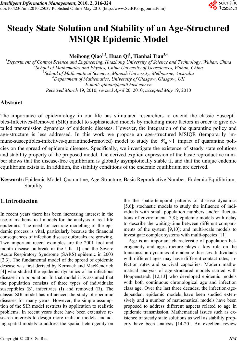Intelligent Information Ma nagement, 2010, 2, 316-324
doi:10.4236/iim.2010.25037 Published Online May 2010 (http://www.SciRP.org/journal/iim)
Steady State Solution and Stability of an Age-Structured
MSIQR Epidemic Model
Meihong Qiao1,2, Huan Qi1, Tianhai Tian3,4
1Department of Control Science and Engineering, Huazho n g Universit y o f Science and Technol o gy, Wuhan, China
2School of Mathematics and Physics, China University of Geosciences, Wuhan, China
3School of Mathematical Sciences, Monash University, Melbourne, Australia
4Department of Mat hem at i cs, University of Gl a sgow, Gl asgow, UK
Received March 19, 2010; revised April 20, 2010; accepted May 19, 2010
Abstract
The importance of epidemiology in our life has stimulated researchers to extend the classic Suscepti-
bles-Infectives-Removed (SIR) model to sophisticated models by including more factors in order to give de-
tailed transmission dynamics of epidemic diseases. However, the integration of the quarantine policy and
age-structure is less addressed. In this work we propose an age-structured MSIQR (temporarily im-
mune-susceptibles-infectives-quarantined-removed) model to study the 01

 impact of quarantine poli-
cies on the spread of epidemic diseases. Specifically, we investigate the existence of steady state solutions
and stability property of the proposed model. The derived explicit expression of the basic reproductive num-
ber shows that the disease-free equilibrium is globally asymptotically stable if, and that the unique endemic
equilibrium exists if. In addition, the stability conditions of the endemic equilibrium are derived.
Keywords: Epidemic Model, Quarantine, Age-Structure, Basic Reproductive Number, Endemic Equilibrium,
Stability
1. Introduction
In recent years there has been increasing interest in the
use of mathematical models for the analysis of real life
epidemics. The need for accurate modelling of the epi-
demic process is vital, particularly because the financial
consequences of infection disease outbreaks are growing.
Two important recent examples are the 2001 foot and
month disease outbreak in the UK [1] and the Severe
Acute Respiratory Syndrome (SARS) epidemic in 2003
[2,3]. The fundamental model of the spread of epidemic
desease was first derived by Kermack and MacKendrick
[4] who studied the epidemic dynamics of an infectious
disease in a population. In that model it is assumed that
the population consists of three types of individuals:
susceptibles (S), infectivies (I) and removed (R). The
classic SIR model has influenced the study of epedimic
diseases for many years. However, the simple assump-
tion of the SIR model restricts its application to realistic
problems. In recent years there have been extensive re-
search interests to design more realistic models, includ-
ing spatial models to address the spatial heterogenity on
the the spatio-temporal patterns of disease dynamics
[5,6]; stochastic models to study the influence of indi-
viduals with small population numbers and/or fluctua-
tions of environment [7,8]; epidemic models with delay
to describe the waiting-time between different compart-
ments of the system [9,10]; and multi-scale models to
investigate complex systems with multi-species [11].
Age is an important characteristic of population het-
erogeneity and age-structure plays a key role on the
transmission dynamics of epidemic diseases. Individuals
with different ages may have different contact rates, in-
fection rates and survival capacities. Modern mathe-
matical analysis of age-structured models started with
Hoppensteadt [12,13] who developed epidemic models
with both continuous chronological age and infection
class age. Over the last three decades, the infection-age-
dependent epidemic models have been studied exten-
sively and a number of mathematical models have been
proposed to address different aspects related to age in
epidemic transmission. Mathematical issues such as ex-
istence of steady state solutio ns as well as stability prop-
erty have been analysis [14-20]. An excellent review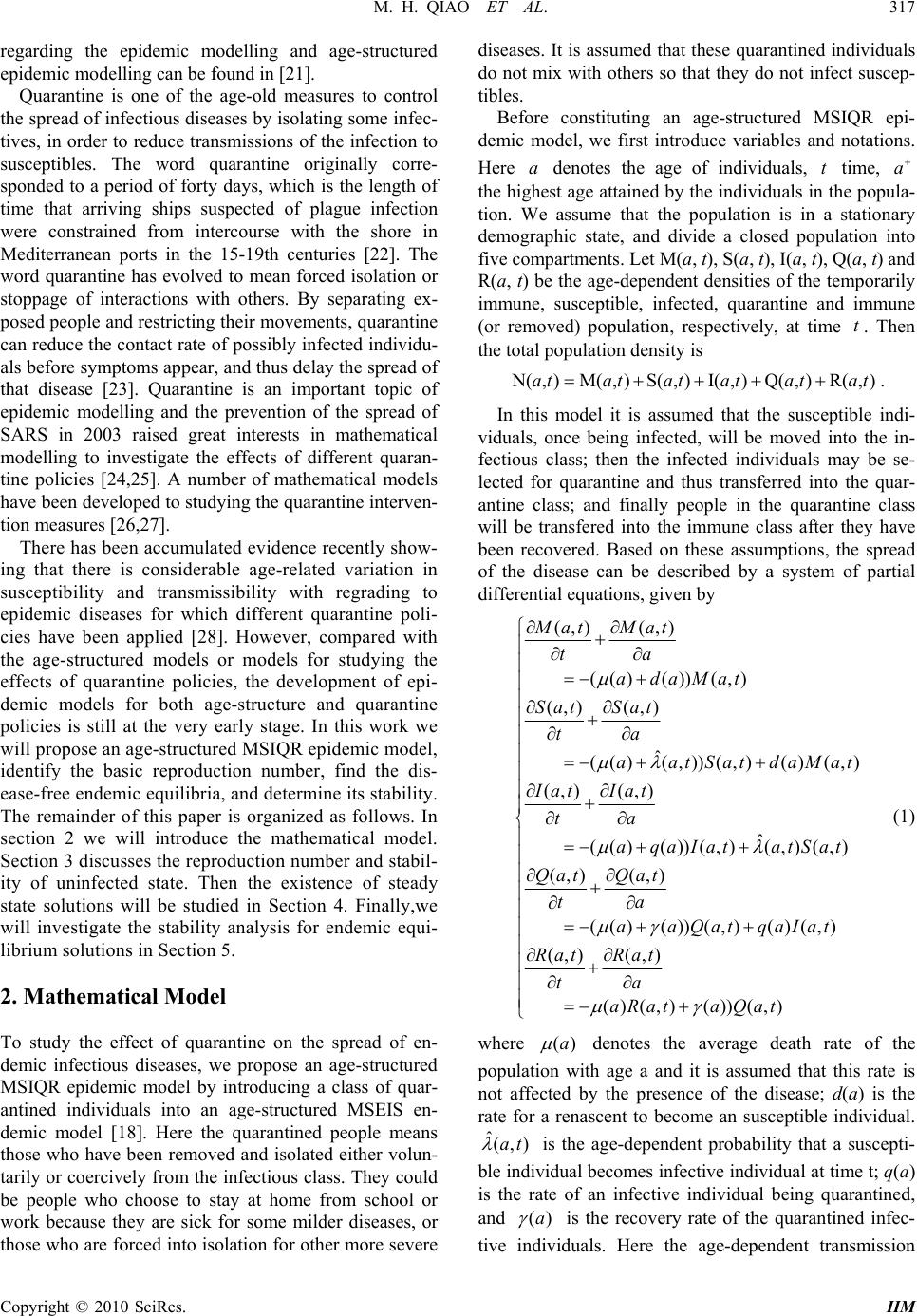

M. H. QIAO ET AL. 317
regarding the epidemic modelling and age-structured
epidemic modelling can be found in [21].
Quarantine is one of the age-old measures to control
the spread of infectious diseases by isolating some infec-
tives, in order to reduce transmissions of the infection to
susceptibles. The word quarantine originally corre-
sponded to a period of forty days, which is the length of
time that arriving ships suspected of plague infection
were constrained from intercourse with the shore in
Mediterranean ports in the 15-19th centuries [22]. The
word quarantine has evolved to mean forced isolation or
stoppage of interactions with others. By separating ex-
posed people and restricting their movements, quarantine
can reduce the contact rate of possibly infected individu-
als before symptoms appear, and thus delay the spread of
that disease [23]. Quarantine is an important topic of
epidemic modelling and the prevention of the spread of
SARS in 2003 raised great interests in mathematical
modelling to investigate the effects of different quaran-
tine policies [24,25]. A number of mathematical models
have been developed to studying th e quaran tine inter ven-
tion measures [26,27].
There has b een accumulat ed evidence r ecently show-
ing that there is considerable age-related variation in
susceptibility and transmissibility with regrading to
epidemic diseases for which different quarantine poli-
cies have been applied [28]. However, compared with
the age-structured models or models for studying the
effects of quarantine policies, the development of epi-
demic models for both age-structure and quarantine
policies is still at the very early stage. In this work we
will propose an age-structured MSIQR epidemic model,
identify the basic reproduction number, find the dis-
ease-free endemic equilibria, and determine its stability.
The remainder of this paper is organized as follows. In
section 2 we will introduce the mathematical model.
Section 3 discusses the reproduction number and stabil-
ity of uninfected state. Then the existence of steady
state solutions will be studied in Section 4. Finally,we
will investigate the stability analysis for endemic equi-
librium solutions in Section 5.
2. Mathematical Model
To study the effect of quarantine on the spread of en-
demic infectious diseases, we propose an age-structured
MSIQR epidemic model by introducing a class of quar-
antined individuals into an age-structured MSEIS en-
demic model [18]. Here the quarantined people means
those who have been removed and isolated either volun-
tarily or coercively from the infectious class. They could
be people who choose to stay at home from school or
work because they are sick for some milder diseases, or
those who are forced into isolation for other more severe
diseases. It is assumed that these quarantined individuals
do not mix with others so that they do not infect suscep-
tibles.
Before constituting an age-structured MSIQR epi-
demic model, we first introduce variables and notations.
Here denotes the age of individuals, t time, aa

the highest age attain ed by the individuals in the popula-
tion. We assume that the population is in a stationary
demographic state, and divide a closed population into
five compartments. Let M(a, t), S(a, t), I(a, t), Q(a, t) and
R(a, t) be the age-dependent densities of the temporarily
immune, susceptible, infected, quarantine and immune
(or removed) population, respectively, at time . Then
the total population density is t
N
(,)M(,)S(,)I(,)Q(,)R(,)atatat atatat

 .
In this model it is assumed that the susceptible indi-
viduals, once being infected, will be moved into the in-
fectious class; then the infected individuals may be se-
lected for quarantine and thus transferred into the quar-
antine class; and finally people in the quarantine class
will be transfered into the immune class after they have
been recovered. Based on these assumptions, the spread
of the disease can be described by a system of partial
differential equations, given by
(,) (,)
(()()) (,)
(,) (,)
ˆ
(()(,))(,)() (,)
(,) (,)
ˆ
(() ())(,)(,)(,)
(,) (,)
(() ())(,)()(,)
(,)
MatMat
ta
adaMat
Sat Sat
ta
aatSatdaMa
Iat Iat
ta
aqa IatatSat
Qat Qat
ta
aaQatqaIat
Rat
t







 



 



 



 


t
(,)
()(,)()) (,)
Rat
a
aRata Qat 





















 

(1)
where ()a

denotes the average death rate of the
population with age a and it is assumed that this rate is
not affected by the presence of the disease; d(a) is the
rate for a renascent to become an susceptible individual.
is the age-dependent probability that a suscepti-
ble individual becomes infective individual at time t; q(a)
is the rate of an infective individual being quarantined,
and
ˆ(,)at

()a

is the recovery rate of the quarantined infec-
tive individuals. Here the age-dependent transmission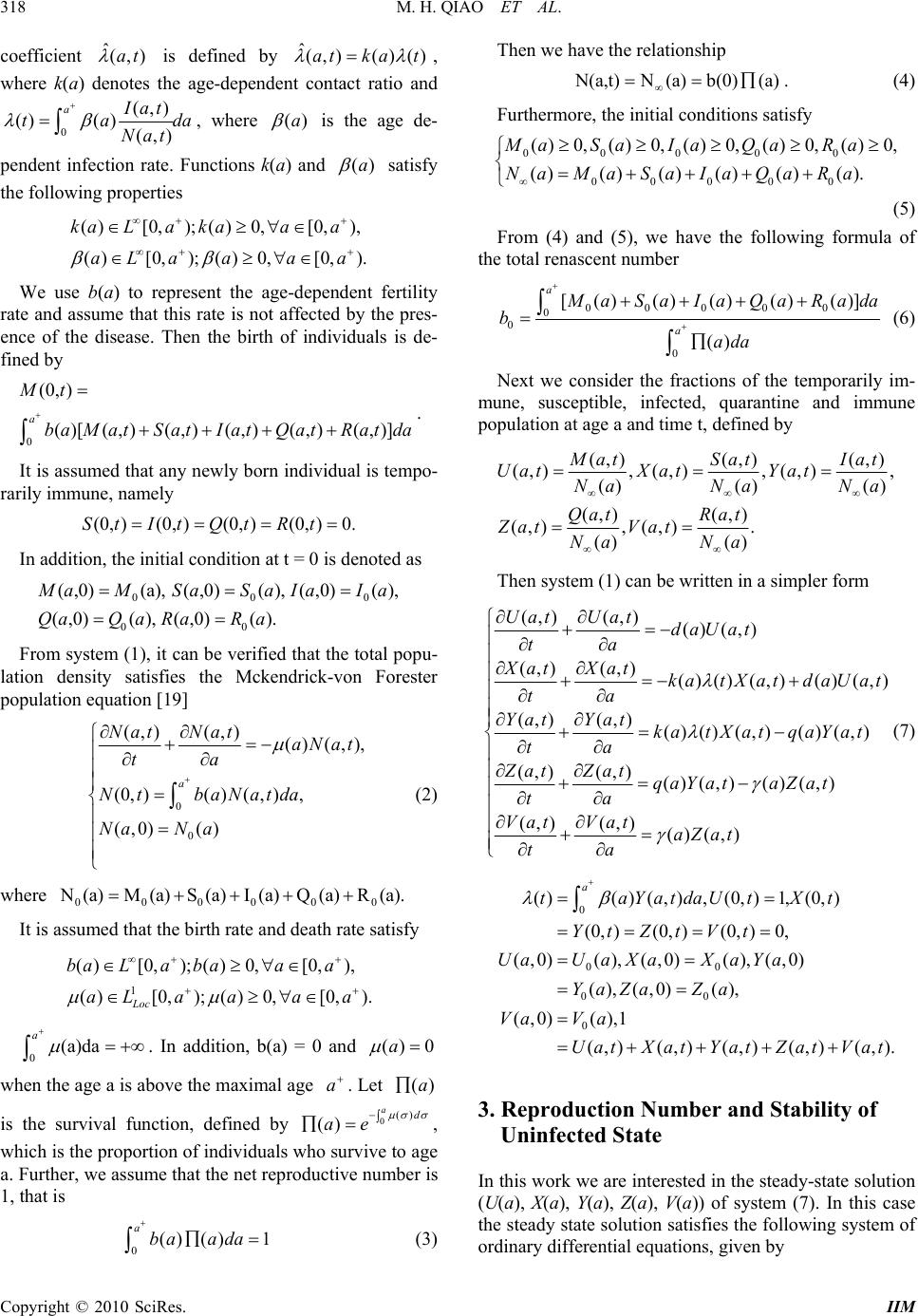

318 M. H. QIAO ET AL.
coefficient is defined by
ˆ(,)at

ˆ(,) ()()atka t

 ,
where k(a) denotes the age-dependent contact ratio and
0
(,
( )(,
Ia
ta
Na
)
() )
atda
t


, where ()a

is the age de-
pendent infection rate. Functions k(a) and ()a

satisfy
the following properties
() [
() [
L
aL
(,)M at
(0,)St
) (
) ()
0,);() 0
0,); ()
kaa ka
a a





,
0,
Q
()
).
[0, ),
[0,).
a a
a a




(,) (,)]atRatda
(0,) 0.Rt 
0
, (,0)(),
We use b(a) to represent the age-dependent fertility
rate and assume that this rate is not affected by the pres-
ence of the disease. Then the birth of individuals is de-
fined by
0
(0, )
( )[( ,)(,)
a
Mt
baS atIat



.
It is assumed that any newly born individual is tempo-
rarily immune, namely
(0,) (0,)It Qt
In addition, the initial co ndition at t = 0 is denoted as
00
00
(,0a), (,0)
(,0, (,0)(
M
aM
Q a
Sa
QaRa R


S
a
aIaIa
From system (1), it can be verified that the total popu-
lation density satisfies the Mckendrick-von Forester
populat i on eq u a t i on [1 9]
0
0
(,
(0, )
(,0
Nat
Nt
Na









00
) (,)
( )(
) ()
a
Nat
ta
baN
N a







() (,),
,
aNat
da

00
, )at

0
(2)
where 0
N
(a) M
1
() [0
() Loc
L
aL
a
(a)S (a)I (a)

,
0,
a
Q (a)R(a).

[0, ),
[0,).
a
a a




() 0a
It is assumed that the birth rate and dea th rate satisfy
,);() 0
[0,);()
baa ba
a a 



0(a)d
a


. In addition, b(a) = 0 and


when the age a is above the maximal age . Let
a(a)

is the survival function, defined by 0()
() ad ae

 
 ,
which is the proportion of individuals who survive to age
a. Further, we assume that the net reproductive number is
1, that is
0() ()ba ada1
a
 (3)
Then we have the relati onship
N
(a,t)N (a)b(0)(a)


. (4)
Furthermore, the initial conditions satisfy
000 00
000 00
() 0,() 0,()0,() 0,() 0,
()()()()()().
Ma Sa IaQa Ra
NaMaSa IaQaRa





(5)
From (4) and (5), we have the following formula of
the total renascent nu mber
000 00
0
0
0
[()() ()()()]
()
a
a
M
aSaIaQaRada
bada






 (6)
Next we consider the fractions of the temporarily im-
mune, susceptible, infected, quarantine and immune
population at age a and time t, defined by
(,)(,) (,)
(,),(,) ,(,) ,
()() ()
(,) (,)
(,), (,).
() ()
M
atSat Iat
UatXat Yat
NaNaNa
Qat Rat
Zat Vat
Na Na





Then system (1) can be written in a simpler form
(,)(,) () (,)
(,)(,)()()(,)() (,)
(,)(,)()() (,)()(,)
(,)(,) ()(,) ()(,)
(,)(,)()(,)
Uat UatdaUat
ta
Xat Xatka tXat daUat
ta
YatYat katXat qaYat
ta
ZatZatqaYat aZat
ta
VatVataZat
ta








 


 















(7)
0
00
00
0
()()(, ),(0, )1,(0, )
(0, )(0, )(0, )0,
(,0)(),(,0)(),(,0)
(), (,0)(),
(,0) (),1
(,)(,) (,)(,)(,).
a
taYatdaUtXt
YtZtVt
UaUaXaXa Ya
YaZa Za
VaVa
UatXat YatZat Vat









3. Reproduction Number and Stability of
Uninfected State
In this work we are interested in th e steady-state solution
(U(a), X(a), Y(a), Z(a), V(a)) of system (7). In this case
the steady state solution satisfies the fo llowing system of
ordinary differential equations, given by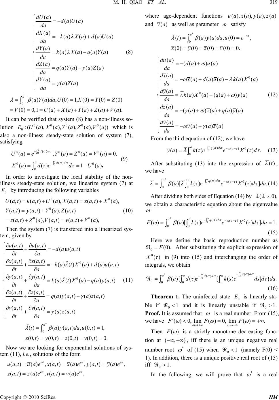

M. H. QIAO ET AL. 319
() ()()
() ()()()()
() ()() ()()
() ()() ()()
() ()( )
dU adaUa
da
dX aka XadaUa
da
dY aka XaqaYa
da
dZ aqaYa aZa
da
dV aaZa
da



















(8)
0()(),(0)1, (0)(0)(0)
(0) 0,1()()()()().
aaYadaUX YZ
VUaXaYaZaV





a

0

0
It can be verified that system (8) has a non-illness so-
lution which is
also a non-illness steady-state solution of system (7),
satisfying
00000
0:( (),(), (),(),())EUaXaYaZaVa
0
0
()
0000
()
0
0
(),()()() 0.
()()1 ()
add
add
UaeYaZa Va
Xad edUa










，
(9)
In order to investigate the local stability of the non-
illness steady-state solution, we linearize system (7) at
by introducing the following variables
0
E
0
0
00
(,)(,)(),(,)(,)(),
(,)(,)(),(,)
(,)(), (,)(,)(),
UatuatUaX atxatXa
YatyatYaZat
zatZaVatvatVa
 

 
(10)
Then the system (7) is transfered into a linearized sys-
tem, given by
0
0
(,) (,)()(,)
(,)(,)()() ()()(,)
(,)(,) ()() ()()(,)
(,)(,) ()(,) ()(,)
(,)(,) ()(,)
uat uatdauat
ta
xat xatkatX adauat
ta
yatyat katX aqayat
ta
zatzat qayatazat
ta
vat vatazat
ta








 


 


 














(11)
0
()( )( ,),(0,)1,
(0,)(0, )(0, )(0, )0.
a
tayatdaut
xtytzt vt






Now we are looking for exponential solutions of sys-
tem (11), i.e., solutions of the form
(,)(),(,)(),(,)()
(,)(),(,)(),
tt
tt
uatuae xatxaeyatyae
zatzae vatvae
where age-dependent functions (),(), (),()ua xaya za
and ()va as well as parameter

satisfy
0
()()(),(0),
(0)(0)(0)(0) 0.
at
tayadaue
xyzv






0
0
() (() )()
() ()()()() ()
() ()() (())()
() (())()()()
() () ()()
du ada ua
da
dx a
x
adaua kaXa
da
dy akaXaqaya
da
dz aazaqaya
da
dv avaaza
da





 


 








 


(12)
From the third equation of (12), we have
() ()0
0
()()() .
a
aqd a
y
akeeX

 
d




  (13)
After substituting (13) into the expression of )(t

,
we have
() ()0
00
()[()()] .
a
aa
qd a
akee Xdd

 
 


 a (14)
After dividing both sides of Equation (14) by (0)  ,

we obtain a characteristic equation about the eigenvalue

() ()0
00
()()[()() ]1.
a
aaqd a
FakeeXdd

 
 

a



(15)
Here we define the basic reproduction number as
0(0).F


0()X
After substituting the explicit expression of

in (9) into (15) and interchanging the order of
integrals, we obtain
0()
()
000
(){()[()]} .
a
sqd
aa a
dd
adeksedsdda



 




 
(16)
Theorem 1. The uninfected state is linearly sta-
ble if 0
E
01

 and it is linearly unstable if 01.


Proof. It is assumed that

is a real number. From (15),
we have ()0,lim) 0,l()F

(FFim.


 



,
t





Then ()F

is a strictly monotone decreasing func-
tion at (,)


*
, iff there is an unique negative real
number root

of (15) when (namely F(0) <
1). In addition, there is a unique positive real root of (15)
iff
01
01.


In the following, we will prove that *

is a real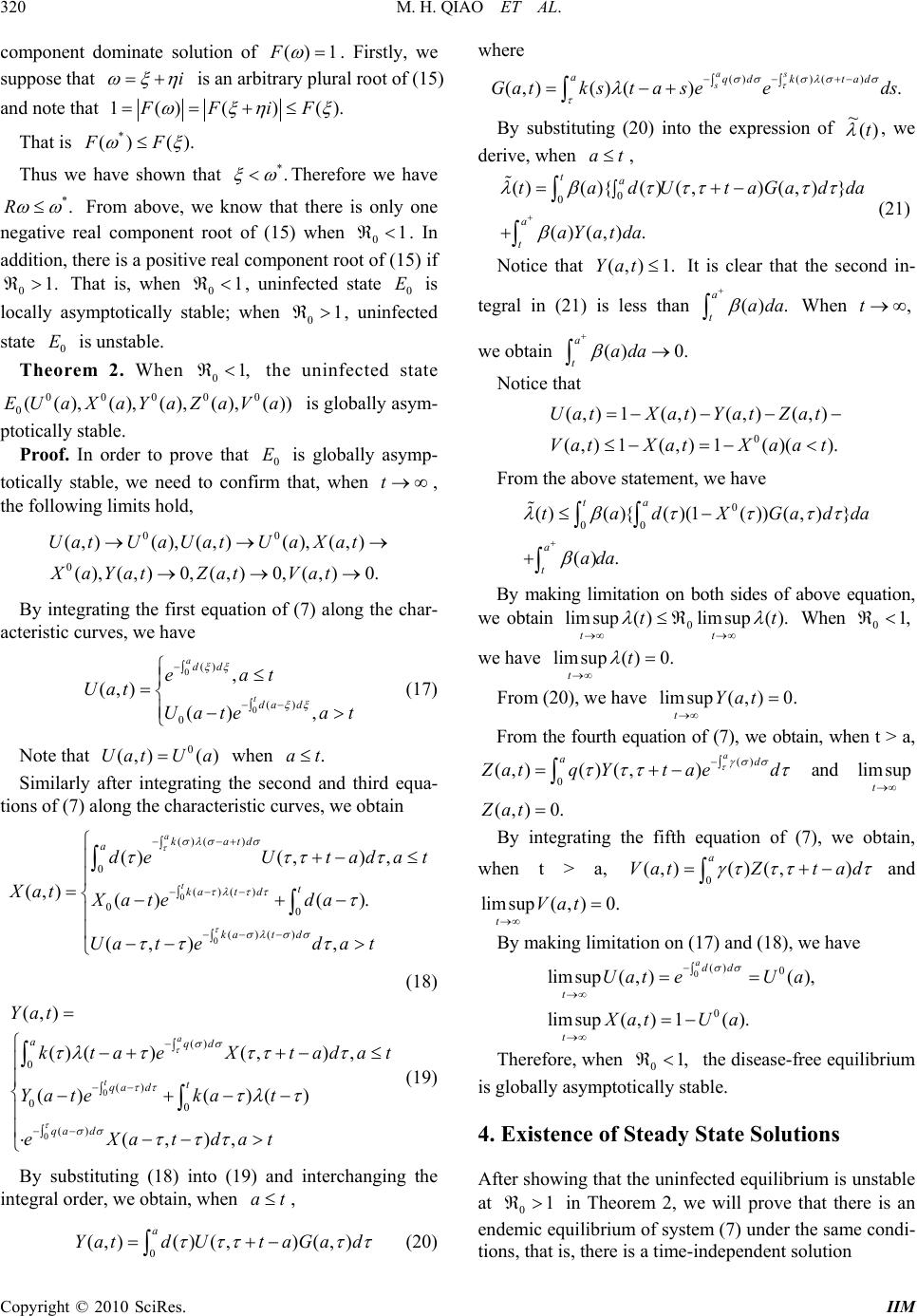

320 M. H. QIAO ET AL.
component dominate solution of () 1F

. Firstly, we
suppose that i

  is an arbitrary plur al root of (15)
and note that 1() ().FF)(iF

 
.
 
That is * () ()FF

 
Thus we have shown that *.

 Therefore we have
*.R

 
01.
0
E
From above, we know that there is only one
negative real component root of (15) when . In
addition, there is a positive real component root of (15) if
That is, when , uninfected state is
locally asymptotically stable; when , uninfected
state is unstable.
01
0
E
0
1
01
Theorem 2. When the uninfected state
is globally asym-
01,
0
( ),Z aV
0000
0(( ),( ),( ),( ))EU aXaY aa
ptotically stable.
Proof. In order to prove that is globally asymp-
totically stable, we need to confirm that, when ,
the following limits hold,
0
E
t
00
0
(,)(),(,)(),(,)
(),(,) 0,(,) 0,(,)0.
UatU aUatUaXat
XaYatZat Vat




t
By integrating the first equation of (7) along the char-
acteristic curves, we have
0
0
()
()
0
,
(,) () ,
a
t
dd
dad
eat
Uat Uateat











(17)
Note that when
0
(,) ()UatU a.at
Similarly after integrating the second and third equa-
tions of (7) along the characteristic curves, we obtain
0
0
()()
0
()()
00
()()
()(,),
(,) ()( ).
(,) ,
a
t
katd
a
t
katd
katd
deU tadat
Xat Xateda
Uated at


 
 
 


 






 




 



(18)
0
0
()
0
()
00
()
(,)
()()(,) ,
()()()
(,),
a
t
aqd
t
qad
qa d
Yat
ktaeX tada
Yatekat
eXatdat





 
 








 







 (19)
By substituting (18) into (19) and interchanging the
integral order, we obtain, when , at
0
(,)() (,) (,)
a
YatdUt aGad

  
 (20)
where
()()()
(,)()().
as
s
aqd ktad
Gatkstaseeds

 






By substituting (20) into the expression of )(
~
t 
, we
derive, when at

,
0
0
()(){()(,)(,)}
()(,) .
ta
a
t
tadUtaGad
aYatda
 







da
(21)
Notice that (,) 1.Yat

It is clear that the second in-
tegral in (21) is less than When
we obtain
() .
a
tada


,t
() 0ada  .
a
t


Notice that
0
(,) 1(,)(,)(,)
(,)1(,) 1()().
UatXat YatZat
VatXatXa at




da
From the above statement, we have
0
00
()(){()(1( ))( ,)}
() .
ta
a
t
tadXGad
ada
 







By making limitation on both sides of above equation,
we obtain 0 limsup()limsup().
tt
tt


 

 When 01,


we have limsup()0.
tt



From (20), we have limsup(, )0.
tYat 

From the fourth equation of (7), we obtain, when t > a,
()
0
(,)()(,) a
ad
Z
atqYt aed

 

 



(,)0.Zat
and limsup
t

By integrating the fifth equation of (7), we obtain,
when t > a, 0
(,) ()(,)
a
VatZt ad

  
and
limsup(, )0.
tVat 

By making limitation on (17) and (18), we have
0() 0
0
limsup(, )(),
limsup(, )1().
add
t
t
UateUa
XatUa
 





Therefore, when 01,

 the disease-free equilibrium
is globally asymptotically stable.
4. Existence of Steady State Solutions
After showing that the uninfected equilibrium is unstable
at 01

 in Theorem 2, we will prove that there is an
endemic equilibrium of system (7) under the same condi-
tions, that is, there is a time-independent solution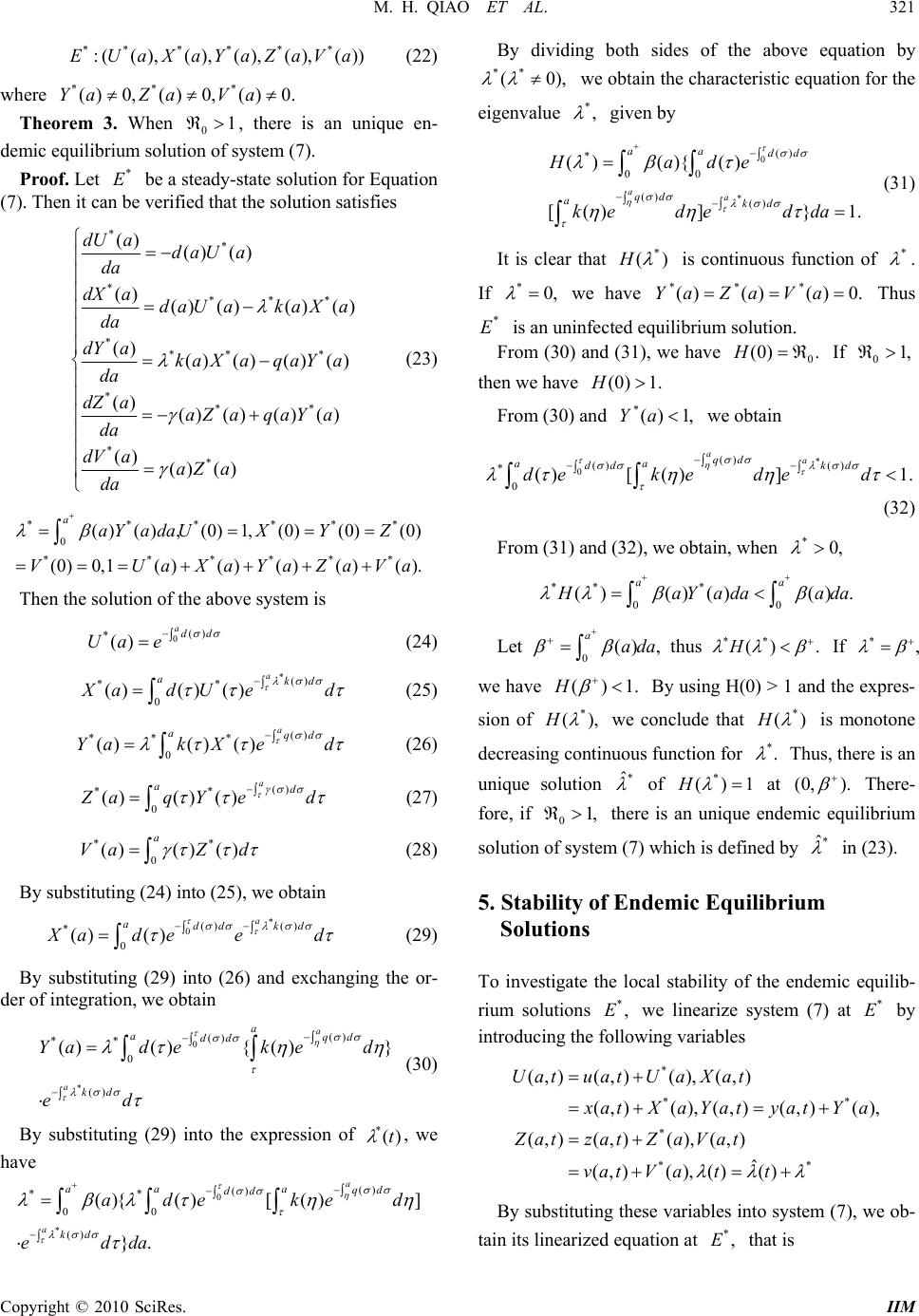

M. H. QIAO ET AL. 321

*** ** *
:( (),(), (),(), ())EUaXaYaZaVa
(22)
where
***
() 0,() 0,() 0.YaZaVa
Theorem 3. When , there is an unique en-
demic equilibrium solution of system (7).
01
Proof. Let be a steady-state solution for Equation
(7). Then it can be verified that the solution satisfies
*
E
**
****
*** *
***
**
() () ()
() () ()()()
() ()()() ()
() ()()()()
() ()()
dU adaU a
da
dX adaU akaXa
da
dY akaXaqaY a
da
dZ aaZaqaY a
da
dV aaZa
da













 





(23)
*****
0
*****
()(),(0) 1,(0)(0)(0)
(0) 0,1()()()()().
aaY adaUXYZ
VUaXaYaZaV




*
*
a

Then the solution of the above system is
0()
*()add
Ua e

 
 (24)
*()
**
0
()() ()a
akd
X
adUed





  (25)
()
** *
0
()()()a
aqd
Yak Xed





  (26)
()
**
0
()()()a
ad
Z
aqYe d

 



  (27)
**
0
()() ()
a
VaZ d

   (28)
By substituting (24) into (25), we obtain
*
0() ()
*
0
() ()a
add kd
X
ade ed


 




 (29)
By substituting (29) into (26) and exchanging the or-
der of integration, we obtain
0
*
()
()
**
0
()
()(){ ()}
a
a
a
aqd
dd
kd
Yad eked
ed



















(30)
By substituting (29) into the expression of , we
have
)(
*t

0
*
()
()
**
00
()
(){()[ ()]
}.
a
a
aa a
qd
dd
kd
adeke d
edda







 









 
By dividing both sides of the above equation by
we obtain the characteristic equation for the
eigenvalue
**
(0  ),
*,

given by
0
*
()
*
00
() ()
()(){ ()
[()]} 1
aa
aadd
qd
akd
Hade
k ededda



 


 





.



(31)
It is clear that * ()H

is continuous function of *

.
If *0, 

we have Thus
is an uninfected equilibrium solution.
***
()()() 0.YaZa Va
*
EFrom (30) and (31), we have If
0
(0) .H 01,


then we have (0) 1.H
From (30) and *() 1,Ya

we obtain
*
0()
() ()
*
0()[ ()]1.
aa
qd
aa
dd kd
deke ded


 








(32)
From (31) and (3 2) , we obtain , when
*0,
 
** *
00
()() ()() .
aa
H
aY adaada  



Let thus
0() ,
aada


**
() .H



 If *




,
we have ()1.H



By using H(0) > 1 and the expres-
sion of * (),H

we conclude that * ()H

is monotone
decreasing continuous function for *.

Thus, there is an
unique solution *
ˆ

of at
*
()1  (0,H).

 There-
fore, if 01,

 there is an unique endemic equilibrium
solution of system (7) which is defined by *
ˆ

in (23).
5. Stability of Endemic Equ il ib ri um
Solutions
To investigate the local stability of the endemic equilib-
rium solutions we linearize system (7) at by
introducing the following variables
*,E*
E
*
**
*
**
(,)(,)(), (,)
(,)(), (,)(,)(),
(,)(,)(), (,)
ˆ
( ,)(),()()
UatuatUa Xat
x
atXaYatyatYa
ZatzatZ aVat
vatV att 

 

 
By substituting these variables into system (7), we ob-
tain its linearized equation at that is
*,E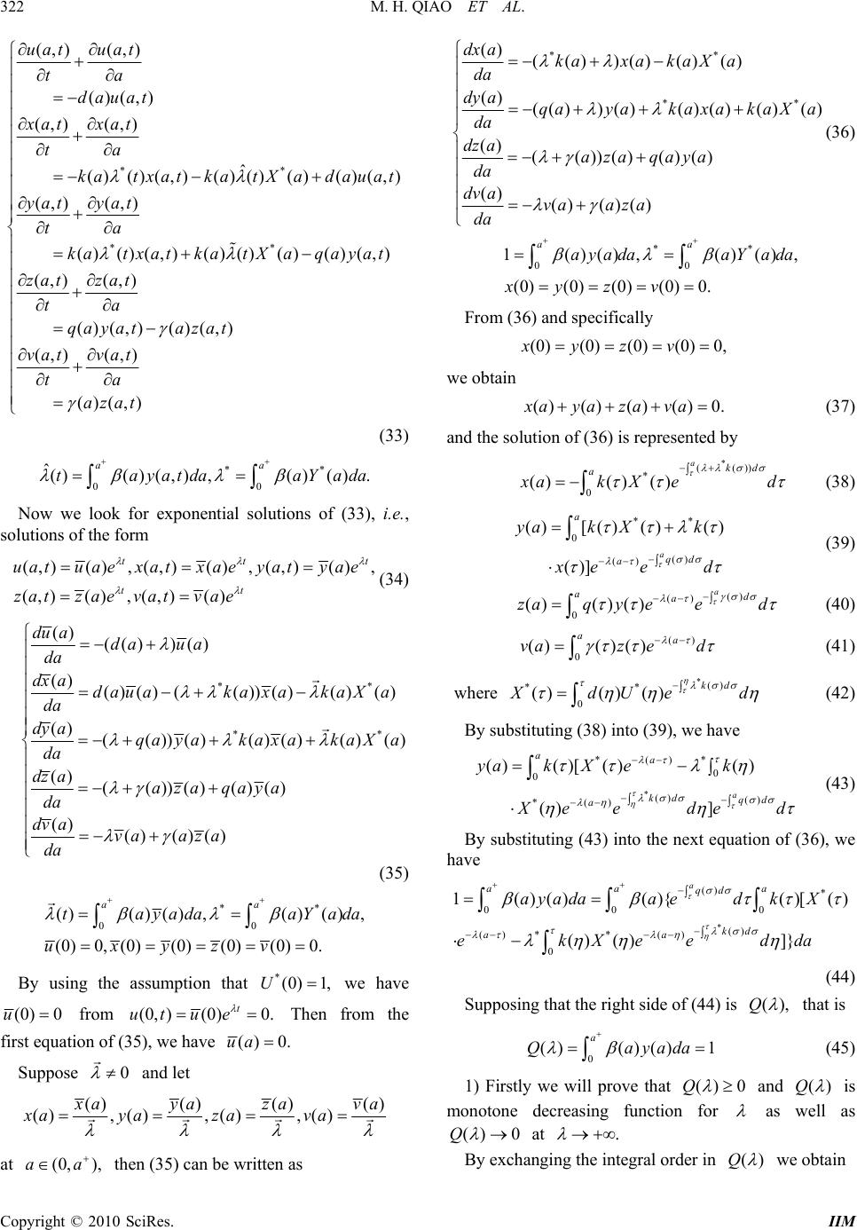

322 M. H. QIAO ET AL.
**
**
(,) (,)
()(,)
(,) (,)
ˆ
() ()(,)()()()()(,)
(,)(,)
() ()(,)()()()()(,)
(,)(,)
()(,)()(,)
(,
uat uat
ta
dauat
xat xat
ta
katxatkatXadauat
yat yat
ta
katxatkatXaqayat
zat zat
ta
qayat azat
va










 










)(,)
()(,)
tvat
ta
azat 
























(33)
**
00
ˆ()()(,) ,() ().
aa
tayatda aYa  



da
Now we look for exponential solutions of (33), i.e.,
solutions of the form
(,)() ,(,)() ,(,)() ,
(,)() ,(,)()
tt
tt
uatuae xatxae yatyae
zatzae vatvae
t




 (34)
**
*
() (() )()
() ()() (())()()()
() (())()()()() ()
() (())()()()
() () ()()
du ada ua
da
dx adauakaxakaXa
da
dy aqa yakaxakaXa
da
dz aaza qaya
da
dv ava aza
da

 



 


 








 



*
(35)
**
00
()( )( ),( )(),
(0) 0,(0)(0)(0)(0) 0.
aa
tayadaaYa
uxyzv
 




da
By using the assumption that we have
*(0) 1,U
(0) 0u from (0,)(0)0.
t
ut ue

 Then from the
first equation of (35), we have () 0.ua
Suppose and let
0  

()()() ()
() ,(),() ,()
x
ayazav
xayazava a






at then (35) can be written as (0, ),aa


**
**
() (())()()()
() (())()()()()()
() (())() ()()
() () ()()
dx akaxakaX a
da
dy aqayakaxakaX a
da
dz aaza qaya
da
dv ava aza
da




 


 







(36)
**
00
1()() ,()(),
(0)(0)(0)(0) 0.
aa
ayadaaY ada
xyzv






From (36) and specifically
(0)(0)(0)(0)0, xyzv


we obtain
()()()() 0.xayaza va

 (37)
and the solution of (36) is represented by
*
(())
*
0
()()()
akd
a
x
akXe

 
d





 (38)
**
0
()
()
()[() ()()
()] a
a
qd
a
yak Xk
x
ee d








 


 (39)
()
()
0
() ()()a
ad
a
zaqy eed

 




 
 (40)
()
0
() ()()
aa
vaz ed


 

 (41)
where *()
**
0
()() ()kd
X
dU ed






  (42)
By substituting (38) into (39), we have
*
*()*
0
0
() ()
*()
()()[ ()()
()] a
aa
kd qd
a
yak Xek
X
eede d






 




 



 (43)
By substituting (43) into the next eq uation of (36), we
have
*
() *
00 0
()
() **()
0
1()() (){()[
() ()]}
a
aa a
qd
kd
aa
ayadaa edkX
ekXeedda





 
()











 


(44)
Supposing that the right side of (44) is (),Q

that is
0
()()()1
a
Qayad 
a


 (45)
1) Firstly we will prove that ()0Q

 and ()Q

is
monotone decreasing function for

as well as
() 0Q

 at .


By exchanging the integral order in ()Q

we obtain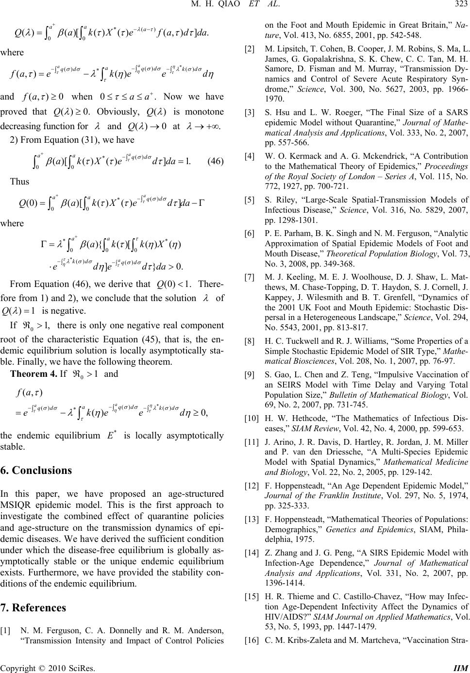

M. H. QIAO ET AL. 323
da
*()
00
()()[()()(,)] .
aa a
QakXefad

 


where
*
()
() ()
*
(,)() a
aaqd
qd kd
f
aeke ed




 





 






and (,)0fa


Q
when Now we have
proved that
0aa 

 .
() 0.

 Obviously, (Q)

is monotone
decreasing function for

and ()Q0

 at .


2) From Equation (31), we have
()
*
00
()[() ()]1.
a
aa qd
akXedda




 (46)
Thus
()
*
00
(0)()[( )( )]
a
aa qd
QakXedd


 


 a
*
0.
where
*
*
000
() ()
(){()[() ()
]}
a
aa
kd qd
ak kX
ededda















From Equation (46), we derive that There-
fore from 1) and 2), we conclude that the solution
(0)1.Q

of
() 1Q

 is negative.
If there is only one negative real component
root of the characteristic Equation (45), that is, the en-
demic equilibrium solution is locally asymptotically sta-
ble. Finally, we have the following theorem.
01,
Theorem 4. If and
01
*
()
() ()
*
(, )
() 0,
a
aaqd
qd kd
fa
ekeed




 


 






the endemic equilibrium is locally asymptotically
stable.
*
E
6. Conclusions
In this paper, we have proposed an age-structured
MSIQR epidemic model. This is the first approach to
investigate the combined effect of quarantine policies
and age-structure on the transmission dynamics of epi-
demic diseases. We have derived the sufficient condition
under which the disease-free equilibrium is globally as-
ymptotically stable or the unique endemic equilibrium
exists. Furthermore, we have provided the stability con-
ditions of the end e mic equilibrium.
7
. References
[1] N. M. Ferguson, C. A. Donnelly and R. M. Anderson,
“Transmission Intensity and Impact of Control Policies
on the Foot and Mouth Epidemic in Great Britain,” Na-
ture, Vol. 413, No. 6855, 2001, pp. 542-548.
[2] M. Lipsitch, T. Cohen, B. Cooper, J. M. Robins, S. Ma, L.
James, G. Gopalakrishna, S. K. Chew, C. C. Tan, M. H.
Samore, D. Fisman and M. Murray, “Transmission Dy-
namics and Control of Severe Acute Respiratory Syn-
drome,” Science, Vol. 300, No. 5627, 2003, pp. 1966-
1970.
[3] S. Hsu and L. W. Roeger, “The Final Size of a SARS
epidemic Model without Quarantine,” Journal of Mathe-
matical Analysis and Applications, Vol. 333, No. 2, 2007,
pp. 557-566.
[4] W. O. Kermack and A. G. Mckendrick, “A Contribution
to the Mathematical Theory of Epidemics,” Proceedings
of the Royal Society of London – Series A, Vol. 115, No.
772, 1927, pp. 700-721.
[5] S. Riley, “Large-Scale Spatial-Transmission Models of
Infectious Disease,” Science, Vol. 316, No. 5829, 2007,
pp. 1298-1301.
[6] P. E. Parham, B. K. Singh and N. M. Ferguson, “Analytic
Approximation of Spatial Epidemic Models of Foot and
Mouth Disease,” Theoretical Population Biology, Vol. 73,
No. 3, 2008, pp. 349-368.
[7] M. J. Keeling, M. E. J. Woolhouse, D. J. Shaw, L. Mat-
thews, M. Chase-Topping, D. T. Haydon, S. J. Cornell, J.
Kappey, J. Wilesmith and B. T. Grenfell, “Dynamics of
the 2001 UK Foot and Mouth Epidemic: Stochastic Dis-
persal in a Heterogeneous Landscape,” Science, Vol. 294,
No. 5543, 2001, pp. 813-817.
[8] H. C. Tuckwell and R. J. Williams, “Some Properties of a
Simple Stochastic Epidemic Model of SIR Type,” Mathe-
matical Biosciences, Vol. 208, No. 1, 2007, pp. 76-97.
[9] S. Gao, L. Chen and Z. Teng, “Impulsive Vaccination of
an SEIRS Model with Time Delay and Varying Total
Population Size,” Bulletin of Mathematical Biology, Vol.
69, No. 2, 2007, pp. 731-745.
[10] H. W. Hethcode, “The Mathematics of Infectious Dis-
eases,” SIAM Review, Vol. 42, No. 4, 2000, pp. 599-653.
[11] J. Arino, J. R. Davis, D. Hartley, R. Jordan, J. M. Miller
and P. van den Driessche, “A Multi-Species Epidemic
Model with Spatial Dynamics,” Mathematical Medicine
and Biology, Vol. 22, No. 2, 2005, pp. 129-142.
[12] F. Hoppensteadt, “An Age Dependent Epidemic Model,”
Journal of the Franklin Institute, Vol. 297, No. 5, 1974,
pp. 325-333.
[13] F. Hoppensteadt, “Mathematical Theories of Populations:
Demographics,” Genetics and Epidemics, SIAM, Phila-
delphia, 1975.
[14] Z. Zhang and J. G. Peng, “A SIRS Epidemic Model with
Infection-Age Dependence,” Journal of Mathematical
Analysis and Applications, Vol. 331, No. 2, 2007, pp.
1396-1414.
[15] H. R. Thieme and C. Castillo-Chavez, “How may Infec-
tion Age-Dependent Infectivity Affect the Dynamics of
HIV/AIDS?” SIAM Journal on Applied Mathematics, Vol.
53, No. 5, 1993, pp. 1447-1479.
[16] C. M. Kribs-Zaleta and M. Martcheva, “Vaccination Stra-

324 M. H. QIAO ET AL.
tegies and backward Bifurcation in an Age-since-Infection
Structured Model,” Mathematical Biosciences, Vol. 177-
178, 2002, pp. 317-332.
[17] H. Inaba and H. Sekine, “A Mathematical Model for Cha-
gas Disease with Infection-Age-Dependent Infectivity,”
Mathematical Biosciences, Vol. 190, No. 1, 2004, pp. 39-
69.
[18] B. Fang and X. Li, “Stability of an Age-Structured
MSEIS Epidemic Model with Infectivity in Latent Pe-
riod,” Acta Mathematicae Applicatae Sinica, Vol. 31, No.
1, 2008, pp. 110-125.
[19] G. B. Webb, “Theory of Nonlinear Age-Dependent Popu-
lation Dynamics,” CRC Press, Boca Raton, 1985.
[20] J. Li, Y. C. Zhou, Z. Z. Ma and M. Hyman, “Epidemiol-
ogical Models for Mutating Pathogens,” SIAM Journal on
Applied Mathematics, Vol. 65, No. 1, 2004, pp. 1-23.
[21] H. W. Hethcotevan and P. den Driessche, “Two SIS Epi-
demiologic Models with Delay s,” Journal of Mathematical
Biology, Vol. 40, No. 1, 2000, pp. 3-26.
[22] W. H. McNeill, “Plagues and Peoples,” Updated Edition,
Anchor, Garden City, 1976.
[23] A. Mandavilli, “SARS Epidemic Unmasks Age-Old
Quarantine Conundrum,” Nature Medicine, Vol. 9, No. 5,
2003, p. 487.
[24] B. Diamond, “SARS Spreads New Outlook on Quaran-
tine Models,” Nature Medicine, Vol. 9, No. 12, 2003, p.
1441.
[25] Y. H. Hsieh, C. C. King, C. W. Chen, M. S. Ho, S. B.
Hsu and Y. C. Wu, “Impact of Quarantine on the 2003
SARS Outbreak: A Retrospective Modeling Study,” Jour-
nal of Theoretical Biology, Vol. 244, No. 4, 2007, pp.
729-736.
[26] L. Sattenspiel and D. A. Herring, “Simulating the Effect
of Quarantine on the Spread of the 1918-19 Flu in Central
Canada,” Bulletin of Mathematical Biology, Vol. 65, No.
1, 2003, pp. 1-26.
[27] H. W. Hethcote, Z. E. Ma and S. B. Liao, “Effects of
Quarantine in Six Endemic Models for Infectious Dis-
eases,” Mathematical Biosciences, Vol. 180, No. 1, 2002,
pp. 141-160.
[28] C. T. Bauch, J. O. Lloyd-Smith, M. P. Coffee and A. P.
Galvani, “Dynamically Modelling SARS and Other Newly
Emerging Respiratory Illnesses: Past, Present and Fu-
ture,” Epidemiology, Vol. 16, No. 6, 2005, pp. 791-801.