Open Journal of Statistics, 2012, 2, 208-212
http://dx.doi.org/10.4236/ojs.2012.22025 Published Online April 2012 (http://www.SciRP.org/journal/ojs)
Stochastic Orders Comparisons of Negative Binomial
Distribution with Negative Binomial—Lindley Distribution
Chookait Pudprommarat, Winai Bodhisuwan
Department of Statistics, Kasetsart University, Bangkok, Thailand
Received January 20, 2012; revised February 18, 2012; accepted March 4, 2012
ABSTRACT
The purpose of this study is to compare a negative binomial distribution with a negative binomial—Lindley by using
stochastic orders. We characterize the comparisons in usual stochastic order, likelihood ratio order, convex order, ex-
pectation order and uniformly more variable order based on theorem and some numerical example of comparisons be-
tween negative binomial random variable and negative binomial—Lindley random variable.
Keywords: Stochastic Orders; Negative Binomial Distribution; Negative Binomial—Lindley Distribution
1. Introduction



 


The negative binomial (NB) distribution is a mixture of
Poisson distribution by mixing the Poisson distribution
and gamma distribution. The NB distribution is em-
ployed as a functional form that relaxes the overdisper-
sion (variance is greater than the mean) restriction of the
Poisson distribution (see [1]). If X denote a random
variable of NB distributed with parameter r and p then its
probability mass function is in form

rx
fx 
 
x
r
1
p 1 p



x

0p1
, , x0,1,2,
 
for and , with r0r1 p
EX
p

 and
 
2
r1
Xp

p Var .
The negative binomial—Lindley (NB-L) distribution
which is a mixed negative binomial distribution obtained
by mixing the negative binomial distribution with a Lind-
ley distribution. The NB-L distribution was introduced
by Zamani and Ismail in [2] and it provides a model for
count data of insurance claims. If Y is a NB-L random
variable with parameter r and

then its probability
mass function is in form
 

2
yj
ry1 y
gy 1




2
j0
rj1
yj rj

 



r 0
,
y0,1,2,, for and

, with
 
3
r
11

  1
2rEY , when



, and



22 23
22
2
2
23
2
24
rr1 2rr
Var Y
12 11
r11
r,
11


 
 

 

 
 


2 when 

.

In this respect, the aim of this work is to compare a
negative binomial distribution with negative binomial—
Lindley distribution base on stochastic orders such as
usual stochastic order, likelihood ratio order, convex or-
der, expectation order and uniformly more variable order.
2. Stochastic Orders
Stochastic orders are useful in comparing random vari-
ables measuring certain characteristics in many areas.
Such areas include insurance, operations research, queu-
ing theory, survival analysis and reliability theory (see
[3]). The simplest comparison is through comparing the
expected value of the two comparable random variables.
The following, we will define some notions of the sto-
chastic orders which will be used in the context of the
paper. For more details, we refer to Ross [4], Misra [5],
Shaked [6,7] and Singh [8].
Definition 1. Let X and Y be random variables with
densities f and g, respectively, such that


gkf k is
non-decreasing function in k over the union of the sup-
ports of X and Y, or, equivalently,








fugvfvguuv
lr
XY
, for all . Then X is smaller
than Y in the likelihood ratio order which is denoted by

.
C
opyright © 2012 SciRes. OJS

C. PUDPROMMARAT ET AL. 209
Definition 2. Let X and Y be two random variables
such that , for all . Then
X is smaller than Y in the usual stochastic order which is
denoted by .

PrYk
XY

XkPr k
 
EY  
st
Definition 3. Let X and Y be two random variables
such that , for every real valued
convex function
 
EX

where expectations are assumed to
be existed. Then X is smaller than Y in convex order
which is denoted by .
cx
Definition 4. Let X and Y be two random variables
such that , where expectations are as-
sumed to be existed. Then X is smaller than Y in the ex-
pectation order which is denoted by .
XY
 
XYEE
XY

 
E
Definition 5. Let X and Y be two random variables
with densities f and g, respectively. Recall that supp (X)
and supp(Y) denote the respective support of X and re-
spective support of Y, such that supp(X) supp(Y)
and the ratio fk gk
uv
XY


is a unimodal function over
supp(Y). Then X is smaller than Y in uniformly more
variable order w hi c h is denoted by .
3. Comparison
We make comparisons between the negative binomial
random variable and negative binomial—Lindley random
variable with respect to the likelihood ratio order, sto-
chastic order, convex order, expectation order and uni-
form more variable order. The following lemma will be
useful in proving the main results.
Lemma 1. Define,




k1 j
j0
kj
j0
k1 1
j
ak 1k(1)
j









 





2
2
rj 1
rj
rj1
rj







and

j
1
r
1
mm1m





k0,1,2,
ak

k0,1,2,

2,

km

k0,1,2,
k
k
j0
jr
j






,
m, , Then, 0m1

1) is a non- increasing function of
,
2) For each fixed , is concave
function of .
k0,1,

m0,1
Proof.
1) We may write for , that

ak




 
k
d
EW
d






 




h
k1
r
0
k
r
0
e1e h;
ak 1
e1e h;





,
where is the Lindley distribution defined by
 
2
z
zehz; 1
1




 and 0, z0
and k
W is a random variable havinprobaility
density function:
g the b
 




k
rz z
kk
1e1eh z;
z2
j
2
j0
krj 1
(1)
jrj







 


 


, z0.
For fixed


k0,1,2,, the ratio




k1 k
xx 

is obviously a non-increasing function of x0. Then,
by 1 and 2, welrk1 Definitions have k
WW

, which
yields kst k1
WW

 and therefore



EW
kk1
EW 
or, equivalently,




akak 1. This proves


ak is
a non-increasing function of

k0,1
2) For k0

,2,.

, note that

mm   is bothex
and concave. For k1,2,
0 conv

rite , we can w


j
1
j

r
k
jk1
jr1
m1m1m, m, 0m1.













(1)
The relationship between negative binomial and beta
probabilities is of the form




1p
jr1
rk1
jk
kr1!rr1
0
p
1pt1t dt
jk





 
 

,
1 !r1!

k0,1,2,

.
Therefore,


km
 in Equation (1) can be written as
 
 
1
r
1m
0
m1


m
r1
k
k
kr! t1tdt
k!r1 !



,
, 0m1


.
Thus,



k1
11 21
rr
k
kr!
1
mm1m0
rr 1!r!



2
m






,
m

, 0m1


.
which proves concavity. □
Theorem 1. Let

X~NB r,p,


Y~NB-L r, and



2
r2 r
p
  
03
r1 


,


1
2r
12
r1
p
r





 

,

2
23
11
p



. Th 210 0pp p 1
Furthermore,
1) lr
XY
en .
if an 0 d only ifp,
p

2) st XY

if and only if 1
p
p,
3)


X
Ely if

2E
Y if and on
p
p,
of.
he likeltwn Y and X can be
written as

Pro
1) Tihood ratio ordeeer be

C. PUDPROMMARAT ET AL.
210
 

 


2
k
k
r
krj1
,
X kp1p 1
k0,1,2,.







(2)
By Definition 1, we have
 


j
2
j0
1
j
Pr Y kr j
lk Pr
 


 



 




 

lr
k1 j
j0
kj
j0
0
XYlklk+1, ,

2
2
0,1,2, ,
1rj1
1
rj
p1,
krj1
1
jrj
pak, , 0,1,2,,
ppa0.
kk
kk






 





 


 


 



Since

k+
j




ak is non-increasing in k (by part 1) in
e, then 0
Lmma 1)
p
p which provides a necessary and
conditio for the sufficientn


lk in Equation (2) to be
o
b
nn-decreasing. This completes the proof of the result.
2) Let st
XYy Definition 2, we have




2
r
2
r1
PrY 0PrX 0p,
r



 
1
2r
1
2
r1
pp.
r




 

 

Conversely, suppose1 0p p1 that

.
k0


 
For ,1,2,, consider



ki
r
i0
2
ki
j
2
i0 j0
ir1
kp 1p
rj1ir1i
1,
ij 1rj






 







 
 



X~

1
X~NB r,p, then
1st 1
XX.
q

k
i
11
1
pkPrX kPrYi
 
and if
lr
XX
Conse

NB r,p and
nce, we get
ly,
. He
uent
 
k
i
rr
i0 i0
ir1 ir
p
1p p1p
ii







kk
 
 

 
 ,
 
pp
 .
For fixed


and therefore 1

k0,1,2,,
1
2r
2
r1
r








,
1
p

pexp

 and

~ Lindley

 . We get
 
 



1
k
kp

i
r
p1 1
i0
ki
j
2
i0 j0
1p
i
rj1ir1i
1,
ij 1rj









 
 





 


1
i
1
krr
r
p
i0
ki
r
i0
ir1
kEP1EP
i
ir1
EP1P,
i





 











Using concave function (by part 2) in Lemma 1),


1
pk can be written as









1
rr
pk k
kEPEP    .
Applying Jensen’s inequality to concave function, we
have








rr
EPE P   and

k0 for
2



ir1

kk1 p
k

,


0,1,2,. Conversely, where XYkst

at
im-
plies th




X 0PrY 0Pr

 . This proves 1
p
p.
3) The proofs of the results are obvious. □
Theorem 2. Suppose that, for every 0t1,


tp 1Pr0


, then
1) No value of 0p1 ca that XYn ensurest

,

2uv
XY
)

if an. d only if 1 0pp 1 
Proof.
1) We find




Pr Xk0,1,
Rk Pr Yk , k, b
tor and
2,y re-
frdowing:
 


ying the numeraenominator as foll











j
r
jk
1p
r1
k1 r1
0
r
k1p ,
j
kr1! t1 tdt,
k1!r1!
1p1tdt,
k1!r1!
1p 1p
kr1!
.
k1!r1!r1p
k







 






For any 1 0pp 1
k1
 
0
1p
kr 1! 
jr1
p




Pr X

, k0,1,2,,
 








2
ij
2
ik j0
i
r
0
i
r
ik
0
1e r1
k1
0
rj1 ri1i
Pr Yk1,
ij rj
ri1
e1eh;d,
i
ri1
e1eh;d,
i
kr1!
t1tdt
k1!r1!





 
 














 


 

 

ik 





 

 



















 


0
1
log 1t
1r1
k1
00
1r1
k1
0
h; d,
kr1!
t1th;ddt,
k1!r1!
kr1! 1
t1tHlog;dt,
k1!r1! 1t


 



















 

 




 






C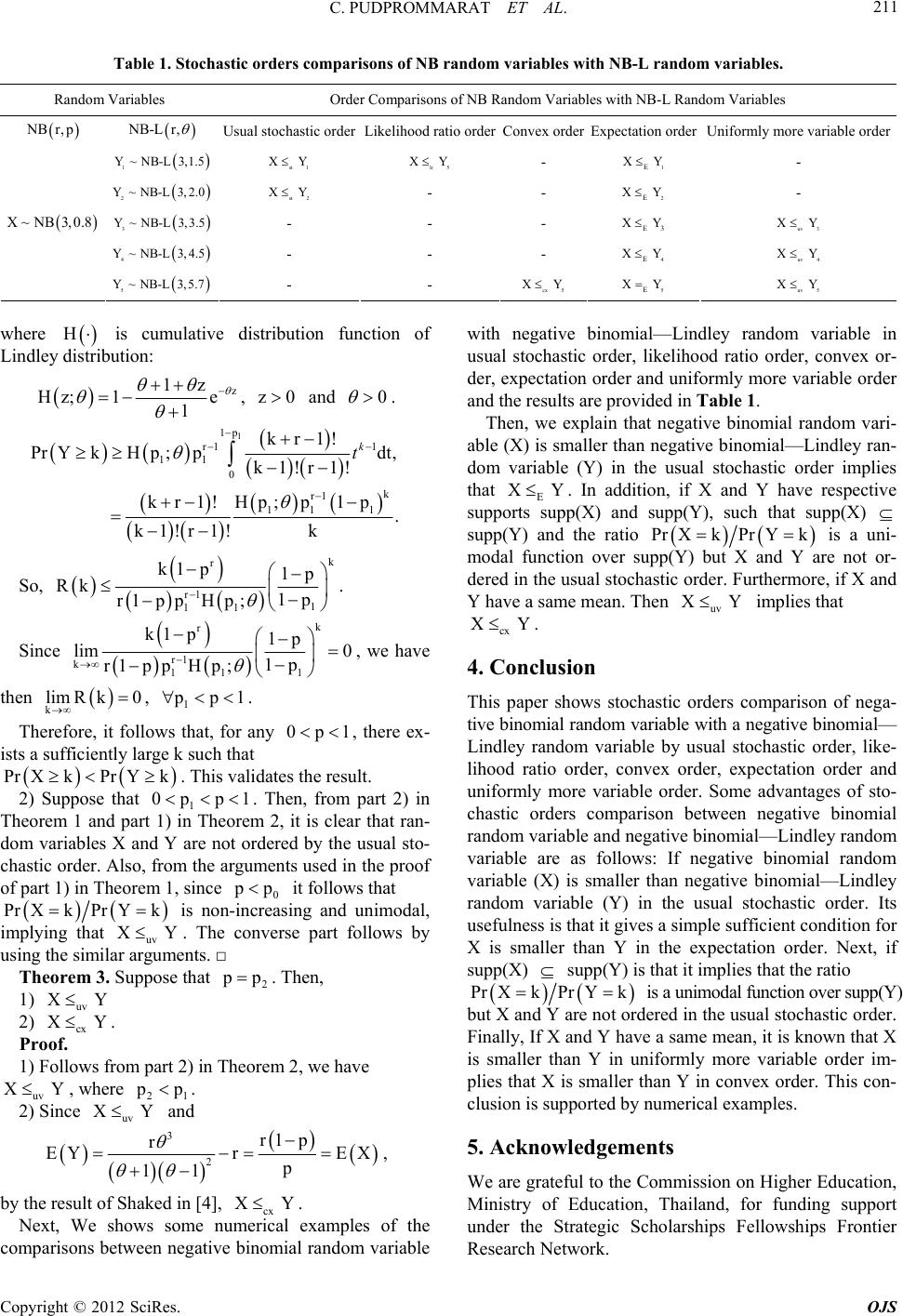. PUDPROMMARAT ET AL.
211
Table 1. Stochastic orders comparisons of NB random variables with NB-L random variables.
Random Variables Order Comparisons of NB Random Variables with NB-L Random Variables

NBr, p

NB-Lr,

Usual stochastic orderLikelihood ratio orderConvex orderExpectation order Uniformly more variable order

B-L 3,1.5
1
Y~N st lr 5 XY 1E XY -
2
Y~N st 2 XY 2E XY -

3
Y~NB-L3,3.5 - - -
E3
XYuv 3 XY

4
Y~NB-L3,4.5 - - -
E
XYuv 4 XY

5
Y~NB-L3,5.7 E XYuv 5 XY
1
XY -

B-L3,2.0 - -
4

X~NB 3,0.8
- -
cx 5
XY5
where

H is cumulative distribution function of
Lindley distribution:

z
1z
e
1
Hz; 1





, z0 and 0
 

.





 
1
1p
r1 1
k
r1
11
kr1!
Pr YkHdt,
1!Hp; p
1
k
t





 


11
0k1
!r1!
p ;p
r
k1!r



1
1p. k
 ! k
So,
  
k
r1
11
p1p
Rk 1p
r1 pp Hp;







.


r
1
k1
Since
 
k r
11
k1 p1p
lim 0
1p r1 ppH; 





 
, we have
then

r1
k1
p

k
lim Rk0, 1
p
p1.
lidates the result.
ose that The part 2) in
2, it is clear that ran-
domd Y are not ordered by the usual sto-
chastfrom the arguments used in the proof
of pa 1, since 0
Thert follows that, for any 0p1, there ex-
ists a sufficiently large k such that

PrXk PrYk
efore, i

. This va
1
0p p
rt 1) in Theorem
2) Supp
Theorem
1.n, from
1 and pa
variables X an
ic order. Also,
rt 1) in Theorem
p
p it follows that

Pr s non-increasing and unimodal,
hat . The converse part follows by
mints. □
hat 2
XkPrYk i
uv
XY
lar argume
Suppose t
implying t
using the si
Theorem 3.
p
p

. Then,
uv

2) cx XY
ows from part 2) in Theorem 2, we ha
, where 1
1) XY
.
Proof.
1) Follve
uv
XY2
p
p.
uv
XY and 2) Since
 

3
2
r1
r
EYr X
p
11


 
 ,
pE 
byed in [4], X
with negative binomial—Lindley random variable in
usual stochastic order, likelihood ratio order, convex or-
der, expectation order and uniformly more variable order
and the results are provided in Table 1.
Then, we explain that negative binomial random vari-
able (X) is smaller than negative binomial—Lindley ran-
order implies
that XY
dom variable (Y) in the usual stochastic

E. In addition, if X and Y have respective
supp(X)  supports supp(X) and supp(Y), such that
supp(Y) and the ratio


PrX kPrYk is a uni-
modal funtion over supp but X and Ye not or-
dered in t usual stochast order. Furthermre, if X and
Y have a same mean. Thenuv XY implthat
cx
XY
c
he
(Y)
ic
ar
o
ies

.
4. Conclusion
This paper shws stochast orders comparisof nega-
tive binomial random variable with a negative binomial—
, exd
uniformly more variab
compari
inomial—Lindley random
vanegatiial random
vale (X) is smaller than negative binomial—Lindley
ram variab (Y) in the usual stochastic order. Its
us is that it gives a simple sufficient condition for
Xxt, if
supp(X) (Y) is tt it implies that the ratio
oicn o
Lindley random variable by usual stochastic order, like-
lihood ratio order, convex orderpectation order an
le order. Some advantages of sto-
chastic orders son between negative binomial
random variable and negative b
riable are as follows: If ve binom
riab
ndo le
efulness
is smaller than Y in the expectation order. Ne
 suppha




the result of Shakcx Y.
Next, We shows some numerical examples of the
comparisons between negative binomial random variable
PrPr YkXk

nimodal function over supp(Y)
but X and Y are not ordered in the usual stochasticr.
Finally, If X and Y have a same mean, it is known X
is smaller than Y in uniformly more variable order im-
n converder. This con-
cl
R
is a u
orde
that
plies that X is smaller than Y ix o
usion is supported by numerical examples.
5. Acknowledgements
We are grateful to the Commission on Higher Education,
Ministry of Education, Thailand, for funding support
under the Strategic Scholarships Fellowships Frontier
esearch Network.

C. PUDPROMMARAT ET AL.
212
REFERENCES
[1] W. Rainer, “Econometric Analysis of Count Data,” 3rd
Edition, Springer-Verlag, Berlin, 2000.
[2] H. Zamani and N. Ismaal—Lindley
Distribution and Its Application,” Journal of Mathematics
and Statistics, Vol. 6, No. 1, 2010, pp. 4-9.
il, “Negative Binomi
doi:10.3844/jmssp.2010.4.9
[3] M. Shaked and J. G. Shanr, “Stochastic Ordthikuma
Academic Press, New York, 2006.
Stochastic Processes,” Wiley, New York,
ers,”
[4] S. M. Ross, “
1983.
[5] N. Misra, H. Singh and E. J. Harner, “Stochastic Com-
parisons of Poisson and Binomial Random Variables with
Their Mixtures,” Statistics and Probability Letters, Vol.
65, No. 4, 2003, pp. 279-290.
doi:10.1016/j.spl.2003.07.002
[6] M. Shaked, “On Mixtures from Exponential Families,”
Journal of the Roy
No. 2, 1980, pp. 192-198.
al Statistical Society: Series B, Vol. 42,
[7] M. Shaked an“Stochastic Orders
and Their ApPress, New York,
fe Distributions,”
d J. G. Shanthikumar,
plications,” Academic
1994.
[8] H. Singh, “On Partial Orderings of Li
Naval Research Logistics, Vol. 36, No. 1, 1989, pp. 103-
110.
doi:10.1002/1520-6750(198902)36:1<103::AID-NAV322
0360108>3.0.CO;2-7