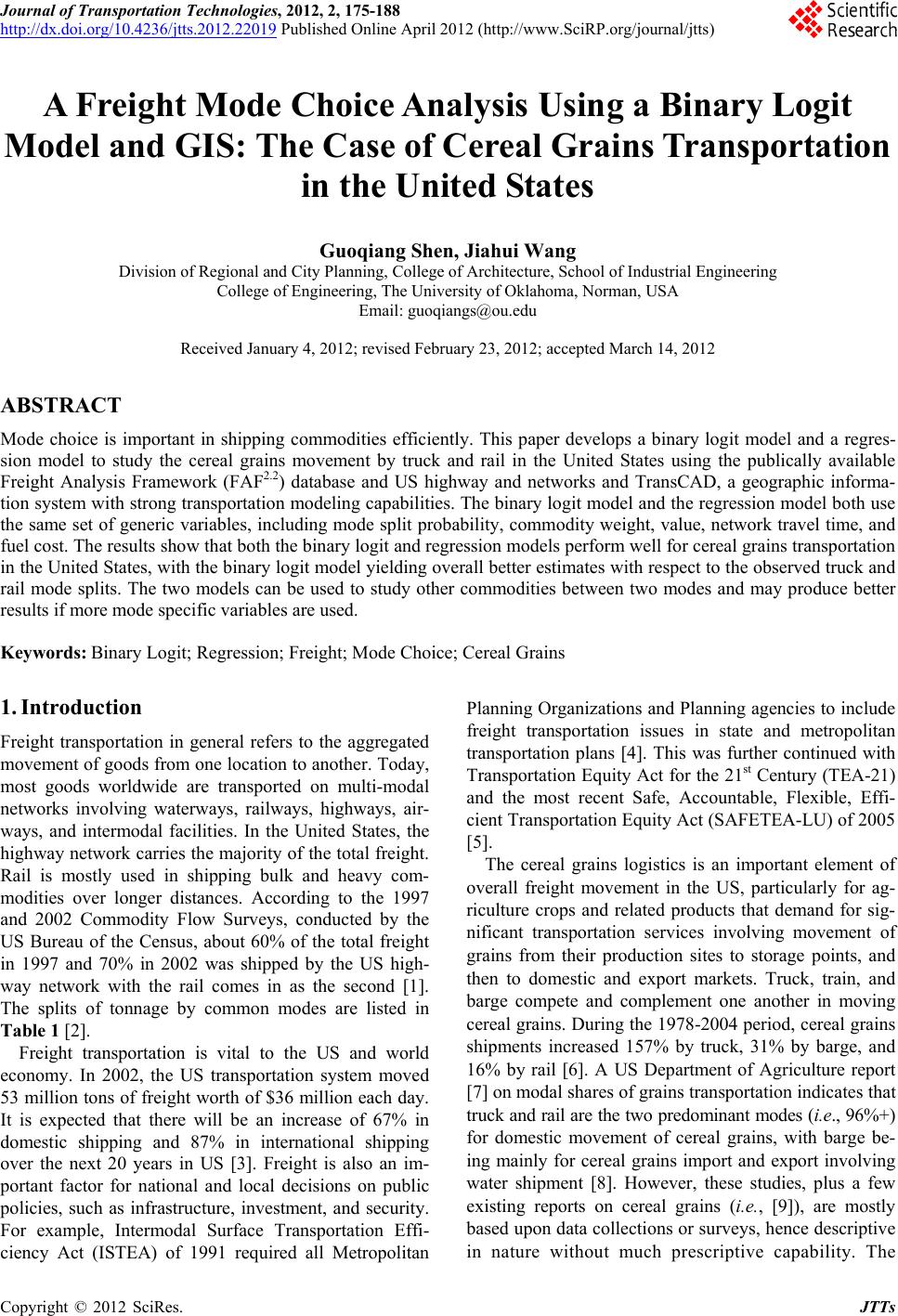Journal of Transportation Technologies, 2012, 2, 175-188
http://dx.doi.org/10.4236/jtts.2012.22019 Published Online April 2012 (http://www.SciRP.org/journal/jtts)
A Freight Mode Choice Analysis Using a Binary Logit
Model and GIS: The Case of Cereal Grains Transportation
in the United States
Guoqiang Shen, Jiahui Wang
Division of Regional and City Planning, College of Architecture, School of Industrial Engineering
College of Engineering, The University of Oklahoma, Norman, USA
Received January 4, 2012; revised February 23, 2012; accepted March 14, 2012
ABSTRACT
Mode choice is important in shipping commodities efficiently. This paper develops a binary logit model and a regres-
sion model to study the cereal grains movement by truck and rail in the United States using the publically available
Freight Analysis Framework (FAF2.2) database and US highway and networks and TransCAD, a geographic informa-
tion system with strong transportatio n modeling capabilities. The binary logit model an d the regression model both use
the same set of generic variables, including mode split probability, commodity weight, value, network travel time, and
fuel cost. The results show th at both th e binary lo git and regression models perform well for cer eal grains transp ortation
in the United States, with the binary logit mod el yielding overall better estimates with respect to the observed truck an d
rail mode splits. The two models can be used to study other commodities between two modes and may produce better
results if more mode specific variables are used.
Keywords: Binary Logit; Regression; Freight; Mode Choice; Cereal Grains
1. Introduction
Freight transportation in general refers to the aggregated
movement of goods from one location to another. Today,
most goods worldwide are transported on multi-modal
networks involving waterways, railways, highways, air-
ways, and intermodal facilities. In the United States, the
highway network carries the majo rity of the total freight.
Rail is mostly used in shipping bulk and heavy com-
modities over longer distances. According to the 1997
and 2002 Commodity Flow Surveys, conducted by the
US Bureau of the Census, about 60% of the total freight
in 1997 and 70% in 2002 was shipped by the US high-
way network with the rail comes in as the second [1].
The splits of tonnage by common modes are listed in
Table 1 [2].
Freight transportation is vital to the US and world
economy. In 2002, the US transportation system moved
53 million tons of freight worth of $36 million each day.
It is expected that there will be an increase of 67% in
domestic shipping and 87% in international shipping
over the next 20 years in US [3]. Freight is also an im-
portant factor for national and local decisions on public
policies, such as infrastructure, investment, and security.
For example, Intermodal Surface Transportation Effi-
ciency Act (ISTEA) of 1991 required all Metropolitan
Planning Organizations and Planning agencies to include
freight transportation issues in state and metropolitan
transportation plans [4]. This was further continued with
Transportation Equity Act for the 21st Century (TEA-21)
and the most recent Safe, Accountable, Flexible, Effi-
cient Transportation Equity Act (SAFETEA-LU) of 200 5
[5].
The cereal grains logistics is an important element of
overall freight movement in the US, particularly for ag-
riculture crops and related products that demand for sig-
nificant transportation services involving movement of
grains from their production sites to storage points, and
then to domestic and export markets. Truck, train, and
barge compete and complement one another in moving
cereal grains. During the 1978-2004 period, cereal grains
shipments increased 157% by truck, 31% by barge, and
16% by rail [6]. A US Department of Agriculture report
[7] on modal shares of grains transportation indicates that
truck and rail are the two predominant modes (i.e., 96%+)
for domestic movement of cereal grains, with barge be-
ing mainly for cereal grains import and export involving
water shipment [8]. However, these studies, plus a few
existing reports on cereal grains (i.e., [9]), are mostly
based upon data collections or surveys, hence descriptive
in nature without much prescriptive capability. The
C
opyright © 2012 SciRes. JTTs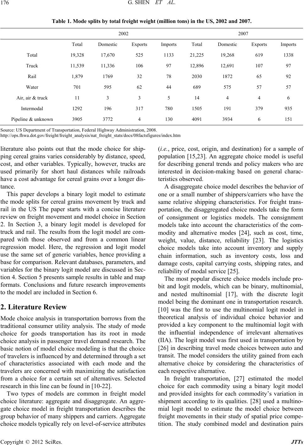

G. SHEN ET AL. 176
Table 1. Mode splits by total freight weight (million tons) in the US, 2002 and 2007.
2002 2007
Total Domestic Exports Imports Total Domestic Exports Imports
Total 19,328 17,670 525 1133 21,225 19,268 619 1338
Truck 11,539 11,336 106 97 12,896 12,691 107 97
Rail 1,879 1769 32 78 2030 1872 65 92
Water 701 595 62 44 689 575 57 57
Air, air & truck 11 3 3 5 14 4 4 6
Intermodal 1292 196 317 780 1505 191 379 935
Pipeline & unknown 3905 3772 4 130 4091 3934 6 151
Source: US Department o f Transportation, Federal Highway Administration, 2008.
http://ops.fhwa.dot.gov/freight/freight_analysis/nat_freight_stats/docs/08factsfigures/index.htm
literature also points out that the mode choice for ship-
ping cereal grains varies considerably by distance, speed,
cost, and other variables. Typically, however, trucks are
used primarily for short haul distances while railroads
have a cost advantage for cereal grains over a longer dis-
tance.
This paper develops a binary logit model to estimate
the mode splits for cereal grains movement by truck and
rail in the US The paper starts with a concise literature
review on freight movement and model choice in Section
2. In Section 3, a binary logit model is developed for
truck and rail. The results from the logit model are com-
pared with those observed and from a common linear
regression model. Here, the regression and logit model
use the same set of generic variables, hence providing a
base for comparison. Relevant databases, parameters, and
variables for the binary logit model are discussed in Sec-
tion 4. Section 5 presents sample results in table and map
formats. Conclusions and future research improvements
to the model are included in Sectio n 6.
2. Literature Review
Mode choice analysis in transportation borrows from the
traditional consumer utility analysis. The study of mode
choice for goods transportation has its root in mode
choice analysis in passenger travel demand research. The
basic notion of model choice modeling is that the choice
of travelers is influenced by and determined through a set
of characteristics associated with each mode and the
travelers are concerned with maximizing the satisfaction
from a choice for a certain set of alternatives. Selected
research in this line can be found in [10-22].
Two types of models are common in freight model
choice literature: aggregate and disaggregate. An aggre-
gate choice model in freight transportation describes the
group behavior of many shippers and carriers. Aggregate
choice models typically rely on level-o f-service attributes
(i.e., price, cost, origin, and destination) for a sample of
population [15,23]. An aggregate choice model is useful
for describing general trends and policy makers who are
interested in decision-making based on general charac-
teristics observed.
A disaggregate choice model describes the behavior of
one or a small number of shippers/carriers who have the
same relative shipping characteristics. For freight trans-
portation, the disaggregated choice models take the form
of consignment or logistics models. The consignment
models take into account the characteristics of the com-
modity and alternative modes [24], such as cost, time,
weight, value, distance, reliability [23]. The logistics
choice models take into account inventory and supply
chain information, such as inventory costs, loss and
damage costs, capital carrying costs, shipping rates, and
reliability of modal service [25].
The most popular discrete choice models include pro-
bit and logit models, which can be binary, multinomial,
and nested multinomial [17], with the discrete logit
model being the dominant one in transportation research.
[10] was the first to use the multinomial logit model in
theoretical analysis of individual choice behavior and
provided a key component to the multinomial logit with
the influential independence of irrelevant alternatives
(IIA). The logit model was first used in transportatio n by
[26] in describing travel mode choices between auto and
transit. The model considers the utility gained from each
alternative choice by considering the characteristics of
each respective alternative.
In freight transportation, [27] estimated the model
choice for each commodity using a binary logit model
and provided insights for each commodity’s variation in
shipment according to its qualities. [28] used a multino-
mial logit model to estimate the model choice between
freight movements in their study of spatial price compe-
tition. The study combined model and destination pairs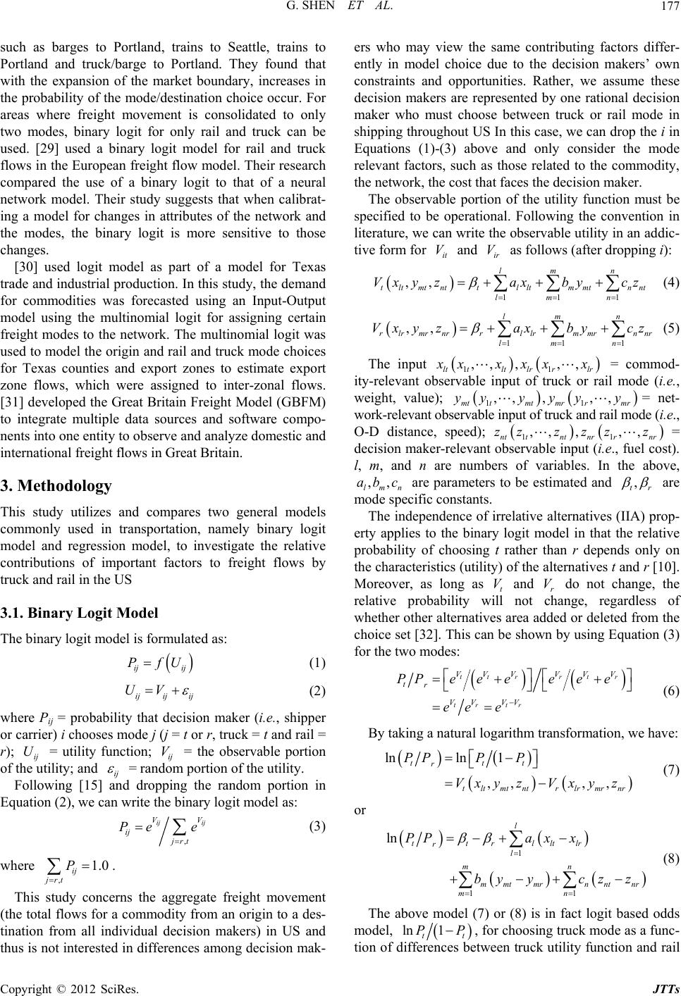

G. SHEN ET AL. 177
such as barges to Portland, trains to Seattle, trains to
Portland and truck/barge to Portland. They found that
with the expansion of the market boundary, increases in
the probability of the mode/destination choice occur. For
areas where freight movement is consolidated to only
two modes, binary logit for only rail and truck can be
used. [29] used a binary logit model for rail and truck
flows in the European freight flow model. Their research
compared the use of a binary logit to that of a neural
network model. Their study suggests that when calibrat-
ing a model for changes in attributes of the network and
the modes, the binary logit is more sensitive to those
changes.
[30] used logit model as part of a model for Texas
trade and industrial production. In this study, the demand
for commodities was forecasted using an Input-Output
model using the multinomial logit for assigning certain
freight modes to the network. The multinomial logit was
used to model the origin and rail and truck mode choices
for Texas counties and export zones to estimate export
zone flows, which were assigned to inter-zonal flows.
[31] developed the Great Britain Freight Model (GBFM)
to integrate multiple data sources and software compo-
nents into one entity to observe and analyze d omestic and
international freight flows in Great Britain.
3. Methodology
This study utilizes and compares two general models
commonly used in transportation, namely binary logit
model and regression model, to investigate the relative
contributions of important factors to freight flows by
truck and rail in the US
3.1. Binary Logit Model
The binary logit model is formulated as:

ij ij
P
fU (1)
ijij ij
UV

 (2)
where Pij = probability that decision maker (i.e., shipper
or carrier) i chooses mode j (j = t or r, truck = t and rail =
r); ij = utility function; ij = the observable portion
of the utility; and
U V
ij

= rando m portion of the utility.
Following [15] and dropping the random portion in
Equation (2), we can write the binary logit model as:
,
ij ij
V
ij jrt
Pe e

V

(3)
where .
,1.0
ij
jrt
P



This study concerns the aggregate freight movement
(the total flows for a commodity from an origin to a des-
tination from all individual decision makers) in US and
thus is not interested in differences among decision mak-
ers who may view the same contributing factors differ-
ently in model choice due to the decision makers’ own
constraints and opportunities. Rather, we assume these
decision makers are represented by one rational decision
maker who must choose between truck or rail mode in
shipping throughout US In this case, we can drop the i in
Equations (1)-(3) above and only consider the mode
relevant factors, such as those related to the commodity,
the network, the cost that faces the decision maker.
The observable portion of the utility function must be
specified to be operational. Following the convention in
literature, we can write the observable utility in an ad dic-
tive form for and as follow s (a ft er dr o pping i):
it
Vir V

11 1
,, lm n
tltmtnt tlltmmtnnt
lm n
Vxy zaxbycz 
 
 
 
(4)

11 1
,, lm n
rlrmrnr rllrmmrnnr
lm n
Vxy zaxbycz 
 
 
 
(5)
The input


11
,, ,,,
lt tltlr rlr

x
xxxxx = commod-
ity-relevant observable input of truck or rail mode (i.e.,
weight, value);


1
,, ,,
mt tmtmr r

1mr
,
y
yyyyy= net-
work-relevant observable input of truck and rai l mode (i.e.,
O-D distance, speed);


,, ,
nt tntnr
z z

11r nr
zz =
decision maker-relevant observable input (i.e., fuel co st).
l, m, and n are numbers of variables. In the above,
are parameters to be estimated and
,z
,
t
,z
r
,,
lmn
ab c

 are
mode specific constants.
The independence of irrelative alternatives (IIA) prop-
erty applies to the binary logit model in that the relative
probability of choosing t rather than r depends only on
the characteristics (utility) of the alternatives t and r [10].
Moreover, as long as and do not change, the
relative probability will not change, regardless of
whether other alternatives area added or deleted from the
choice set [32]. This can be shown by using Equation (3)
for the two modes:
t
Vr V


tt t rr r
ttr r
VV V VV V
tr
VVV V
PPe eeeee
ee e


 
 

 
 (6)
By taking a natural logarithm transformation, we have:





lnln 1
,, ,,
ttt
r
tltmtnt rlrmrnr
PPP P
Vxy zVxyz
 



(7)
or



1
11
ln l
ttrl ltlr rl
mn
mmtmrn ntnr
mn
PPa xx
byyczz



 




(8)
The above model (7) or (8) is in fact logit based odds
model,


ln 1
tt
, for choosing truck mode as a func-
tion of differences between truck utility functio n and rail
PP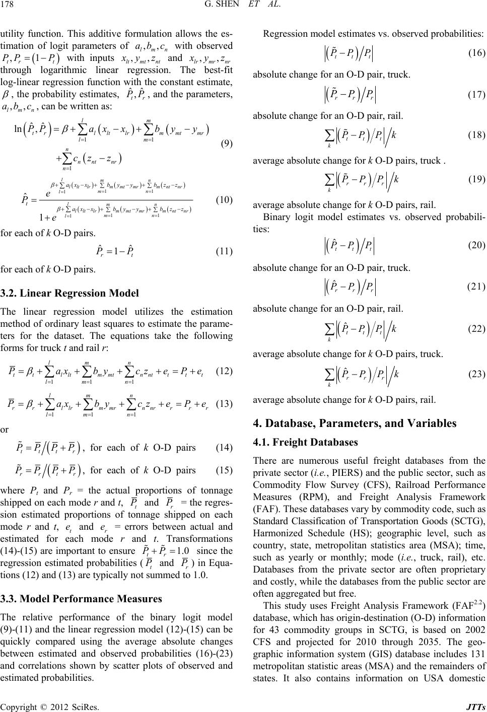

G. SHEN ET AL. 178
utility function. This additive formulation allows the es-
timation of logit parameters of with observed
with inputs ltmt nt
,,
lmn
ab c
,,

,1
tr t
PP P

x
yz and ,,
lrmr nr
x
yz
through logarithmic linear regression. The best-fit
log-linear regression function with the constant estimate,

, the probability estimates, , and the parameters,
, can be written as:
ˆ

1
lr
nr
x


ˆ
,
tr
PP

lm
m
lm
b



,,
lmn
ab c

ˆˆ
ln ,
t r
n
PP

1
l ltmt
n
nnt
a xy
czz







1
mr
y


(9)

 
11
11
mn
mr mnt
mn
mtmrm
mn
ybz
y b


 


ˆ
t
P
1
ˆ
1
l
l
te
P
e





1
ll t lrmnr
ln
lltlrnt
l
ax xbz
ax xbz




mt
m
m
y
y

nr
z
(10)
for each of k O-D pairs.
ˆ
1
r
P (11)
for each of k O-D pairs.
3.2. Linear Regression Model
The linear regression model utilizes the estimation
method of ordinary least squares to estimate the parame-
ters for the dataset. The equations take the following
forms for truck t and rail r:
11
lm
t llt m
lm
Paxb

 
 1
n
nntt
n
cz



t
  mt ytt ePe (12)
11
lm
r rllrm
lm
Pax 


 1
n
nnrr
n
cz



mr
byrr ePe (13)
or

tttr
PPPP
, for each of k O-D pairs (14)

rrtr
P
PPP
, for each of k O-D pairs (15)
where Pt and Pr = the actual proportions of tonnage
shipped on each mode r and t, t P and r P
tr
PP

= the regres-
sion estimated proportions of tonnage shipped on each
mode r and t, and = errors between actual and
estimated for each mode r and t. Transformations
(14)-(15) are important to ensure since the
regression estimated probabilities (
t
er e
1.0
t
P and r P) in Equa-
tions (12) and (1 3) are typically not summed to 1.0.
3.3. Model Performance Measures
The relative performance of the binary logit model
(9)-(11) an d the linear regression model (12)-(15 ) can be
quickly compared using the average absolute changes
between estimated and observed probabilities (16)-(23)
and correlations shown by scatter plots of observed and
Regression model esti
mated probabilities.
mates vs. observed probabilities:
esti


ttt
PPP
 (16)
absolute change fo r an O-D pair, truck.


rrr
P
PP
 (17)
absolute change fo r an O-D pair, rail.


ttt
k
PPPk
 (18)
average absolute change for k O-D pairs, truck .


rrr
k
PPPk
 (19)
average absolute change for k O-D pairs, rail. probabili-
tieBinary logit model estimates vs. observed s:


ˆttt
PPP (20)
absolute change fo r an O-D pair, truck.


ˆ
PPP
rrr (21)
absolute change for an O-D pair, rail .


ˆ
PPPk

ttt
k
(22)
average absolute change for k O-D pairs, truck.


ˆ
PPPk

rrr
k
(23)
average absolute change for k O-D pairs, rail.
4. Database, Parameters, and Variables
freight databases from the
Analysis Framework (FAF)
da
states. It also contains information on USA domestic
4.1. Freight Databases
There are numerous useful
private sector (i.e., PIERS) and the pub lic sector, such as
Commodity Flow Survey (CFS), Railroad Performance
Measures (RPM), and Freight Analysis Framework
(FAF). These databases vary by commodity code, such as
Standard Classification of Transportation Goods (SCTG),
Harmonized Schedule (HS); geographic level, such as
country, state, metropolitan statistics area (MSA); time,
such as yearly or monthly; mode (i.e., truck, rail), etc.
Databases from the private sector are often proprietary
and costly, while the databases fro m the public sector are
often aggregat ed but free.
This study uses Freight 2.2
tabase, which has origin-d estination (O-D) in formation
for 43 commodity groups in SCTG, is based on 2002
CFS and projected for 2010 through 2035. The geo-
graphic information system (GIS) database includes 131
metropolitan statistic areas (MSA) and the remainders of

G. SHEN ET AL. 179
shipments in value and weight by mode. The latest
available FAF3.0 is based on 2007 CFS and projected for
2010 to 2040. However, FAF2.2 contains virtually the
same information on mode, value, weight, commodity,
and O-D pairs as FAF2.2 does.
There are also some highway and rail network data-
bases in a GIS format, such as North American Trans-
po
US Ac-
co
one shipment of cereal grain using
tru
ameters and Variables
aracteristics of the
ode. In general it is
and railroad. For each mode, the
ge
odity Variables
The generic characteristics of the commodity shipment
onnage and dollar value.
rtation Atlas Data (NTAD) from the Bureau of Trans-
portation Statistics (BTS), the intermodal highway
transportation netwo rk by Oak Ridge Nation al Laborato-
ries (ORNL), FAF2.2 highway network in Shape GIS
format. This study utilizes the 2006 NTAD truck and rail
networks proce ssed wi t hi n TransC A D 4. 8 [3 3].
The study area and data used for this research are all
cereal grains shipments by rail and truck in the
rding to BTS, cereal grains freight comprised of ap-
proximately 7% of all freigh t moved in the US dur ing the
year 2002 [34]. The FAF2.2 dataset describes the cereal
grains commodity according to the SCTG coding scheme.
This commodity class includes multiple types of grain
including but not exclusive to unsweetened corn, wheat,
rye, barley, and oats .
The dataset contains 11 origins and 22 destinations
each receiving at least
ck and rail. For validation of the model choice analy-
sis, only origins and destinations (O-D) which sent and
received cereal rain by truck and rail were considered.
Other O-Ds which shipped only by truck or only by rail
were excluded because of the possibility that a modal
choice could not take place. Intermodal choices that may
occur somewhere on the route to a destination were not
considered in this study. Some outliers (about 10) were
also excluded. As a consequence the dataset used as in-
put to the binary logistic model contains about 60 obser-
vations.
4.2. Par
The parameters consist of both ch
shipment and characteristics of the m
helpful to use alternative specific variables. Alternative
specific variables are those which vary across modes.
However, since the mode specific information is often
unavailable, variables which provide generic measure-
ment for all modes are useful. Generic characteristics are
those attributes that are indistinguishable between modes.
The generic features of the shipment, such as tonnage
and value, apply to all modes, though the actual magni-
tudes of tonnage and value for each shipment may be
different [35]. So are the network features, such as travel
distance or speed or time, and energy use features, such
as fuel consumption.
For this study, variables were chosen to describe two
different modes: truck
neric variables are used to construct the utility function
for a mode. The parameters and variables are listed in
Table 2.
4.2.1. Comm
take the form of shipment t
These measurements for the commodity are given in
units of tons and millions of US dollars. The variables
are denoted 11
,
tr
x
x in Table 2.
4.2.2. Netw oriables rk Va
The rail and truck transportation networks are totally
e set of origins and destina-
Estimating the cost of freight transportation is a chal-
uch difficulty in determining
odel.
different. However, the sam
tions for cereal grains are used for both networks. Ori-
gins and destinations were connected to each network.
The attribute file for the railroad and highway network
provides the length of each link in the network. Tran-
sCAD’s multiple shortest path function was used to
compute the shortest path distance for each origin and
destination. O-D shortest path distances were recorded
for both networks. The speed values include the stop
times for trucks and the dwell times for rail shipments.
The speed values for railroads were taken from the Rail-
road Performance Measures dataset [36]. Their dataset is
a compilation of US railroad information including av-
erage speeds and average dwell times for railroad desti-
nations. The truck speeds were taken from a study con-
ducted by the American Transportation Research Insti-
tute [37]. The travel time is calculated by distance for
each O-D divided by the speed of the mode for the O-D
pair. The variables are denoted 11
,
tr
yy in Table 2.
4.2.3. Fuel Cost Variable
lenging task and there is m
all the costs which contribute to the overall cost of
freight movement precisely. The following formula (24)
Table 2. Parameters and variables used in the binary logit
m
ParameterVariable Description Type

Regression Constantconstant
1
a 11 ,
tr
x
x Weight in tons of
a shipment Generic
2
a 22 ,
tr
x
x Value in dollars of
a shipment Generic
1
b 11 ,
tr
yy Shortest network
distance for an O-D pair
ce/
ent
Generic
2
b 22 ,
tr
yy Travel time = distan
speed Generic
1
c 11 ,
tr
zz Fuel cost per ton-mile of
a shipmGeneric

G. SHEN ET AL. 180
was used for estimating ers
shipme gallons of fuel per ton-mile. Similarly, Truck Fuel Cost
per ton-mile = 5,104,160 billion/1,360,760 million =
3750.96 BTU’s per ton-mile. 3750.96/138,700 = 0.027
gallons of fuel per ton-mile. Here, 138,700 = Amount of
British Thermal Units equal to one gallon of diesel fuel.
the cost of fuel for ceal grain
nts.

jj
F
rb

 (24)
where j = mode;
j
r
red as th
di
= British th
ton-mile (measue total BTU con
ermal units (BTU) per
sumed for that A sample of the data input to the binary logit model is
listed in Table 4. Here the origins and destinations are
based on state MSAs and state reminders (rem). Com-
modity type is cereal grains, including Wheat, Barley,
Oats, Corn, etc. The unit for shipment value is million
dollars, for time hours, for fuel dollar per ton-mile, and
for distance mile.
year for the mode vided by the total ton-miles for the
mode)1; b = Number of BTU’s equal to one gallon of fuel
(138,700)2;

= Fuel cost ($/gallon) per gallon2;
j
F
=
Fuel cost per ton-mile mode j.
This measrement was originally used for the puose
of comparing the use of fuel
u rp
in freight transportation
am
2002 data in Table 3. Rail Fuel Cost per
to
ong modes and their relative energy efficiency [38].
This is done by taking the total amount of fuel consumed
in BTU’s for the mode in the year 2002 and dividing this
by the total amount of ton-miles for the mode in the year
2002. The cost of fuel per gallon was averaged for the
year 2002 for both railroad and highway [2]. These cal-
culations provided an estimate for the fuel co st in gallons
per ton-mile for each mode. The variables are denoted in
Table 2.
Calculations for truck and railroad fuel cost are based
on the following
5. Results and Analysis
The binary logit model was tested in TransCAD 4.8. [33].
Table 3. US truck and rail ton-miles, btus, and fuel con-
sumption in 2002.
Mode Ton-Miles in 2002 in
millions
BTU consumed
in 2002 in
trillions
Gallons of fuel
used in 2002 in
millions
Rail 1,261,813 520 3751.413
Truck1,360,760 5104 36,800
n-mile = 520320.9831 billion/1,261,813 million =
412.36 BTU’s per ton-mile. 412.36/138,700 = 0.00297 Source: [39] and [2]
Table 4. A sample data input to the binary logit model.
Origin Destination Commodity Mode Tons Dollar Time Fuel Cost/TM Distance
IL rem IN rem Cereal grains Truck 220,94014.44.540.02700 2 23.0
IL rem OH rem Cereal grains
1
1 1
a 1,417
a a 3,618
12.9
em rem eal grains 35,73.24.0.00249
2,4 6
1 2.
3 36
1 1
a
a a
… …
Truck 28000.149.460.02700 4 64.3
IN rem IL rem Cereal grains Truck 354,0908.134.540.02700 223.0
IN rem IL St Lo Cereal grains Truck 76200.384.810.02700 236.0
IN rem KY rem Cereal grains Truck 465,66023.493.120.02700 153.3
IN rem PA rem Cereal grains Truck 4,9101.641.840 .02700 581.4
IN rem VA rem Cereal grains Truck 18, 2201.099.200.02700 451.9
KS KansKS rem Cereal grains Truck 96,6109.544.180.02700 205.4
KS KansMO KansCereal grains Truck 00,3905.071.040.02700 51.1
KS Kansa TX DallaCereal grains Truck 31,82011.859.610.02700 471.8
… … … … ………… …
IL rem IN rem Cereal grains Rail 21,1701.6345850.00297 265. 4
IL rOH CerRail40840697 3.2
IN rem IL rem Cereal grains Rail 70,5304.0412.945850.00297 265.4
IN rem IL St Lo Cereal grains Rail 28,9103.55675610.00297 54.9
IN rem KY rem Cereal grains Rail 91,45031.577.1497560.00297 146.6
IN rem PA rem Cereal grains Rail 310,5003.092.169 760.00297 59.5
IN rem VA rem Cereal grains Rail 94,41008.1425.888780.00297 530.7
KS KansKS rem Cereal grains Rail 44,86011.249.5960980 .00297 196.7
KS KansMO KansCereal grains Rail 266,87021.093.3682930 .00297 69.1
… …… …… … …
1The computation for British thermal units per ton-mile was confirmed by Eastman (1981).
2These measurements were given in t he Transportation Ener gy Data Book [39].

G. SHEN ET AL. 181
Tle screen shots are gure nd 2.
Thbserved m split probaties and prob-
l
e m
tir
e spuch to10% ruck or
ersa, thlogit angression eates are relatively
wo sampshown in Fis 1 a
e oodebilithe
abilities estimated from the binary logit model for rai
an Tables 56d truck are listed in and . It is interesting to
see that some observed (,
tr
PP = observed probabilities)
and estimated probabilities (ˆˆ
,
tr
PP
= probabilities from
the logit model, ,
tr
PP

= probabilities from the regres-
sion model) are very close for some O-D pairs for the
truck mode, such as OD28, OD27, and OD20 (t P = 0.52,
ˆt
P = 0.56, t P
 = 0.52), but are quite off for OD21, OD12,
and OD1(t
P = 0.09, ˆt P = 0.47, t P
 = 0.47), while most
oher O-D pairs, such as OD30, OD16, and OD2 (t
P =
0.93, ˆt P = 0.73, t P
 = 0.58) are neither too much close
or off. Similar results can be found for the rail mode.
Interstingly, soe O-D pairs with relatively good
logit and regression results for one mode are not neces-
sar
t
ily good for the other mode, such as OD22 for truck
(t
P = 0.98, ˆt
P = 0.71, t P
 = 0.55) and OD22 for rail
(r
P = 0.02, ˆr P = 0.29, r P
 = 0.45), while certain O-D
airs are relative goo opd forth models, such as OD23. It
h s
b
seems that fore O-D pa with extremely unbalanced
modlits, s as 90%ail to tr vice
veir d restim
worse than those nodes with more balanced modal splits,
such as 40% to 60% rail to truck or vice versa. Indeed,
Tables 5 and 6 both have the last two columns showing
the absolute changes between the estimated vs. the ob-
served probabilities. Those O-D pairs with large changes
(i.e., larger than 2.0) have their estimates off 3 times
more or less than their observed probabilities with some
O-D pairs fair better with rail and others with truck.
However, the overall averages (1.38 vs. 2.14 for rail and
0.74 vs. 1.75 for truck) indicate that the logit model per-
forms better.
Figures 3-8 illustrate the observed and estimated tru ck
and rail flows assigned to the national truck and rail net-
works in 2002. In these figures, the truck or rail
links/paths with assigned cereal grains flows are high-
lighted and scaled in back color. The highway and rail
segments without carrying cereal grains flows are shown
in gray color. These figures are referenced with state
boundaries.
Figure 1. A sample of input data screen.

G. SHEN ET AL. 182
Figure 2. A sample of output probability screen.
As visually shown in these figures, the cereal grains
movement spread out within the US, but more concen-
trated in the middle of US or America’s plain region cen-
tered around Kansas from which cereal grains were
moved to north-south and east-we st in the US Comparing
these figures and checking the observed and estimated
mode splits in Tables 5 and 6 also show that overall both
binary logit model and linear regression estimates work
well with just the usage of few generic variables. How-
ever, the binary logit model performs better, as shown in
Figures 9 and 10, that binary logit model estimates
(green color) are more in line with the values and varia-
tions of actual percentages or probabilities (black color)
than the regression estimates (brown color) for the two
modes for cereal grains movement in the US Regression
estimates are generally less fluctuated among the origin
and destinations pairs
Scatter plots of Figures 11 and 12 of actual mode
splits vs. logit or regression estimates further indicate
that the logit model (green color), with higher R-square
or correlation values, generally outperforms the regres-
sion model (brown color).
6. Conclusions and Remarks
This paper concisely reviewed relevant literature on
mode splits for freight movement, developed a binary
logit model for truck and rail, tested the model for cereal
grains movement in the United States in 2002 using
TransCAD, and compared the model results with those
from a comparable linear regression model. The overall
probability estimates from the binary logit mod el and the
regression model, as compared with the observed mode
splits of truck and rail, are better for some O-D pairs than
others. However, the logit model outperforms the linear
regression model in general in terms of smaller average
absolute percentage changes and better correlations be-
tween estimated and ob served mode probabilities.
The binary logit model also can be applied to other
commodities as long as they are transported predomi-
nantly by two modes, such as rail and water or truck and
water. The input data are at the lev els of state MSAs and
reminders, but better results, particularly for flow as-
signments, can be achieved if finer geographic units,
such as traffic analysis zones, are used. A specific index
may be designed to measure the aggregated deviations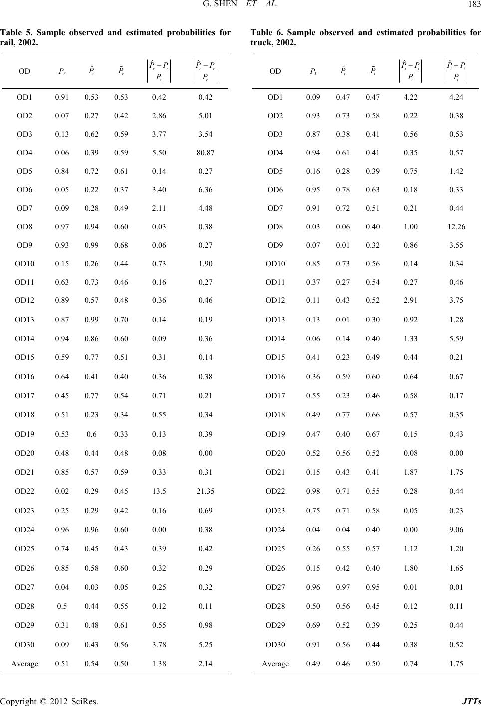

G. SHEN ET AL. 183
Table 6. Sample observed and estimated probabilities for
truck, 2002.
OD Pt
Table 5. Sample observed and estimated probabilities for
rail, 2002.
OD Pr ˆr P r P
 ˆrr
r
PP
P
 ˆrr
r
PP
P

OD1 0.91 0.53 0.53 0.42 0.42
OD2 0.07 0.27 0.42 2.86 5.01
OD3 0.13 0.62 0.59 3.77 3.54
OD4 0.06 0.39 0.59 5.50 80.87
OD5 0.84 0.72 0.61 0.14 0.27
OD6 0.05 0.22 0.37 3.40 6.36
OD7 0.09 0.28 0.49 2.11 4.48
OD8 0.97 0.94 0.60 0.03 0.38
OD9 0.93 0.99 0.68 0.06 0.27
OD10 0.15 0.26 0.44 0.73 1.90
OD11 0.63 0.73 0.46 0.16 0.27
OD12 0.89 0.57 0.48 0.36 0.46
OD13 0.87 0.99 0.70 0.14 0.19
OD14 0.94 0.86 0.60 0.09 0.36
OD15 0.59 0.77 0.51 0.31 0.14
OD16 0.64 0.41 0.40 0.36 0.38
OD17 0.45 0.77 0.54 0.71 0.21
OD18 0.51 0.23 0.34 0.55 0.34
OD19 0.53 0.6 0.33 0.13 0.39
OD20 0.48 0.44 0.48 0.08 0.00
OD21 0.85 0.57 0.59 0.33 0.31
OD22 0.02 0.29 0.45 13.5 21.35
OD23 0.25 0.29 0.42 0.16 0.69
OD24 0.96 0.96 0.60 0.00 0.38
OD25 0.74 0.45 0.43 0.39 0.42
OD26 0.85 0.58 0.60 0.32 0.29
OD27 0.04 0.03 0.05 0.25 0.32
OD28 0.5 0.44 0.55 0.12 0.11
OD29 0.31 0.48 0.61 0.55 0.98
OD30 0.09 0.43 0.56 3.78 5.25
Average 0.51 0.54 0.50 1.38 2.14
ˆt
P t P
 ˆtt
t
PP
P
 ˆtt
t
PP
P

OD1 0.09 0.47 0.47 4.22 4.24
OD2 0.93 0.73 0.58 0.22 0.38
OD3 0.87 0.38 0.41 0.56 0.53
OD4 0.94 0.61 0.41 0.35 0.57
OD5 0.16 0.28 0.39 0.75 1.42
OD6 0.95 0.78 0.63 0.18 0.33
OD7 0.91 0.72 0.51 0.21 0.44
OD8 0.03 0.06 0.40 1.00 12.26
OD9 0.07 0.01 0.32 0.86 3.55
OD10 0.85 0.73 0.56 0.14 0.34
OD11 0.37 0.27 0.54 0.27 0.46
OD12 0.11 0.43 0.52 2.91 3.75
OD13 0.13 0.01 0.30 0.92 1.28
OD14 0.06 0.14 0.40 1.33 5.59
OD15 0.41 0.23 0.49 0.44 0.21
OD16 0.36 0.59 0.60 0.64 0.67
0.46 0.58 0.17
0.57 0.35
OD17 0.55 0.23
OD18 0.49 0.77 0.66
OD19 0.47 0.40 0.67 0.15 0.43
OD20 0.52 0.56 0.52 0.08 0.00
OD21 0.15 0.43 0.41 1.87 1.75
OD22 0.98 0.71 0.55 0.28 0.44
OD23 0.75 0.71 0.58 0.05 0.23
OD24 0.04 0.04 0.40 0.00 9.06
OD25 0.26 0.55 0.57 1.12 1.20
OD26 0.15 0.42 0.40 1.80 1.65
OD27 0.96 0.97 0.95 0.01 0.01
OD28 0.50 0.56 0.45 0.12 0.11
OD29 0.69 0.52 0.39 0.25 0.44
OD30 0.91 0.56 0.44 0.38 0.52
Average 0.49 0.46 0.50 0.74 1.75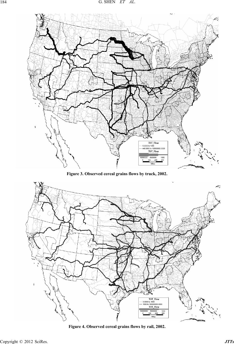

G. SHEN ET AL. 184
Fig Obserereal grainsy tr20
ure 3.ved c flows buck, 02.
Figure 4. Observed cereal grains flows by rail, 2002.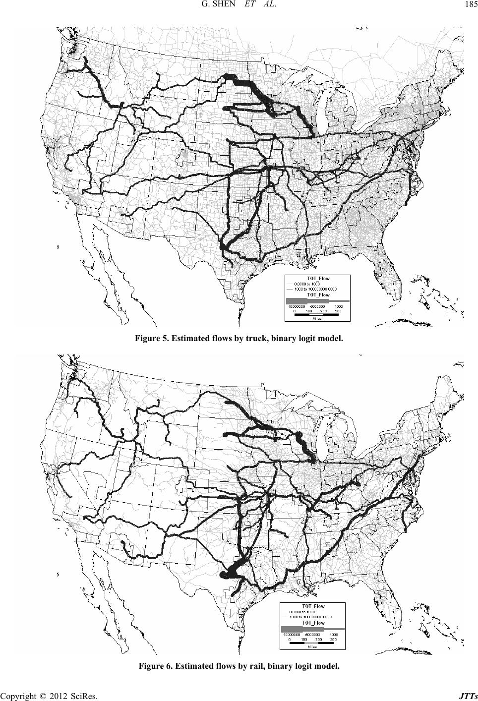

G. SHEN ET AL. 185
Figure 5. Estimated flows by truck, binary logit model.
Figure 6. Estimated flows by rail, binary logit model.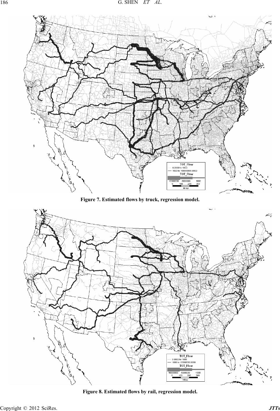

G. SHEN ET AL. 186
Figure 7. Estimated flows by truck, regression model.
Figure 8. Estimated flows by rail, regression model.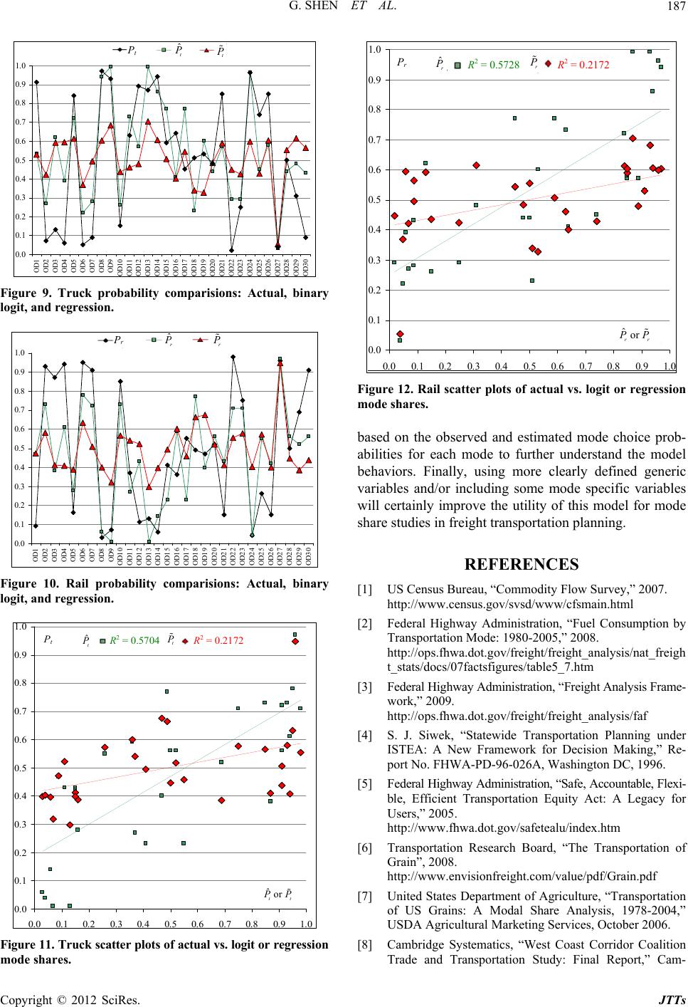

G. SHEN ET AL. 187
0. 0
0. 1
0. 2
0. 3
0. 4
0. 5
0. 6
0. 7
0. 8
0. 9
1. 0
OD1 OD2 OD3 OD4 OD5 OD6 OD7 OD8 OD9
O
D10
O
D11
O
D12
O
D13
O
D14
O
D15
O
D16
O
D17
O
D18
O
D19
O
D20
O
D21
O
D22
O
D23
O
D24
O
D25
O
D26
O
D27
O
D28
O
D29
O
D30
系列2系列3系列1
ˆt
P
P
t
t
P

0. 0
0. 1
0. 2
0. 3
0. 4
0. 5
0. 6
0. 7
0. 8
0. 9
1. 0
0. 0
0.
1
0.
2
0.3
0.
4
0.5
0. 6
0. 7
0. 8
0. 9
1
.0
ˆr
P
P
r
R
2
= 0.57 28 R
2
= 0.21 72
ˆor
rr
P
P

r
P

Figure 9. Truck probability comparisions: Actual, binary
logit, and regression.
0. 0
0. 1
0. 2
0. 3
0. 4
0. 5
0. 6
0. 7
0. 8
0. 9
1. 0
OD1 OD2 OD3 OD4 OD5 OD6 OD7 OD8 OD9
OD1 0 OD1 1 OD1 2 OD1 3 OD1 4 OD1 5 OD1 6 OD1 7 OD1 8 OD1 9 OD2 0 OD2 1 OD2 2 OD2 3 OD2 4 OD2 5 OD2 6 OD2 7 OD2 8 OD2 9 OD3 0
系列
1
系列
2
系列
3
ˆr
P
P
r
r
P

Figure 12. Rail scatter plots of actual vs. logit or regression
mode shares.
based on the observed and estimated mode choice prob-
abilities for each mode to further understand the model
behaviors. Finally, using more clearly defined generic
ng some mode specific variables
will certainly improve the utility of this model for mode
share studies in freight transportation planning.
REFERENCES
[1] US Census Bureau, “Commodity Flow Survey,” 2007.
http://www.census.gov/svsd/www/cfsmain.html
[2] Federal Highway Administration, “Fuel Consumption by
Transportation Mode: 1980-2005,” 2008.
http://ops.fhwa.dot.gov/freight/freight_analysis/nat_freigh
t_stats/docs/07factsfigures/table5_7.htm
[3] Federal Highway Administration, “Freight Analysis Frame-
work,” 2009.
http://ops.fhwa.dot.gov/freight/freight_analysis/faf
[4] S. J. Siwek, “Statewide Transportation Planning under
ISTEA: A New Framework for Decision Making,” Re-
port No. FHWA-PD-96-026A, Washington DC, 1996.
[5] Federal Highway Administration, “Safe, Accountable, Flexi-
ble, Efficient Transportation Equity Act: A Legacy for
Users,” 2005.
http://www.fhwa.dot.gov/safetealu/index.htm
[6] Transportation Research Board, “The Transportation of
Grain”, 2008.
http://www.envisionfreight.com/value/pdf/Grain.pdf
[7] United States Department of Agriculture, “Transportation
of US Grains: A Modal Share Analysis, 1978-2004,”
USDA Agricultural Marketing Services, October 2006.
[8] Cambridge Systematics, “West Coast Corridor Coal
rtation Study: Final Report,” Cam-
variables and/or includi
Figure 10. Rail probability comparisions: Actual, binary
logit, and regression.
0. 0
0. 1
0. 2
0. 3
0. 4
0. 5
0. 6
0. 7
0. 8
0. 9
1. 0
0.00.1 0.20.3 0.40.5 0.60.7 0.80.9 1.0
系列1系列2
ˆt
P
P
t
t
P

R
2
= 0.5704 R
2
= 0.2172
ˆor
tt
PP

ition
Figure 11. Truck scatter pl ots of actual v s. logit or regressi on
mode shares. Trade and Transpo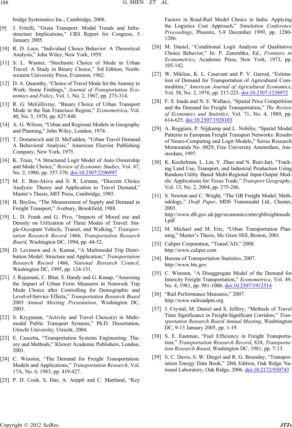

G. SHEN ET AL. 188
bridge Systematics Inc., Cambridge, 2008.
[9] J. Fritelli, “Grain Transport: Modal Trends and Infra-
structure Implications,” CRS Report for Congress, 5
January 2005.
[10] R. D. Luce, “Individual Choice Behavior: A Theoretical
Analysis,” John Wiley, New York, 1959.
[11] S. L. Warner, “Stochastic Choice of Mode in Urban
Travel: A Study in Binary Choice,” 3rd Edition, North-
western University Press, Evanston, 1962.
[12] D. A. Quarmby, “Choice of Travel Mode for the Journey to
Work: Some Findings,” Journal of Transportation Eco-
nomics and Policy, Vol. 1, No. 2, 1967, pp. 273-314.
[13] R. G. McGillivray, “Binary Choice of Urban Transport
Mode in the San Francisco Region,” Econometrica, Vol.
40, No. 5, 1970, pp. 827-848.
hn Wiley, London, 1974.
5] T. Domencich and D. McFadden, “Urban Travel Demand:
A Behavioral Analysis,” American Elsevier Publishing
Company, New York, 1975.
[16] K. Train, “A Structured Logit Model of Auto Ownership
and Mode Choice,” Review of Economic Studies, Vol. 47,
No. 2, 1980, pp. 357-370. doi:10.2307/2296997
[14] A. G. Wilson, “Urban and Regional Models in Geography
and Planning,” Jo
[1
[17] M. E. Ben-Akiva and S. R. Lerman, “Discrete Choice
Analysis: Theory and Application to Travel Demand,”
Master’s Thesis, MIT Press, Cambridge, 1985.
[18] B. Bayliss, “The Measurement of Supply and Demand in
Freight Transport,” Avebury, Brookfield, 1988.
[19] L. D. Frank and G. Pivo, “Impacts of Mixed use and
Density on Utilization of Three Modes of Travel: Sin-
gle-Occupant Vehicle, Transit, and Walking,” Transpor-
tation Research Record 1466, Transportation Research
Board, Washington DC, 1994, pp. 44-52.
ucture and Application,” Transportation
Research Record 1466, National Research Council
Washington DC, 1995, pp. 124
[21] J. Rajamani, C. Bhat, S. Handy and G. Knaap, “Assessing
the Impact of Urban Form Measures in Nonwork Trip
Mode Choice after Controlling for Demographic
Level-of-Service Effects,” Transportation Research Board
2003 Annual Meeting Presentation, Washington DC,
2003.
[22] S. Krygsman, “Activity and Travel Choice(s) in Multi-
modal Public Transport Systems,” Ph.D. Dissertation,
Utrecht University, Utrecht, 2004.
[23] E. Cascetta, “Transportation Systems Engineering: Th
ory and Methods,” Kluwer Academic Publishers, London,
2001.
[24] C. Winston, “The Demand for Freight Transportation
Models and Applications,” Transportation Research, Vol
17A, No. 6, 1983, pp. 419-427.
[25] P. D. Cook, S. Das, A. Aeppli and C. Martland, “Key
Factors in Road-Rail Model Choice in India: Applying
the Logistics Cost Approach,” Conference
Proceedings, Phoenix, 5-8 December 1999, pp. 1280-
1286.
[26] M. Daniel, “Conditional Logit Analysis of Qualitative
Choice Behavior,” In: P. Zarembka, Ed., Frontiers in
Econometrics, Academic Press, New York, 1973, pp.
105-142.
[27] W. Miklius, K. L. Casavant and P. V. Garrod, “Estima-
tion of Demand for Transportation of Agricultural Com-
modities,” American Journal of Agricultural Economics,
Vol. 58, No. 2, 1976, pp. 217-223. doi:10.2307/1238972
[20] D. Levinson and A. Kumar, “A Multimodal Trip Distri-
bution Model: Str,
-131.
Simulation
[28] F. S. Inada and N. E. Wallace, “Spatial Price Competition
and the Demand for Freight Transportation,” The Review
of Economics and Statistics, Vol. 71, No. 4, 1989, pp.
614-625. doi:10.2307/1928103
[29] A. Reggiani, P. Nijjkamp and L. Nobilio, “Spatial Modal
Patterns in European Freight Transport Networks: Results
of Neuro-Computing and Logit Models,” Series Research
Memoranda No. 0029, Free University Amsterdam, Am-
sterdam, 1997.
tility Based Multi-Regional Input-Output Mod-
[32] M. Michael and M. Eric, “Urban Transportation Plan-
ning,” Master’Boston, 2001.
[33] Caliper Corpor8.
2514
and
e-
:
.
[30] K. Kockelman, L. Lin, Y. Zhao and N. Ruiz-Juri, “Track-
ing Land Use, Transport, and Industrial Production Using
Random-U
els: Applications for Texas Trade,” Transport Geography,
Vol. 13, No. 2, 2004, pp. 275-286.
[31] S. Newton and C. Wright, “The GB Freight Model: Meth-
odology,” Draft Paper, MDS Transmodal Ltd., Chester,
2003.
http://www.dft.gov.uk/pgr/economics/ntm/gbfreightmode
l.pdf
s Thesis, Mc Graw Hill,
ation, “TransCAD,” 200
http://www.caliper.com
[34] Bureau of Transportation Statistics, 2007.
http://www.bts.gov
[35] C. Winston, “A Disaggregate Model of the Demand for
Intercity Freight Transportation,” Econometrica, Vol. 49,
No. 4, 1981, pp. 981-1006. doi:10.2307/191
7-13.
3
[36] “Rail Performance Measures,” 2007.
http://www.railroadpm.org
[37] J. Crystal, M. Daniel and S. Jeffery, “Methods of Travel
Time Significance in Freight-Significant Corridors,” Tran-
sportation Research Board Annual Meeting, Washtington
DC, 9-13 January 2005, pp. 1-19.
[38] S. E. Eastman, “Fuel Efficiency in Freight Transporta-
tion,” Transportation Research Record, 824, Transporta-
tion Research Board, Washington DC, 1981, pp.
[39] S. C. Davis, S. W. Diegel and R. G. Bounday, “Transpor-
tation Energy Data Book,” 28th Edition, Oak Ridge Na-
tional Laboratory, Oak Ridge, 2006. doi:10.2172/93074