A Tight Prediction Interval for False Discovery Proportion under Dependence

doi:10.4236/ojs.2012.22018

Paper Menu >>

Journal Menu >>

Open Journal of Statistics, 2012, 2, 163-171

http://dx.doi.org/10.4236/ojs.2012.22018 Published Online April 2012 (http://www.SciRP.org/journal/ojs)

163

A Tight Prediction Interval for

False Discovery Proportion under Dependence

Shulian Shang, Mengling Liu, Yongzhao Shao*

Division of Biostatistics, New York University School of Medicine, New York, USA

Email: *shaoy01@nyu.edu

Received February 1, 2012; revised March 5, 2012; accepted March 16, 2012

ABSTRACT

The false discovery proportion (FDP) is a useful measure of abundance of false positives when a large number of hy-

potheses are being tested simultaneously. Methods for controlling the expected value of the FDP, namely the false dis-

covery rate (FDR), have become widely used. It is highly desired to have an accurate prediction interval for the FDP in

such applications. Some degree of dependence among test statistics exists in almost all applications involving multiple

testing. Methods for constructing tight prediction intervals for the FDP that take account of dependence among test sta-

tistics are of great practical importance. This paper derives a formula for the variance of the FDP and uses it to obtain an

upper prediction interval for the FDP, under some semi-parametric assumptions on dependence among test statistics.

Simulation studies indicate that the proposed formula-based prediction interval has good coverage probability under

commonly assumed weak dependence. The prediction interval is generally more accurate than those obtained from ex-

isting methods. In addition, a permutation-based upper prediction interval for the FDP is provided, which can be useful

when dependence is strong and the number of tests is not too large. The proposed prediction intervals are illustrated

using a prostate cancer dataset.

Keywords: Multiple Testing; False Discovery Proportion; False Discovery Rate; Weak Dependence; Correlated Test

Statistics; High-Dimensional Data Analysis; Prediction Interval; Upper Prediction Bound;

Permutation-Based Method

1. Introduction

When a large number of hypotheses are tested simulta-

neously, a direct measure of the abundance of false posi-

tive findings is the false discovery proportion (FDP),

defined as FDP, or 1





1max ,1RR

, where R denotes the total

number of rejections, V denotes the number of rejections

of true null hypotheses, and . Moti-

vated by various genetic and genomic studies and other

applications, many useful procedures have been proposed

to control the expected value of FDP, namely the false

discovery rate (FDR) [1-5]. Indeed, it is well known that

controlling FDR has power advantages over the tradi-

tional way of controlling family-wise type I error [1,2].

Suppose a study is properly designed to control the FDR

at 5%. If such a study is independently repeated many

times, the average of the FDPs in these repeated studies

can be expected to be no more than 5%. However, for a

particular study (without repetition), the FDP is more

directly relevant than FDR. Therefore, when a study is

designed to control FDR under common designs, it is

still very much desirable to assess FDP, e.g. to construct

a prediction interval for the FDP. One can also consider

designing a study controlling FDP instead of FDR. This

approach has been less successful since FDP is a random

variable and is less straightforward to control than the

FDR. Indeed, researchers have proposed various proce-

dures aimed at controlling the FDP [6-13], from which

confidence envelopes for the FDP can be obtained si-

multaneously for all possible rejection regions. However,

confidence envelopes from the existing FDP controlling

procedures are often too conservative for predicting a

tight range for the FDP. In particular, when weak corre-

lations exist among test statistics, methods for construct-

ing tight prediction interval for the FDP are still limited.

In the multiple testing context, test statistics are often

correlated, e.g. in microarray experiments and functional

magnetic resonance imaging, correlations arise due to

biological, spatial, temporal or technical factors. A major

challenge for predicting FDP is to account for unknown

correlations between test statistics. It has been shown via

numerical studies that when test statistics are correlated,

the variability of FDP can increase dramatically [14-17].

This can also be seen from the variance formula derived

*Corresponding author.

S. SHANG ET AL.

164

in the next section (Formula (2)). Permutation-based me-

thods are often considered in the presence of dependency,

e.g. [15]. Permutation-based methods have several limita-

tions. For instance, they are not applicable when no group

structure (e.g., groups of cases and controls) is present as

in some imaging studies [9]. Additionally, if the purpose

of testing is to detect differences in means, then a per-

mutation-based test can have an inflated Type I error rate

by picking up signals due to unequal variances or skew-

ness of two distributions [18]. Pan [3] and Xie et al. [19]

also pointed out that permutation-based procedures tend

to overestimate FDR. Finally, a permutation-based ap-

proach is generally very computationally intensive; it

often becomes not feasible when the number of tests is

large.

Other works on FDP have been proposed with efforts

to accommodate the correlations among test statistics.

For example, Ge et al. [12,20] proposed a formula for the

upper prediction bound of the FDP assuming that test

statistics under true null hypotheses are independent and

also proposed a permutation algorithm to obtain a simul-

taneous upper prediction band of the FDP. Under the

assumption that p-values are independent or follow a

conditional equicorrelated multivariate normal model,

Roquain and Villers [21] provided exact calculations for

the cumulative distribution function (CDF) and moments

of FDP for the step-up and step-down procedures. Ghosal

and Roy [22] proposed a nonparametric Bayesian proce-

dure to obtain the posterior distribution of FDP under the

intraclass or autoregressive correlation structure. In all

these studies on FDP under dependence, the correlation

among test statistics is either ignored or assumed to fol-

low some parametric models. A flexible semiparametric

approach to modeling dependency among test statistics

has not emerged.

In this paper, we first derive an explicit formula for the

variance of the FDP under a semiparametric weak de-

pendence assumption among the test statistics. The vari-

ance formula is easily interpretable and elucidates the

effect of correlation on the variability of FDP. Using the

variance formula, we obtain an upper prediction interval

for the FDP. This approach is semiparametric in nature

because only the average of the pairwise Pearson correla-

tion between test statistics needs to be estimated. The

formula-based prediction interval is easy to evaluate even

when testing a vast number of hypotheses where no other

methods are computationally feasible. Simulation studies

indicate that the formula-based prediction interval has

good coverage probabilities under weak to moderate de-

pendence. In many situations, as illustrated, the predic-

tion interval is quite short (tight) and generally more ac-

curate than competitors. In addition, we discuss a per-

mutation-based upper prediction interval for FDP which

is useful under strong dependence. We illustrate the pro-

posed prediction intervals using a prostate cancer data-

set.

2. Methods

2.1. Notation

Consider testing m hypotheses simultaneously. Rejec-

tions are made based on p-values, with a fixed rejection

region







for some α. Denote the rejection status of

the ith test by





RIp







, where pi denotes the

p-value of the ith test and





is an indicator function.

Denote the power of the ith test as 1 – βi.

Let V and U be the total number of incorrect and cor-

rect rejections, respectively. The total number of rejec-

tions or discoveries is 1i



. Let M0 denote

the index set of the m0 tests for which null hypotheses are

true and M1 the index set of m1 = m – m0 tests for which

alternative hypotheses are true. The proportion of true



null hypotheses is 0

πm

. When test statistics are de-

pendent, as in [23], we have













Var 11

111,

ij Mij





 



 













corr ,

Vij



0

,ij M for , and

where





ij Mij

Vmm









is the average correlation coeffi-

cient. Similarly, for the correct rejections,











Var 1

11,

Ui ijj

ij Mij

























corr ,

Uij



1

,M for ij . Denote where







. If effect sizes are all equal, i.e.





for all i, we can obtain a simplified formula

















Var111 U

Um m





, where



ij Mij

Umm









. Additionally, let













corr ,

UVi j



1

M0

jM for i, . De-



note the average correlation 10

iM jM

UV mm







Under some general regularity conditions including weak

Table 1 summarizes the outcomes of m tests and their

expected values.

2.2. Formula-Based Prediction Interval

2.2.1. De rivation of Predicti on I n t erval

S. SHANG ET AL. 165

Table 1. Outcome and expected outcome of testing m hypo-

theses.

Outcome

Reject H0 Accept H0 Total

H0 is true V m0 – V m0

H1 is true U m1 – U m1

Total R m – R m

Expected Outcome

Reject H0 Accept H0 Total

H0 is true m0α



01m



 m0

H1 is true







 1



Total



1mm









1mm





 m

dependence among test statistics, Farcomeni [24] proved

that the FDP,







,0,1











, as a stochastic

process indexed by α, is an asymptotically Gaussian

process (see Theorem 2 of [24]). In particular, for a fixed

α, the FDP has an asymptotically normal distribution

under weak dependence as discussed in Farcomeni [24].

More specifically, assuming that 0

0π1, when test

statistics are independent or weaklyt, depend0



,



 and 0



 as m, we show tP

a Normutiontotically with special

mean and variance (see Appendix A (A.1)). No assump-

tions about higher-order correlation terms are required.

When effect sizes are all equal, explicit forms for the

hat FD

follows al diasym

strib p

ean







and variance







of the FDP can be

easily ed using the delethod and are given by obtainta m





π1π1





 , (1)





π1π







 4

 









, (2)

where



1π

π2π1















 (3)

and

 



 







 







. For a moderate to large sample size n,

ragthe averror e Type II e0



. Then

000

ππ2π

QVUUV

cmm





 









(4)



11



where

π1

1π

π1





 . From (4), it is evident

that when all the test statistics are independent, 2







ly proportional to m; wh

dependent, correlations also contribute to the variance.

inverse en some test statistics are

The rejection threshold α in multiple testing is typally

less than 0.05 and thus ω is small, making the last two

terms of (4) small. The average correlation among true

null test statistics, which is represented by V



, can have

a large influence on the variance of FDP.

When all the parameters are known, a prediction in-

terval could be derived based on the asympic distribu-

tion of FDP. We shall discuss the estimat

tot

ion of parame-

ters in details next section. In multiple testing we are

primarily concerned about high FDPs so an upper predic-

tion interval is of interest. A



1001



% upper predic-

tion interval for FDP is given by 0,QQ













, where



is the





1001





th quantile ostandard normal

distribution.

f the

ice, the distrib

FDP under dependenc

ch as the log-transformation to be practi-

With finite sample size in practution of

e is often skewed, suggesting trans-

formations su

lly useful. Moreover, by the delta method (see Appen-

dix A for more details), when the FDP is asymptotically

normal, Y = log(FDP) is also asymptotically normal, i.e.,









asymptotically, where formulas for Y



and 2



are derived in Appendix A (A.2). Thus it is not

surprising that Y = log(FDP) is closer to normal than the

FDP itself, part

ima



icularly under weak dependence. The ap-

proxte mean and variance of Y are:







loglog π1π



















 









(5)





00 0

1π11

ππ 1π1





 







 

where

(6)



is in (3). Applying the expone

mation, a

ntial transfor-





1001





% upper prediction interval for the

FDP can be constructed as





0, expz





.

tion

sed prediction interv





2.2.2. Estima

To calculate the formula-baal







0, expz











, we need to estimate necessary pa-

rameters in Y



and Y



first. We adopt the estimator

π proposed for by Storey [2]:















for







0,1



the choice of 0.5 with



. We use t he

odmeth of moment to estimate



. Because









1ER mm





, plugging in the estimate of

he o of rej



πand tbserved total numberections R, we

hae 0

ˆ1Rm

1πm







 The resulting estimator ˆQ



.

S. SHANG ET AL.

166

essentially the same as the FDR estimator proposed by

Storey [2]: 0

ˆQ





er

. However, the objective he is

to obtain a predictive interval or equivalently an upper

bound for FDP sinwe mainly care about large values

of FDP.

The correlation



between the ith and jth rejection

indicators is

 



Var Var

iji j

ER RERER





 









We here consider one-sided z-test for two-group com-

parison to illustrate the estimation of correlation. Two-

sided z-test and t-test are given in Appendix B. Follow-



.

ing the notation defined in Section 2.1, we have











 

, (7)















, (8)









 

 



where Ψ is the CDF of the standard bivariate normal dis-

tribution, and ρij denotes the Pearson correlati

the ith and jth test statistics. We propose the following





, (9)

on between

procedure to estimate the average correlations. In prac-

tice, when m is very large (m > 2000), we propose to run

the procedure on a random subset of m tests to save

computation time.

1) Estimate the correlations between test statistics ρij

using the sample correlations. As in [25], an empirical

Bayes shrinkage estimator of sample correlations can be

used.

2) For the ith test with z-score zi, estimate the condi-

tional probability of the corresponding hypothesis being

a true alternative hypothesis:







1π

1ππ

iz i

PiM zzz



 







where





is the density of



0,1N and function



is the mean of z-scoreshe alternative hy-

pothesis is true. Frome esti

when t

mate ˆ



we can get

1ˆ



ˆzz







 .

3) Predict whether the tests belong to M1 or M0 by

generating Bernoulli random variables with the estimated

probability





vercorrelations



PiM z.

ntity4) After the ide of each test is predicted, the cor-

ation θij between any two rejection indicators can be

calculated from Formulae (7)-(9).

5) Estimate the aage

rel

, UV



and



using the respective sample means of pairwise cor-

relations.

6) Repeat steps 3 to 5 for a few times, and take the av-

ern

tation-Based Prediction Interval

iction

The

not

age of these estimates of average correlatios.

2.3. Permu

The permutation-based procedure proposed by Korn et al.

[6,7] can be adapted to construct an upper pred

interval for the FDP under general dependence.

method can be expected to be robust because it does

depend on parametric or weak dependence assumptions,

but it requires very intensive computation which may not

be feasible for testing a very large number of hypotheses.

Let n1 and n2 be the sample sizes of the two groups and

suppose that unpaired t-test is performed. First, permute

the group labels and calculate the two-sample t-statistic

p-values for all m tests under the permutated labels. If the

number of possible permutations



 is too large,

perform w = 500 or 1000 random permutations. Second,

for each permutation, order the p-vllest to alues from sma

largest. Let

 

,,,

pp p denordered p-val- te the o

ues for the jth permutation, 1, 2,,jw. Write the

ordered p-values in a wm



matrix:

 

 

 

www

pp p













Third, order the p-values within each comn and put the

smallest p-values on top. Denote the reslting matrix by

S, and its element at the jth row and lth column by

 

p

  







where 1, 2,,jw and 1, 2,,lm.



To construct a





1001





% upper prediction interval

for the FDP, we first find an upper bound V

 for V. Find

the [γw]th row of the matrix S where [a] denotes

closest ller than o

the

integer smar equal to a. The upper

bo estimatedund for V can be as:









VIS











. By construction

SSS



 for 1, 2,,jw



. Using Korn’s con-

trolling procedure,







is the threshold for at most

k false discoveries with 1ce, k is the -γ probability. Hen





1001% uppund for V er boat threshold











Given a rejection region







, the definition of









implies that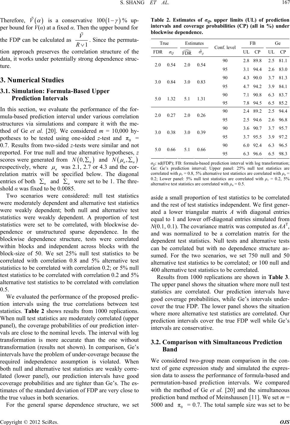





















. Then





 













11PV VPV













.



S. SHANG ET AL. 167





VTherefore,



 is a c



0 1onservative 10



% up-

r V(α) at a er bound for

the FDP can be calculated as

per bound fo the uppfixed α. Then

R



. Since the perma-

ch pre

ediction Intervals

the performance of the for-

orrelation

the me-

thod considered m = 10,000 hy-

tion approaserves the correlation structure of the

data, it works under potentially strong dependence struc-

ture.

3. Numerical Studies

3.1. Simulation: Formula-Based Upper

In this section, we evaluate

mula-based prediction interval under various c

structures via simulations and compare it with

of Ge et al. [20]. We

potheses to be tested using one-sided z-test and 0

π =

0.7. Results from two-sided z-tests were similar and not

reported. For true null and true alternative hypotheses, z

scores were generated from



0, n

N and









respectively, where a



was 2.1, 2.7 or 4.3 and the cor-

relation matrix will be specified below. The diagonal

entries of both n

 and a

 were set to be 1. The thre-

shold α was fixed to be 0.0085

Two scenarios were considered: null test statistics

were moderately dependent and alternative test statistics

were weakly de endent; both null and alternative test

statistics were weakly dependent. A proportion of test

FB Ge

atistics were set to be correlated, with blockwise de-

pendence or unstructured sparse dependence. In the

blockwise dependence structure, tests were correlated

within blocks and independent across blocks with the

block-size of 50. We set 25% null test statistics to be

correlated with correlation 0.8 and 5% alternative test

statistics to be correlated with correlation 0.2; or 5% null

test statistics to be correlated with correlation 0.2 and 5%

alternative test statistics to be correlated with correlation

0.5.

We evaluated the performance of the proposed predic-

tion intervals using the true correlations between test

statistics. Table 2 shows results from 1000 replications.

When null test statistics are moderately correlated (upper

panel), the coverage probabilities of our prediction inter-

vals are close to the nominal levels. The interval with log

transformation is more accurate than the one without

transformation (results not shown). In comparison, Ge’s

intervals have the problem of under-coverage because the

required independence assumption is violated. When

both null and alternative test statistics are weakly corre-

lated (lower panel), our prediction intervals have good

coverage probabilities and are tighter than Ge’s. The es-

timates of the standard deviation of FDP are very close to

the true values in both scenarios.

For the general sparse dependence structure, we set

Table 2. Estimates of σQ, upper limits (UL) of prediction

intervals and coverage probabilities (CP) (all in %) under

blockwise dependence .

True Estimates

FDR σQ



FDR Q



Conf. level

UL CP ULCP

90 2.8 89.82.581.1

2.0 0.542.00.5495 3.1 94.42.683.0

90 4.3 .03.7.3

3. 90 81

0 0.843.00.8395 4.7 94.23.984.1

90 7.1 90.86.383.7

5.0 1.325.11.3195 7.8 94.56.585.2

90 2.4 89.22.594.4

2.0 0.272.00.2695 2.5 94.62.696.8

90 3.6 90.73.795.7

3.0 0.383.00.3995 3.7 95.53.997.2

90 6.0 92.46.396.5

5.0 0.665.10.6695 6.3 96.66.598.3

σQ: sd(FDP); FB: formula-based predicintervaram

Gedictin Upper l: 25% ll tice

correlated with ρv = 0.8, 5% alternativetatistiati

0.2; Lower panel: 5% null test statistire corρ.

alti stas alated ρu = 0.

s simulated from

N(0.1, 0.1). The covariance matrix was computed as AAT,

e situation

y and simulated the expres-

withthod of Ge et al. [20] and the simultaneous

tion l with log tnsforation;

e: G’s preion terval;pane

test s

cs are

est sta

correl

tist

ed w

s ar

th ρu =

cs a

with

related with

v = 02, 5%

ternave testtisticre corre

aside a small proportion of test statistics to be correlated

and the rest of test statistics independent. We first gener-

ated a lower triangular matrix A with diagonal entries

equal to 1 and lower off-diagonal entrie

and was normalized to be a correlation matrix for the

dependent test statistics. Null tests and alternative tests

can be correlated but with no dependence structure as-

sumed. For the two scenarios, we set 750 null and 50

alternative test statistics to be correlated; or 100 null and

400 alternative test statistics to be correlated.

Results from 1000 replications are shown in Table 3.

The upper panel shows the situation where more null test

statistics are correlated. Our prediction intervals have

good coverage probabilities, while Ge’s intervals under-

cover the true FDP. The lower panel shows th

here more alternative test statistics are correlated. Our

prediction intervals cover the true FDP well while Ge’s

intervals are conservative.

3.2. Comparison with Simultaneous Prediction

Band

We considered two-group mean comparison in the con-

text of gene expression stud

sion data to assess the performance of formula-based an

permutation-based prediction intervals. We compare

the me

prediction band method of Meinshausen [11]. We set m =

5000 and 0

π = 0.7. The total sample size was set to be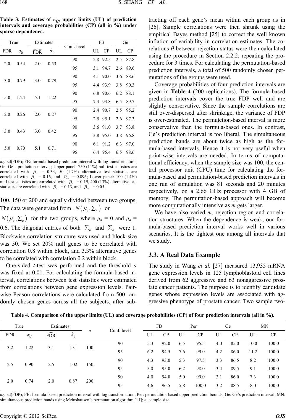

S. SHANG ET AL.

168

Table 3. Estimates of σQ, upper limits (UL) of prediction

intervals and coverage probabilities (CP) (all in %) under

sparse dependenc e.

True Estimates FB Ge

FDR σ



FDR Q



Conf. level

UL CP ULCP

90 2.8 92.5 2.587.8

2.0 0.54 2.0 0.53 95 3.1 94.7 2.689.6

90 4.1 .0 3.6.6

3.0 0.79 90 88

3.0 0.7995 4.4 93.9 3.890.3

90 6.8 90.6 6.288.1

5.0 1.24 5.1 1.22 95 7.4 93.8 6.589.7

90 2.4 90.7 2.595.2

2.0 0.26 2.0 0.27 95 2.5 95.1 2.697.3

90 3.6 91.0 3.793.8

3.0 0.43 3.0 0.42 95 3.8 95.0 3.896.8

90 6.1 91.2 6.397.0

5.0 0.70 5.1 0.71 95 6.4 95.4 6.598.6

σQ: sd(FDP); FB: formula-based predictntervalm;

G’rvr pane50 (11%utice

ted with

ion i

l: 7

with

) n

log tra

ll test sta

nsfor

tis

ation

s are: Ge

rrela

s prediction inteal; Uppe

co v



= 0.33, 50 (1.lternasi

rrelated with

7%) ative test tatistcs are

co u



= 0.16, and uv



096; L:)

t rreith

= 0.ower panel 100 (1.4%

null tesstatistics are colated wv



= 0.19, 4t

s i

00 (13%) al ernative test

statistic are correlated w th u



= 0.13, anduv



0.6. The diagonn

 and a

 were 1.

es to be correlated with

correlation

to be correl

anthr

ran-

The formula-based

ur for-

l Data Example

measured 13,935 mRNA

ymphoblastoid cell lines

FB Per Ge MN

= 0.05.

100, 150 or 200 and equally divided between two groups.

The data wereenerated from





 or





 for the two gros, where μn = 0 and μa = u

al entries of both

Blockwise correlation structure was used and block-size

was 50. We set 20% null gen

0.8 within block, and 3.3% alternative genes

ated with correlation 0.2 within block.

One-sided t-test was performedd the eshold α

was fixed at 0.01. For calculating the formula-based in-

terval, correlations between test statistics were estimated

from correlations between gene expression levels. Pair-

wise Peason correlations were calculated from 500

mly chosen genes across all the subjects, after sub-

tracting off each gene’s mean within each group as in

[26]. Sample correlations were then shrunk using the

Table 4. Comparison of the upper limits (UL) and covera

True Estimates

empirical Bayes method [25] to correct the well known

inflation of variability in correlation estimates. The co-

relations θ between rejection status were then calculated

using the procedure in Section 2.2.2, repeating the pro-

cedure for 3 times. For calculating the permutation-based

prediction intervals, a total of 500 randomly chosen per-

mutations of the groups were used.

Coverage probabilities of four prediction intervals are

given in Table 4 (200 replications).

ediction intervals cover the true FDP well and are

slightly conservative. Since the sample correlations are

still over-dispersed after shrinkage, the variance of FDP

is over-estimated. The permutetion-based interval is more

conservative than the formula-based ones. In contrast,

Ge’s prediction interval is too liberal. The simultaneous

prediction bands are about twice as high as the for-

mula-based intervals. Hence it is not very useful when

point-wise intervals are needed. In terms of computa-

tional efficiency, when the sample size was 100, the cen-

tral processor unit (CPU) time for calculating the for-

mula-based and permutation-based prediction intervals in

one run of simulation was 81 seconds and 20 minutes

respectively, on a 2.66 GHz processor with 4 GB of

memory. The permutation-based approach will become

more computationally intensive as m gets larger.

We have also varied m, rejection region and correla-

tion structures. When the dependence is weak, o

ula-based prediction interval works well in various

scenarios. It is the tightest one among all intervals that

we study.

3.3. A Rea

The study in Wang et al. [27]

gene expression levels in 125 l

derived from 62 aggressive and 63 nonaggressive pros-

tate cancer patients. The purpose is to identify candidate

genes whose expression levels are associated with ag-

gressive phenotype of prostate cancer. Two sample two-

probabilities (CP) of four prediction intervals (all in %).

FDR σQ



FDR ˆQ



UL CP ULCP UL CP UL CP

n Conf. level

90 5.392.0 6.595.5 4.0 85.0 10.0 100.0

3.2 1.22 3.31 100 6.2 7.6 4.2 86.0 11.2

90 100.0

2.5 0.90 2.5 1.02 150

2.0 0.74 2.0 0.87 200 100.0

.1 195 94.5 99.0 100.0

4.393.0 5.397.5 3.3 86.5 8.2

95 5.095.0 6.298.0 3.4 89.5 9.1 100.0

90 4.094.0 5.099.0 3.1 86.0 7.3 100.0

95 4.696.5 5.83.2 88.5 8.0 100.0

σQ: sd(FDP); FB: formula-based prediction interval with log transation; Per: peutatiosed upr prebounepred inte:

simultaneous prediction bands using Meinshausen’s permutation algorithm [11]; n: sample size.

formrmn-bapediction ds; G: Ge’s ictionrval; MN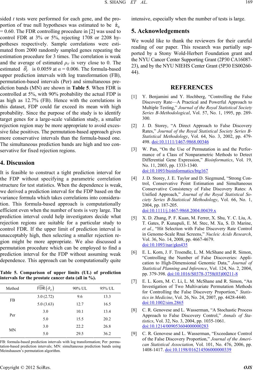

S. SHANG ET AL. 169

sid tesre prmedeane, andpro-

portion of null htheses was estimted to be 0

the

ed tts we

true

erfo

ypo

for ch ge the

= 0.60. The FDR controlling procedure in [2] was used to

ontrol FDR at 3% or 5%, rejecting 1708 or 2208 hy- c

potheses respectively. Sample correlations were esti-

mated from 2000 randomly sampled genes repeating

estimation procedure for 3 times. The correlation is weak

and the average of estimated ρV is very close to 0. The

estimated V



is 0.0059 at α = 0.006. The formula-based

upper prediction intervals with log transformation (FB),

permutation-based intervals (Per) and simultaneous pre-

diction bands (MN) are shown in Tabl e 5. When FDR is

controlled at 5%, with 90% probability the actual FDP is

as high as 12.7% (FB). Hence with the correlations in

this dataset, FDP could far exceed its mean with high

probability. Since the purpose of the study is to identify

target genes for a large-scale validation study, a smaller

rejection region may be more appropriate to avoid exces-

sive false positives. The permutation-based approach gives

more conservative intervals than the formula-based one.

The simultaneous prediction bands are high and too con-

servative for fixed rejection regions.

4. Discussion

It is feasible to construct a tight prediction interval for

the FDP without specifying a parametric correlati

tatistics. When the dependence is

iction interval for the FDP based on the

wstructure for test s

we derived a pred

eak,

variance formula which takes correlations into considera-

tion. This formula-based approach is computationally

efficient even when the number of tests is very large. The

prediction interval could help investigators decide what

rejection regions are suitable for a particular study to

control FDR. If the upper limit of prediction interval is

unacceptably high, then selecting a smaller rejection re-

gion might be more appropriate. We also discussed a

permutation procedure which can be employed to find a

prediction interval for the FDP without assuming weak

dependence. This approach can be computationally quite

Table 5. Comparison of upper limits (UL) of prediction

intervals for the prostate cancer data (all in %).

Method





FDR ˆQ



90% UL 95% UL

3.0 (2.72) 9.6 13.3

FB 5.0 (3.63) 12.7 16.5

3.0

10.1 13.4

Per 5.0 15.5 20.2

3.0 22.2

5.0 29.5

26.8

36.2

FB: foa-based predictirvals with log tormation; Pe

tation-based prediction intMN: simultanrediction sing

Meinshausen’s permutation algorithm.

esially tumf tis l

thank the reviewers for their careful

read of our paphis research was partia

ported by a Stony ld-Herbert Fation gand

NCES

tes,” Journal of the Royal Statistical Society Series B-

Statistical Methodology, Vol. 64, No. 3, 2002, pp. 479-

498. doi:10.11

rmulon inte

ervals;

ransf

eous p

r: pe

bands u

rmu-

intensive, pec whenhe nber oests arge.

5. Acknowledgements

We would like to

ing er. Tlly sup-

Wooundrant

the NYU Cancer Center Supporting Grant (2P30 CA16087-

23), and by the NYU NIEHS Center Grant (5P30 ES00260-

44).

REFERE

[1] Y. Benjamini and Y. Hochberg, “Controlling the False

Discovery Rate—A Practical and Powerful Approach to

Multiple Testing,” Journal of the Royal Statistical Society

Series B-Methodological, Vol. 57, No. 1, 1995, pp. 289-

300.

[2] J. D. Storey, “A Direct Approach to False Discovery

11/1467-9868.00346

e Use of Permutation[3] W. Pan, “On th in and the Perfor-

mance of a Class of Nonparametric Methods to Detect

Differential Gene Expression,” Bioinformatics, Vol. 19,

No. 11, 2003, pp. 1333-1340.

doi:10.1093/bioinformatics/btg167

[4] J. D. Storey, J. E. Taylor and D. Siegmund, “Strong Con-

gy, Vol. 66, No. 1,

trol, Conservative Point Estimation and Simultaneous

Conservative Consistency of False Discovery Rates: A

Unified Approach,” Journal of the Royal Statistical So-

ciety Series B-Statistical Methodolo

2004, pp. 187-205.

doi:10.1111/j.1467-9868.2004.00439.x

[5] X. D. Zhang, P. F. Kuan, M. Ferrer, X. Shu, Y. C. Liu, A.

T. Gates, P. Kunapuli, E. M. S

et al., “Hit Selection with False Di

tec, M. Xu, S. D. Marine,

scovery Rate Control

in Genome-Scale Rnai Screens,” Nucleic Acids Research,

Vol. 36, No. 14, 2008, pp. 4667-4679.

doi:10.1093/nar/gkn435

[6] E. L. Korn, J. F. Troendle, L. M. McShane and R. Simon,

“Controlling the Number of False Discoveries: Appli-

cation to High-Dime

Statistical Planning and Inference, Vol.

nsional Genomic Data,” Journal of

124, No. 2, 2004,

pp. 379-398. doi:10.1016/S0378-3758(03)00211-8

[7] E. L. Korn, M. C. Li, L. M. McShane and R. Simon, “An

Investigation of Two Multivariate Permutation Methods

for Controlling the False Discovery Proportion,” Statis-

tics in Medicine, Vol. 26, No. 24, 2007, pp. 4428-4440.

doi:10.1002/sim.2865

[8] C. R. Genovese and L. Wasserman, “A Stochastic Process

Approach to False Discovery Control,” Annals of Sta-

tistics, Vol. 32, No. 3, 2004, pp. 1035-1061.

doi:10.1214/009053604000000283

[9] C. R. Genovese and L. Wasserman, “Exceedance Control

of the False Discovery Proportion,” Journal of the Ameri-

can Statistical Association, Vol. 101, No. 476, 2006, pp.

1408-1417. doi:10.1198/016214506000000339

S. SHANG ET AL.

170

[10] M. J. van der Laan, S. Dudoit and K. S. Pollard, “Aug-

mentation Procedures

for Control of the Generalized

Family-Wise Error Rate and Tail Probabilities for the

Proportion of False Positives,” Statistical Applications in

Genetics and Molecular Biology, Vol. 3, No. 1, 2004,

Article 15.

[11] N. Meinshausen, “False Discovery Control for Multiple

Tests of Association under General Dependence,” Scandi-

navian Journal of Statistics, Vol. 33, No. 2, 2006, pp.

227-237. doi:10.1111/j.1467-9469.2005.00488.x

[12] Y. C. Ge, S. C. Sealfon and T. P. Speed, “Multiple

Testing and Its Applications to Microarrays,” Statistical

Methods in Medical Research, Vol. 18, No. 6, 2009, pp.

543-563. doi:10.1177/0962280209351899

[13] A. Farcomeni, “Generalized Augmentation to Control the

False Discovery Exceedance in Multiple Testing,” Scan-

isc o -

dence,” Bioin-

dinavian Journal of Statistics, Vol. 36, No. 3, 2009, pp.

501-517.

[14] Q. Yang, J. Cui, I. Chazaro, L. A. Cupples and S.

Demissie, “Power and Type I Error Rate of False D

very Rate Approaches in Genome-Wide Association Stu-

die,” BMC Genetics, Vol. 6, Suppl. 1, 2005.

[15] Y. Pawitan, S. Calza and A. Ploner, “Estimation of False

Discovery Proportion under General Depen

formatics, Vol. 22, No. 24, 2006, pp. 3025-3031.

doi:10.1093/bioinformatics/btl527

[16] R. Heller, “Correlated Z-Values and the Accuracy of

Large-Scale Statistical Estimates Comment,” Journal of

the American Statistical Association, Vol. 105, No. 491,

2010, pp. 1057-1059. doi:10.1198/jasa.2010.tm10240

[17] A. Schwartzman and X. H. Lin, “The Effect of Correlation

in False Discovery Rate Estimation,” Biometrika, Vol. 98,

No. 1, 2011, pp. 199-214. doi:10.1093/biomet/asq075

[18] Y. F. Huang, H. Y. Xu, V. Calian and J. C. Hsu, “To

Permute or Not to Permute,” Bioinformatics, Vol. 2

18, 2006, pp. 2244-2248.

2, No.

doi:10.1093/bioinformatics/btl383

[19] Y. Xie, W. Pan and A. B. Khodursky, “A Note on Using

Permutation-Based False Discovery Rate Estimates to

Compare Different Analysis Methods for Microarray

Data,” Bioinformatics, Vol.

4288.

21, No. 23, 2005, pp. 4280-

ti685doi:10.1093/bioinformatics/b

Least Favorable

[20] Y. C. Ge and X. Li, “Control of the False Discovery

Proportion for Independently Tested Null Hypotheses,”

Journal of Probability and Statistics, 2012, in Press.

[21] E. Roquain and F. Villers, “Exact Calculations for False

Discovery Proportion with Application to

Configurations,” Annals of Statistics, Vol. 39, No. 1, 2011,

pp. 584-612. doi:10.1214/10-AOS847

[22] S. Ghosal and A. Roy, “Predicting False Discovery

Proportion under Dependence,” Journal of the American

Statistical Association, Vol. 106, No. 495, 2011, pp. 1208-

1218. doi:10.1198/jasa.2011.tm10488

[23] Y. Shao and C. H. Tseng, “Sample Size Calculation with

Dependence Adjustment for FDR-Control in Microarray

Studies,” Statistics in Medicine, Vol. 26, No. 23, 2007, pp.

4219-4237. doi:10.1002/sim.2862

[24] A. Farcomeni, “Some Results on the Control of the False

Discovery Rate under Dependence,” Scandinavian Jour-

nal of Statistics, Vol. 34, No. 2, 2007, pp. 275-297.

doi:10.1111/j.1467-9469.2006.00530.x

[25] B. Efron, “Empirical Bayes Estimates for Large-Scale

Prediction Problems,” Journal of the American Statistical

Association, Vol. 104, No. 487, 2009, pp. 1015-1028.

doi:10.1198/jasa.2009.tm08523

[26] B. Efron, “Correlation and Large-Scale Simultaneous Sig-

nificance Testing,” Journal of the American Statistical

Association, Vol. 102, No. 477, 2007, pp. 93-103.

doi:10.1198/016214506000001211

[27] L. Wang, H. Tang, V. Thayanithy, S. Subramanian, A. L.

arch,

Oberg, J. M. Cunningham, J. R. Cerhan, C. J. Steer and S.

N. Thibodeau, “Gene Networks and MicroRNAs Impli-

cated in Aggressive Prostate Cancer,” Cancer Rese

Vol. 69, No. 24, 2009, pp. 9490-949

doi:10.1158/0008-5472.CAN-09-2183

Appendix A. Asymptotic Distribution of

e FDP

.1. Under the general weak dependence assumptions

e FDP is asymptotically normal (e.g. Theorem 2 of

that

asymptotically normal. In particular, we also

[23], when test statistics under H0 are weakly dependent

and

th 0



 as m , the asymptotic normality im-

plies



th 00 0

~π,π1π

mmm

 



















Farcomeni [24]). Thus in this appendix, we assume th

some weak dependence assumption is satisfied so

the FDP is

assume approximate joint normality of V and R. As in

Similarly, when test statistics under H1 are weakly de-

pendent and 0



 as m, asymptotic normality

implies

S. SHANG ET AL. 171



~1π1,

1π





1π

 













 













addition





In, if 0







as m, then

 



Co1 10

 

 as

ptotically uncorrelated.

al distribution, for R

> V > 0, FDP has an approximate Normal distribution.

v ,UV

m, so U and V are asym

When V and R have a joint Norm

For large m, 1

PFD VVV









, w



 here V







, 2



are the asymptotic mean and v of

V and

ariance

R, respectively.



Z are jointly Normally

distributed with mean 0, variance 1 and correlation



,VR



. Then by Taylor expansion,



RR RR RR

VV VV

RR RR

RRR



 



 



























 

Therefore, FDP has an approximate Normal distbu-

tion. Assume that effect sizes are all equal. The variance

of FDP can be derived using the delta method.

















222

243

12Cov,

QVR

RR R





 



where  is in (3).

A.2. By the delta method,

π1π11

π1π1

 









 



0, Q



log FDPlogQ











in distribun. The

Y = log(FDP) are:



tio

mean and variance of



1π1



loglog π















 













1π11







00 0

ππ 1π1

 





 

where



is in (3).

Appendix B. Correlation Formulas for θij

For a two sample two-sided z-test, the commonower is p





22 2

izz

Pz zzz







  .

t R, ˆ

From he observed can be estimated as in Sec-



tion 2.2.2, and then ˆ



is estimated from the ab

equation. For 0

,ij M

ove



, the correlation is











, where











122 222

2,; ,;

ij ij

zzzzz





 

.C

For ,ij M















, where





 



222 22

222

,; ,;

2,;,

ij ij

Czz zz

zzz

 





 



 



 













 

and 22





 

her situa-

tions, the correlation is

. For ot















, where









 

;, ;.

322 222

222 22

,; ,;

ij ij

Czzzzz

zzz

 

 











 





ed, we could convert the

tics to z-scores by a bijective quantile transformation as

in [26].

If t-tests are performt statis-





2ini

zGt



 , 1,2,,im, where Gn–2

is the CDF of t distribution with n – 2 degrees of freedom.

Then all the previous procedures apply.